Numerical and Experimental Investigation of the Aero-Hydrodynamic Effect on the Behavior of a High-Speed Catamaran in Calm Water
https://doi.org/10.1007/s11804-022-00295-6
-
Abstract
In this paper, the effect of water and air fluids on the behavior of a planing catamaran in calm water was studied separately in calm water by using experimental and numerical methods. Experiments were conducted in a towing tank over the Froude number range of 0.49–2.9 with two degrees of freedom. The model vessel displacement of 5.3 kg was implemented in experimental tests. Craft behavior was evaluated at the displacements of 5.3, 4.6, and 4 kg by using the numerical method. The numerical simulation results for the hull's resistance force were validated with similar experimental data. The fluid volume model was applied to simulate two-phase flow. The SST k-ω turbulence model was used to investigate the effect of turbulence on the catamaran. The results showed that in the planing mode, the contribution of air to pressure resistance increased by 55%, 40%, and 60% at the mentioned displacements, whereas the contribution of air to friction resistance was less than 15% on average. The contribution of the air to the total lift force at the abovementioned displacements exceeded 70%, 60%, and 50% in the planing mode but was less than 10% in the displacement mode. At the displacements of 5.3 and 4 kg, the area under the effect of maximum pressure moved around the center of gravity and caused porpoising longitudinal instability at the Froude numbers of 2.9 and 2.4, respectively. However, at the displacement of 4.6 kg, this effect did not occur, and the vessel maintained its stability.Article Highlights• Dynamic behavior of high-speed catamaran studied experimentally and numerically.• Variables were weights, center of gravity, statical trim.• The frictional resistance of the air in the displacement motion mode is low.• Pressure resistance in planing mode increases by 55%, 40%, and 60% for the weights 5.3, 4.6, and 4 kg, respectively. -
1 Introduction
Although the force exerted by the air on a vessel's hull is less considered than that exerted by water, given the considerably lower density of air than water, aerodynamic forces cannot be ignored in some instances. In high-speed catamarans, the contribution of aerodynamic forces to vessel behavior is significantly increased due to the geometric form of the vessels at high speeds. Accordingly, the simultaneous effect of aero-hydrodynamic forces on vessel behavior, which has been rarely researched, must be investigated. Ward et al. (1978) analyzed the dynamic behavior and performance of catamaran planing in full-scale size. The vessel had two demihull planings and a main body with a foil cross-section. Chaney and Matveev (2014) presented a mathematical model for calculating hydrodynamic and aerodynamic forces and moments. Then, they studied the movements and dynamics of catamaran planing with a middle foil. Yengejeh et al. (2016) proposed a mathematical model based on the combination of theoretical and experimental methods to evaluate the dynamic forces exerted by the two fluids of water and air on model vessel movements in the acceleration phase. Zaghi and Matveev (2011) investigated the effect of the distance between demihulls on the hydrodynamic components of a catamaran by using experimental and numerical methods. Their results showed that the distance between demihulls was inversely related to hydrodynamics components, such as resistance, trim, and sinkage. Kazemi Moghadam et al. (2015) introduced a tunneled vessel by retaining the geometric features of the Kogar planing vessel. They studied the effect of tunnel geometric parameters on reducing vessel resistance. De Luca et al. (2016) investigated the accuracy of two organized and unstructured meshing modes for numerically simulating a high-speed vessel's two degrees of freedom. They showed that the unstructured mesh results were more accurate than experimental results. Bari and Matveev (2017) utilized the potential flow method to investigate the hydrodynamic behavior of a catamaran with asymmetric demihulls. Kazemi and Salari (2017) analyzed the hydrodynamic components of a highspeed vessel under two weighted conditions by using experimental and numerical methods. De Marco et al. (2017) calculated the different hydrodynamic characters of a stepped planing hull. They applied dynamic and nondynamic meshing modes in simulations. The simulation results obtained by implementing dynamic meshing were in good agreement with the experimental data. Mansoori et al. (2017) numerically studied the effect of the interceptor appendage on the trim of a planing vessel. Their results demonstrated that using an interceptor with a height exceeding 60% of the boundary layer caused negative trim and a severe increase in resistance force. Song et al. (2018) analyzed the effect of adding interceptors and stern flaps separately and simultaneously on the performance of a planing vessel. Their findings demonstrated that the combination of the two appendages reduced resistance and optimized the floating trim. Srinakaew et al. (2019) calculated the form factor of a catamaran vessel through computational fluid dynamics by taking into account different distances between demihulls. Zou et al. (2019) experimentally investigated the longitudinal stability of a planing vessel under two conditions: with and without a stern flap. They found that the craft equipped with a flap had good stability under planing conditions. Najafi and Nowruzi (2019) used experimental and numerical methods to study the effect of different forms of transverse steps on the lift force, resistance, and the number of movements of the vessel at two degrees of freedom. Ghassemi et al. (2019) studied the effect of adding trim tab appendages to optimize vessel trim by using Savitsky's method. They assumed that the center of pressure and the center of gravity were in the same direction. Sajedi et al. (2019) applied experimental and numerical methods to study the hydrodynamic parameters of a high-speed vessel added with stern-wedges. Bi et al. (2019) analyzed the effect of the geometric parameters of the hydrofoil installed on the vessel bow to improve hydrodynamic performance. Kazemi Moghadam et al. (2019) studied the effect of adding hydrofoil to the bottom of a high-speed catamaran to reduce the resistance force under the imposition of different weight conditions. Sajedi and Ghadimi (2020) investigated a planing vessel's behavior under three conditions: bare hull, hull with steps, and hull with stern wedges. Their results illustrated that adding transverse steps reduced resistance force at low speeds and that stern wedges decreased craft movements. Suneela et al. (2021) studied the contributions of the hydrodynamic components to the spray rails of a high-speed vessel under two conditions: with and without an interceptor. Honaryar et al. (2021) investigated the effect of interference on a high-speed catamaran in semidisplacement and planing modes. They reduced resistance and trim by 15% and 30%, respectively, by optimizing the distance between two demihulls. Wheeler et al. (2021) used a numerical method to analyze the behavior of a planing vessel with different bow shapes in two various loading modes.
Most of the past studies investigated the hydrodynamic characteristics of crafts under different conditions and not the effect of aerodynamic characteristics on vessel behavior. However, given that racing boats are designed to move at high speeds, these vessels exit the water, and their hull areas that are exposed to the air increase with the increase in speed. In this case, aerodynamic components have an undeniable effect on vessel performance. Therefore, investigating the effect of water and air fluids on craft behavior separately is necessary. Accordingly, in the present study, experimental and numerical methods were applied separately to study the effect of two-phase fluids on the behavior of a high-speed catamaran. The vessel hull consisted of two demihull planings and a main hull with foil cross-sections that have an essential role in producing hydrodynamics and aerodynamics lift force. First, the resistance force of the model at the displacement of 5.3 kg was obtained through experimental methods. Then, the role of water and air fluids on the number of dynamic components, such as pressure resistance, friction resistance, trim, sinkage, and lift force craft, were calculated by developing a numerical method. The Froude number range of 0.49–2.9 was considered to encompass various modes of motion (displacement, semidisplacement, and planing). The effect of the displacements of 5.3, 4.6, and 4 kg on vessel longitudinal stability was investigated through numerical simulations. The centers of gravity of the mentioned weights were 30%, 40%, and 35% of the vessel length from the stern.
2 Problem definition
A planing hull catamaran was investigated in this study (Figure 1). The geometry of this vessel consisted of the main hull (with an airfoil cross-section and low aspect ratio) and two demihull planings. The main hull and two demihull planings produce significant aerodynamics and hydrodynamics lift forces, respectively. The principal particulars of the model craft are given in Table 1.
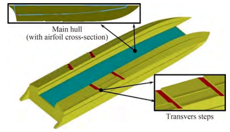 Figure 1 View of the vessel under investigationTable 1 Principal characteristics of the vessel
Particulars Size Length between perpendiculars LPP (mm) 1 000 Breadth B (mm) 300 Demihull breadth BD (mm) 80 Inner deadrise angle βInner (°) 90 Outer deadrise angle βOuter (°) 14.5 Displacement Δ (kg) 5.3, 4.6, 4 LCG from the transom (30%, 40%, 35%) LPP Draft T (mm) 48, 51, 46 Static trim (°) 1.26, −1.3, 0.6 Three displacements of 5.3, 4.6, and 4 kg with the centers of gravity of 30%, 40%, and 35% of the stern length of the vessel, respectively, were considered for the vessel. The distance of the center of gravity from the stern of the vessel was chosen such that it was located at the site of the transverse stairs and between the two steps. The resistance force for the displacement of 5.3 kg was calculated through the experimental method. Then, by using the numerical method, the dynamic components and vessel behavior in all weighted states were investigated and analyzed.
3 Problem definition
Experimental study data were applied to validate the numerical results. Experiments were carried out in the National Iranian Marine Laboratory (member of the International Towing Tank Conference (ITTC)). The main characteristics of the towing tank are presented in Table 2. The tests were performed by following ITTC recommendations (ITTC 2002). The vessel model for testing was installed under the carriage, which consisted of two dynamometers capable of measuring longitudinal, transverse, and torque forces. Figure 2 shows a view of the equipment mounted on the vessel tested at the Froude number of 1.55. This model was tested with the displacement of 5.3 kg and LCG of 30% of the length waterline from the stern at the Froude numbers of 0.49–2.91. In the experiments, the horizontal component of the resistant force of vessel forward motion was measured at a constant speed by using a dynamometer (in kilograms force) (Table 3). In all the tests, the heaving and pitching movements of the vessel were free, and the tests were carried out with three degrees of freedom (heaving, pitching, and forward speeding). During the experiments, the resistance force increased with the increase in the Froude number. At the Froude number of 2.91, porpoising longitudinal instability occurred because of the combination of heaving and pitching movements.
Table 2 NIMALA towing tank specificationsParticulars Size Length of the canal (m) 400 Width of the canal (m) 6 Depth of the canal (m) 4 Maximum velocity of the carrier (m/s) 18 Density water (kg/m3) 1 002 Kinematic viscosity water (m2/s) 9.67 × 10⁷ Water temperature (℃) 21 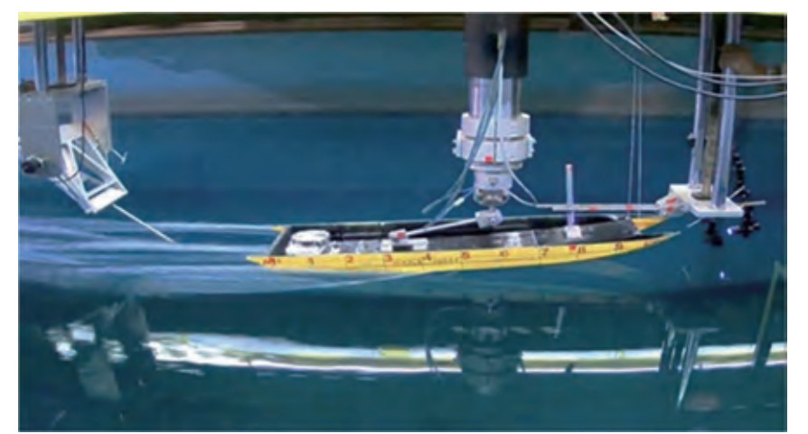 Figure 2 View of the vessel under investigationTable 3 Results of the tests conducted on the vessel model
Length Froude number Total resistance (N) 0.49 7.26 0.98 9.61 1.55 12.75 1.94 - 2.43 - 2.91 Unstable Uncertainties in the experimental analysis were studied in accordance with the guidelines provided by the ITTC (2014a). Accordingly, in the uncertainty analysis of measured resistance, the following variables were considered:
• Hull geometry
• Calibration of measuring equipment (dynamometer)
• Water temperature
• Towing speed
• Measured results
The geometric model studied in this experiment was made of fiberglass (Figure 3). The built vessel model was compared with a model designed by using software in accordance with ITTC recommendations. ITTC criteria state that the model hull tolerances for breadth and depth should be within ±1 mm, and the tolerances for model length should be within 0.05%LPP or 1 mm, whichever is larger. Transverse sections were taken at certain longitudinal distances from the hull to measure the model error. Then, the size of the model was measured at different locations. The measurements showed errors of less than 1 mm, indicating the accuracy of the constructed model. Moreover, the equipment was calibrated in accordance with standards, and the accuracy of its performance has been proven many times in various experiments. The density and viscosity of water were determined in accordance with ITTC standards on the basis of water temperature. The experiments were repeated five times at each speed to calculate the resistance force. The uncertainty analysis results of total resistance at different length Froude numbers are presented in Table 4. The results showed that the uncertainty of resistance force was less than 1% at different length Froude numbers.
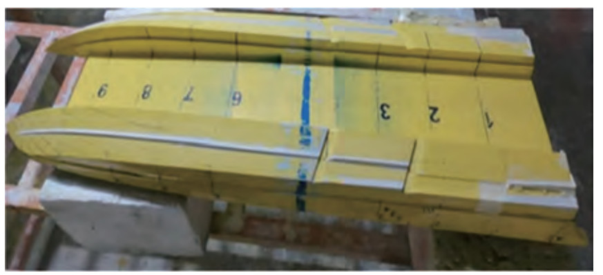 Figure 3 View of the vessel under investigationTable 4 Summary of the uncertainty analysis of total resistance
Length Froude number Uc' (RT) (%) 0.49 0.98 0.98 0.84 1.55 0.79 4 Numerical study
In this study, Siemens PLM Star CCM+ 2021.2 software was applied to analyze the aerodynamics and hydrodynamics of vessel behavior. This software uses the finite volume method to solve governing equations. Simulations were performed at different displacements and speeds on the basis of the RANS solver. Moreover, the numerical results were compared and validated with experimental data. Then, with the development of the numerical study, the effect of water and air fluids was evaluated in terms of parameters, such as resistance, trim, sinkage, and lift force.
4.1 Governing equations
In this study, water and air fluids were considered Newtonian and incompressible. Accordingly, the continuity and momentum equations governing flow were defined as follows:
$$ \nabla \cdot \boldsymbol{V}=0 $$ (1) $$ \rho\left(\frac{\partial V}{\partial t}+\nabla\right)=\nabla \boldsymbol{p}+\nabla \cdot\left[\mu\left(\nabla \cdot \boldsymbol{V}+(\nabla \cdot \boldsymbol{V})^{\mathrm{T}}\right)\right]-g K $$ (2) In these equations, V is the velocity vector, ρ is the fluid density, and μ is the dynamic viscosity coefficient. A suitable turbulence model should be used to model flow. Accordingly, in the present study, the SST k-ω turbulence model was implemented with the following equations (Bi et al. 2020):
$$ v_T=\frac{a_1 k}{\max \left(a_1 \omega ; \mathrm{SF}_2\right)} $$ (3) $$ \frac{\mathrm{D} \rho k}{\mathrm{D} t}=\frac{\partial}{\partial x_j}\left[\left(\mu+\sigma_k \mu_t \frac{\partial k}{\partial x_j}\right)\right]+\tau_{i j} \frac{\partial u_i}{\partial x_j}-\beta^* \rho \omega k $$ (4) $$ \begin{gathered} \frac{\mathrm{D} \rho \omega}{\mathrm{D} t}=\frac{\partial}{\partial x_j}\left[\left(\mu+\sigma_\omega \mu_t \frac{\partial \omega}{\partial x_j}\right)\right]+\frac{\gamma}{v_t} \tau_{i j} \frac{\partial u_i}{\partial x_j}-\beta \rho \omega^2\\ +2\left(1-F_1\right) \rho \sigma_{\omega 2} \frac{1}{\omega} \frac{\partial k}{\partial x_j} \frac{\partial \omega}{\partial x_j} \end{gathered} $$ (5) $$ F_2=\tanh \left(\arg _2^2\right) $$ (6) $$ \arg _2=\max \left(2 \frac{\sqrt{k}}{0.09 \omega y^{\prime}} ; \frac{500 v}{y^2 \omega}\right) $$ (7) In the mentioned equations, the constant coefficients of σω, σk, and β are the result of combining the constant coefficients of the two models of k-ɛ and k-ω turbulence. The constant coefficients of ϕ1 and ϕ2 were determined in accordance with Table 5.
$$ \varphi=\varphi_1 F_1+\varphi_2\left(1-F_1\right) $$ (8) $$ F_1=\tanh \left(\arg _4^1\right) $$ (9) $$ \arg ^1=\min \left(\max \left(\frac{\sqrt{k}}{0.09 w y^{\prime}} ; \frac{500 v}{y^2 w}\right) ; \frac{4 \rho \sigma_{\omega 2} k}{\mathrm{CD}_{k w} y^2}\right) $$ (10) $$ \mathrm{CD}_{k \omega}=\max \left(2 \rho \sigma_{\omega 2} \frac{1}{\omega} \frac{\partial k}{\partial x_j} \frac{\partial \omega}{\partial x_j} ; 10^{-20}\right) $$ (11) Table 5 Constant coefficients in turbulence model equationsϕ2 ϕ1 a1 = 0.31 a1=0.31 σk2 = 1 σk1 = 0.85 σω2 = 0.856 σω1=0.5 β2 = 0.082 8 β1=0.075 β* = 0.09 β*=0.09 k = 0.41 k = 0.41 $ \gamma_2=\frac{\beta_2}{\beta^*}-\frac{\sigma_{\omega 2} k^2}{\sqrt{\beta^*}} $ $ \gamma_1=\frac{\beta_1}{\beta^*}-\frac{\sigma_{\omega 1} k^2}{\sqrt{\beta^*}}$ The volume of fluid (VOF) method was applied for free surface modeling. This method describes the geometry surface between the two phases in the form of the following equation:
$$ \frac{\partial \alpha}{\partial t}+\nabla \cdot(\boldsymbol{V} \alpha)=0 $$ (12) α is the volume fraction that is considered as 0 and 1 for water and air fluids, respectively. The density and viscosity characteristics of the two fluids were calculated on the basis of the α value in accordance with two relationships in the form of the following equations:
$$ \rho(\alpha)=\alpha \rho_a+(1-\alpha) \rho_w $$ (13) $$ \mu(\alpha)=\alpha \mu_a+(1-\alpha) \mu_w $$ (14) 4.2 Computational domain and time step
The computational domain size was determined to comply with the minimum ITTC criteria (ITTC 2014b) (Figure 4). Accordingly, the computational domain was extended 2.5L to the front of the bow, which was considered an inlet boundary. The distance from the stern to the outlet boundary was determined to be 12L to ensure the absence of reverse flow and to model the wake created behind the vessel well. The distances of the free surface from the top and bottom of the domain were 2 and 3 times the vessel length, respectively. In addition, the distance from the sidewall of the computational domain to the vessel was 3L to ensure that the lateral boundary did not affect vessel behavior. The time step used in the simulations as a function of vessel speed and wetted length was determined in accordance with the ITTC (2014c) and is given in Equation (15).
$$ \Delta t=0.01 \sim 0.005 \frac{l}{V} $$ (15) 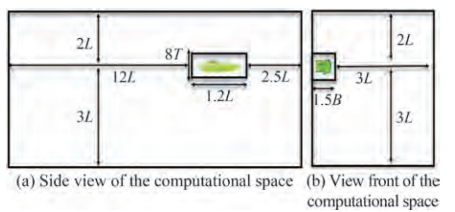 Figure 4 The main dimensions of the computational domain
In this equation, V and l represent the speed and the wetted keel length, respectively. Furthermore, the time step is a function of the grid density to keep the CFL number constant (greater than 1).
4.3 Boundary conditions
The specified boundary conditions are shown in Figure 5. The inlet, side, bottom, and top boundaries were taken as the velocity inlet, and the outlet boundary was considered as the pressure outlet. Simulation was performed symmetrically in accordance with vessel hull symmetry and fluid flow. The hull of the vessel was considered rigid (no-slip wall). As a result, the body surface was considered under no-slip wall boundary conditions.
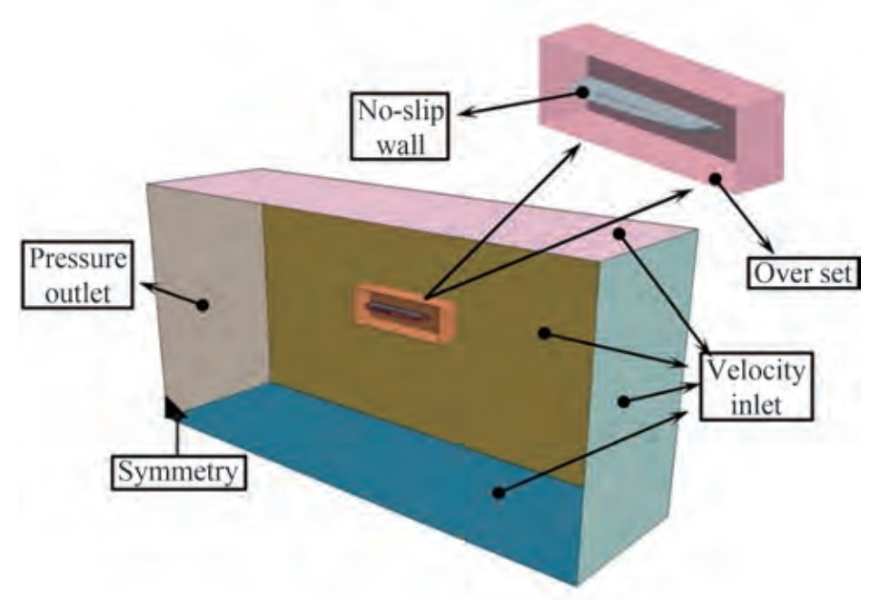 Figure 5 Boundary conditions of the computational domain
4.4 Grid generation
Figure 6 shows the meshing of the different parts of the computational domain. Carrica et al. (2007) demonstrated that in the simulation of vessel movements, applying dynamic mesh increases the accuracy of computations. Furthermore, Begovic et al. (2015) showed that employing unstructured meshing in dynamic mesh (overset region) and structured meshing in other parts of the computational domain (background region) reduces mesh number and computational time. Accordingly, the present study used a dynamic meshing (overset) technique with unstructured hexagonal meshing around the vessel. Given the VOF model and significant waves created behind the vessel, meshing was considered fine on the boundary between the two phases.
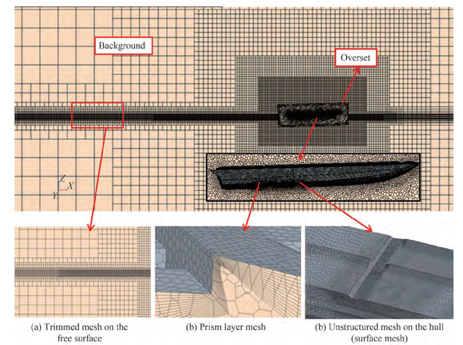 Figure 6 Computational domain meshing
As the hull speed increases, air diffusion under the hull increases because of high trim values. This phenomenon causes an error in the numerical ventilation problem. Numerical ventilation is a well-known problem encountered in the modeling of planing hulls by using the VOF model. This problem may lead to an unwanted drag reduction of up to 30% (Avci and Barlas 2018). Gray-Stephens et al. (2019) and Samuel et al. (2021) investigated different methods for solving numerical ventilation errors. In this study, the two methods of the modified HRIC scheme and mesh refinement were used simultaneously in accordance with the research conducted by Gray-Stephens et al. (2019) to prevent numerical ventilation error. In this research, two methods of mesh refinement were used. Refinement 1 focused around the ship's bow as shown in Figure 7(a), and refinement 2 focused around the ship as illustrated in Figure 7(b).
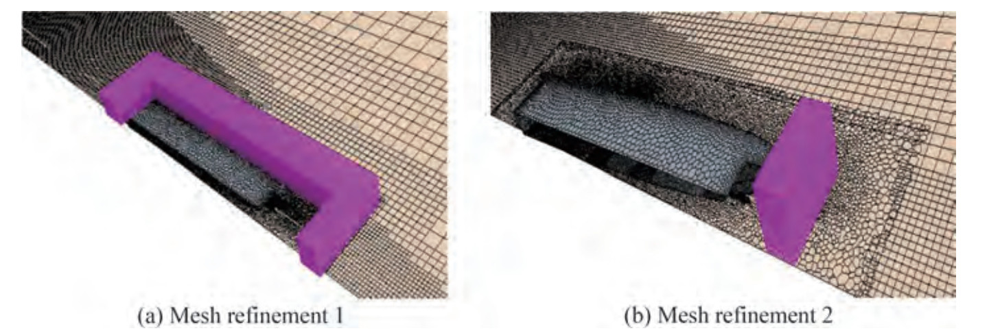 Figure 7 Visualization of mesh refinements 1 and 2
Prismatic layer mesh was used to simulate the boundary layer near the wall (vessel body). The value of the prismatic layer meshing components was determined on the basis of the appropriate y+ value for the proper simulation of turbulence. The ITTC recommendations (ITTC 2014d) state that when the wall function is implemented, the y+ value can be between 30 and 300. The value of y+ was less than 100 at all different speeds and weight modes. The y+ value at each point of the craft at the Froude number of 1.55 and displacement of 5.3 kg is shown in Figure 8.
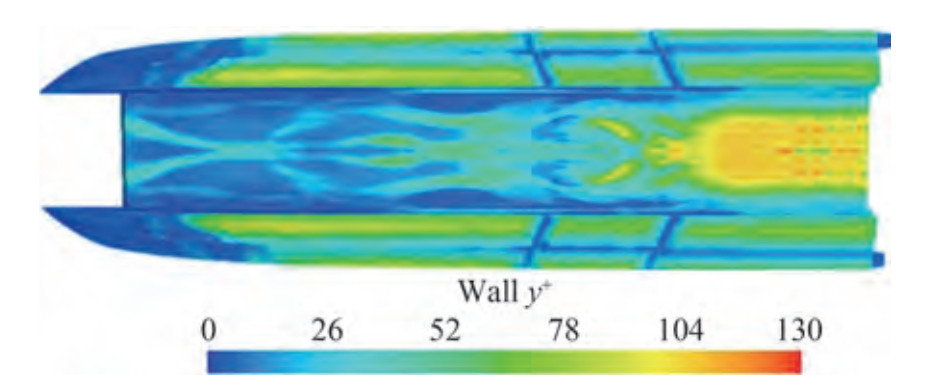 Figure 8 Values of y+ at different points of the craft at the Froude number of 1.55 and displacement of 5.3 kg
4.5 Mesh independency study
This simulation investigated the effect of mesh size at four levels of meshing from coarse to fine. Studies were conducted at the displacement of 5.3 kg and the Froude number of 1.55. Table 6 compares the results of the numerical method with the experimental results obtained in different meshing modes. The results showed that with the increase in the number of meshes, the stability of problemsolving first increased. However, from the third case onward, increasing the number of meshes had no significant effect on the results, and the solution became independent of the number of meshing's. Accordingly, the third mode of meshing, namely, the base of the meshing, was considered to have sufficient accuracy in problem-solving and to reduce computational time.
Table 6 Calculated resistance in different meshingResults Base size Number of mesh RT (N) Error (%) Overset Background Experimental - - - 12.75 - Numerical 0.35LPP 0.43LPP 34 × 104 11.277 11.85 0.25LPP 0.31LPP 72 × 104 11.964 7 0.18LPP 0.22LPP 172 × 104 12.45 3.12 0.12LPP 0.15LPP 380 × 104 12.55 2.34 The grid convergence method was used to evaluate mesh sensitivity, as suggested by Celik et al. (2008). The method used to estimate discretization error was based on the extrapolation method reported by Richardson (1911). This method determines the uncertainty of numerical results by using the results of three different meshings. In the first step, the mesh dimensions were calculated by using Equation (16).
$$ {h_i} = {\left[ {\frac{1}{N}\sum\limits_{i = 1}^n {{V_i}} } \right]^{\frac{1}{3}}} $$ (16) The dimensions of the mesh at each stage should be such that Equation (17) is established as
$$ \frac{h_i}{h_{i+1}}>1.3 $$ (17) Then, the average of the apparent order of the method takes the following form:
$$ p_{\mathrm{avg}}=\frac{1}{\ln \left(r_{21}\right)}|\ln | \varepsilon_{32} / \varepsilon_{21}|+q(p)| $$ (18) $$ q(p)=\ln \left(\frac{r_{21}^p-s}{r_{32}^p-s}\right) $$ (19) In Equation (18), the parameters r21 and r32 indicate the grid refinement factors that are determined by $ \sqrt 2 $. Moreover, ε32 = ϕ3 – ϕ2, ε21 = ϕ2 – ϕ1, and ϕk denotes the solution on the kth grid. φ is the key variable in problem-solving. In this simulation, this variable was the resistance value. The relative extrapolation error value was determined in accordance with Equations (19) to (23).
$$ \phi_{\mathrm{txt}}^{32}=\frac{\left(r_{21}^{p_{\mathrm{avg}}} \phi_1-\phi_2\right)}{\left(r_{21}^p-1\right)} $$ (20) $$ e_a^{32}=\left|\frac{\phi_2-\phi_3}{\phi_2}\right| $$ (21) $$ e_{\mathrm{ext}}^{32}=\left|\frac{\phi_{\mathrm{ext}}^{23}-\phi_3}{\phi_{\mathrm{ext}}^{23}}\right| $$ (22) $$ \mathrm{GCI}_{\mathrm{fine}}^{32}=\frac{1.25 e_a^{32}}{r_{32}^{p_{\mathrm{avg}}}-1} $$ (23) These parameters were calculated for the considered hydrodynamics resistance and are shown in Table 7.
Table 7 Discretization error for hydrodynamics resistance based on the grid convergence methodItems Total resistance r21 $ \sqrt 2 $ r23 $ \sqrt 2 $ ϕ1 12.55 ϕ2 12.45 ϕ3 11.964 pavg 5.304 ϕtxt32 12.582 ea32 0.797 eext32 0.259 GCIfine32 0.325 4.6 Comparison of numerical and experimental results
The numerical simulation results for the displacement of 5.3 kg were compared with similar experimental data for validation (Table 8). A comparison of the resistance force results showed that the maximum error at all studied speeds did not exceed 4.36%. Therefore, numerical simulation has good accuracy and correctly predicts the trend of resistance variations with the increase in the Froude number.
Table 8 Comparison of experimental and numerical results at the displacement of 5.3 kgDisplacement (kg) Froude number Resistance force (N) Error (%) Experimental Numerical 5.3 0.49 7.26 7.07 3.03 0.97 9.61 9.22 4.36 1.55 12.75 12.45 3.12 1.94 - 14.22 - 2.43 - 15.89 - 2.91 Unstable Unstable - 5 Results and discussion
An analysis of the results of dynamic parameters, such as resistance force, lift, trim, and sinkage, is provided in this section. The results for the abovementioned displacements different Froude numbers are presented. Moreover, the pressure distribution at the bottom of the vessel, wave profiles, and the wetted surface in different modes are shown and investigated. The studied vessel used the lift force obtained from water and air fluids to withstand the weight force. Accordingly, the contributions of water and air fluids to vessel behavior in the simulations were calculated and investigated separately. Accordingly, the contribution of water and air fluids was studied in all simulations.
5.1 Resistance force
The resistance force caused by the fluid against a moving craft, especially at high speeds, is one of the important and effective parameters for increasing the velocity of highspeed vessels. The power required to reach high speeds increases with the increase in resistance force. Therefore, investigating the dynamic behavior of each craft by changing the speed is necessary. The resistance force at different Froude numbers and the displacements of 5.3, 4.6, and 4 kg are shown in Figure 9. The results showed that in all displacement modes, the resistance force increased with the increment in the Froude number. The vessel was stable at the displacement of 5.3 kg up to the Froude number of 2.43 and then experienced longitudinal instability. Moreover, the vessel was stable at the displacement of 4.6 kg up to the Froude number of 2.9. The vessel was stable at the displacement of 4 kg up to the Froude number of 1.95 and suffered from instability at high Froude numbers. The contributions of water and air fluids to frictional resistance at different Froude numbers and the mentioned displacement are presented in Figure 10. The results illustrated that the frictional resistance of the air increased with an increase in the Froude number and the reduction in the wetted surface of the hull. However, given that the density and viscosity of water are considerably higher than those of air, the frictional resistance of water was higher than that of air at all Froude numbers. In general, the contribution of air to the creation of frictional resistance was less than 15%. Figure 11 displays the contribution of water and air fluids to pressure resistance. Accordingly, the pressure resistance caused by the two water and air fluids decreased and increased with the increase in Froude number and vessel position in the planing motion mode, respectively. Therefore, at the mentioned displacements, air pressure resistance in the planing mode increased by 55%, 40%, and 60% relative to those in the displacement mode.
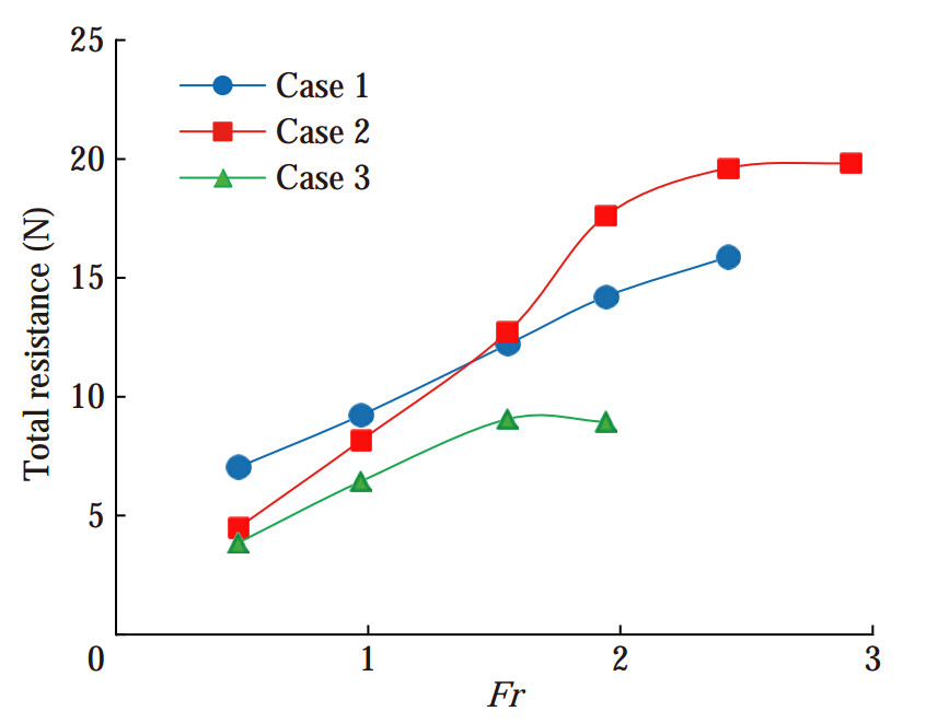 Figure 9 Resistance of the force at different Froude numbers
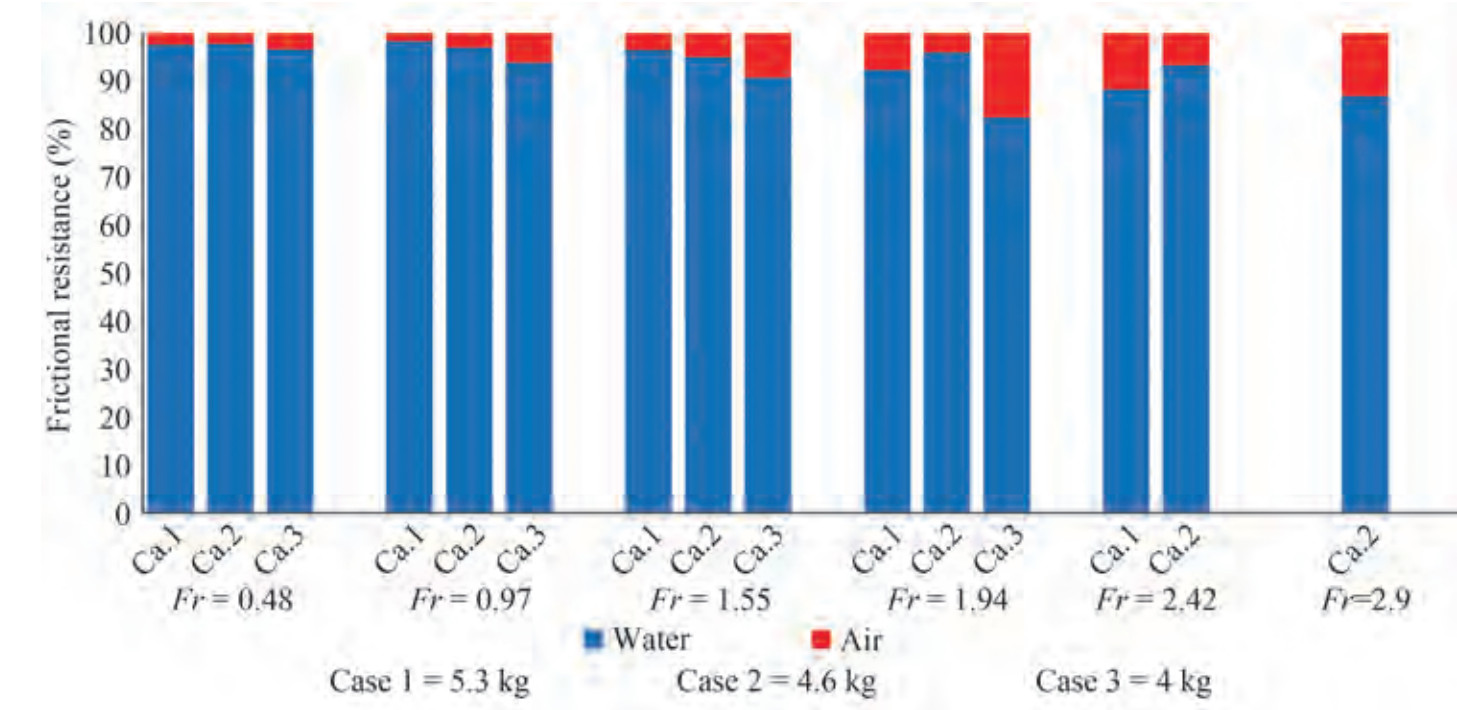 Figure 10 Contribution of water and air fluids to frictional resistance at the displacements of 5.3, 4.6, and 4 kg
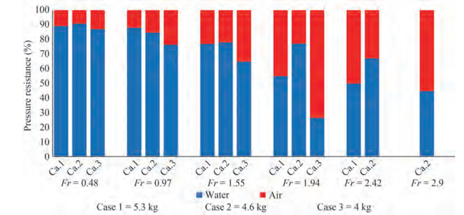 Figure 11 Contribution of water and air fluids to pressure resistance at the displacements of 5.3, 4.6, and 4 kg
5.2 Trim and sinkage
This work investigated the dynamic behavior of a craft at two degrees of freedom, namely, heaving and pitching. The trim (tumbling around the longitudinal axis) and sinkage (linear motion in the vertical axis direction) diagrams at different Froude numbers are shown in Figure 12 and Figure 13, respectively. At the displacements of 5.3 and 4 kg, the vessel trim decreased until the Froude number of 1.5 and then increased. At the displacement of 4.6 kg, the vessel trim increased until it reached the planing mode (Fr = 1), then decreased until the Froude number of 1.5, and subsequently increased. At the displacements of 5.3 and 4 kg, vessel sinkage increased up to the Froude number of 1.95. Its slope then decreased, and it further declined. Moreover, at the displacements of 5.3 and 4 kg, vessel sinkage increased with the increase in Froude number and the change in vessel motion from displacement to planing.
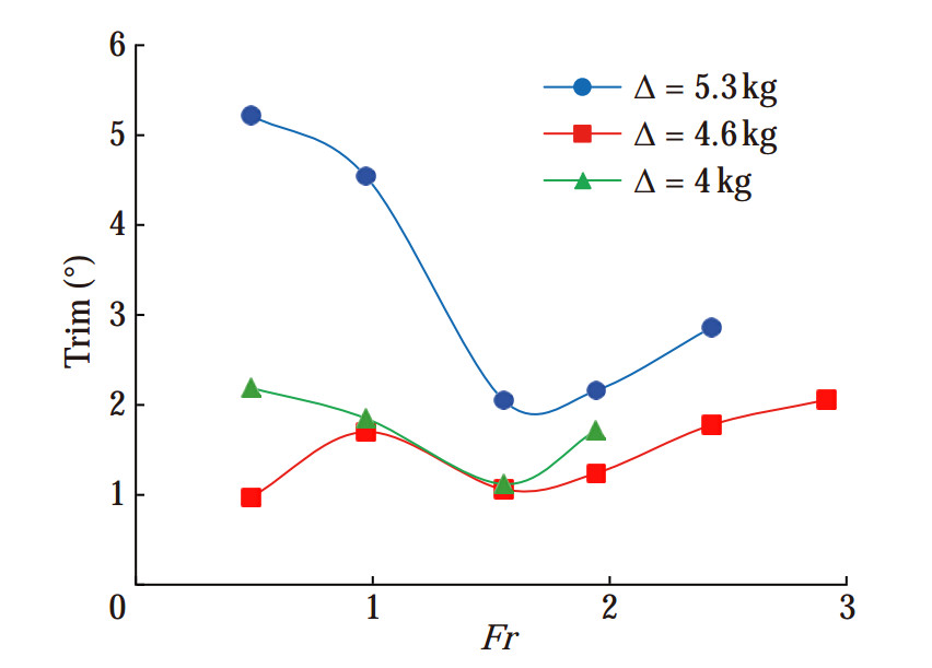 Figure 12 Vessel trim at different Froude numbers and the displacements of 5.3, 4.6, and 4 kg
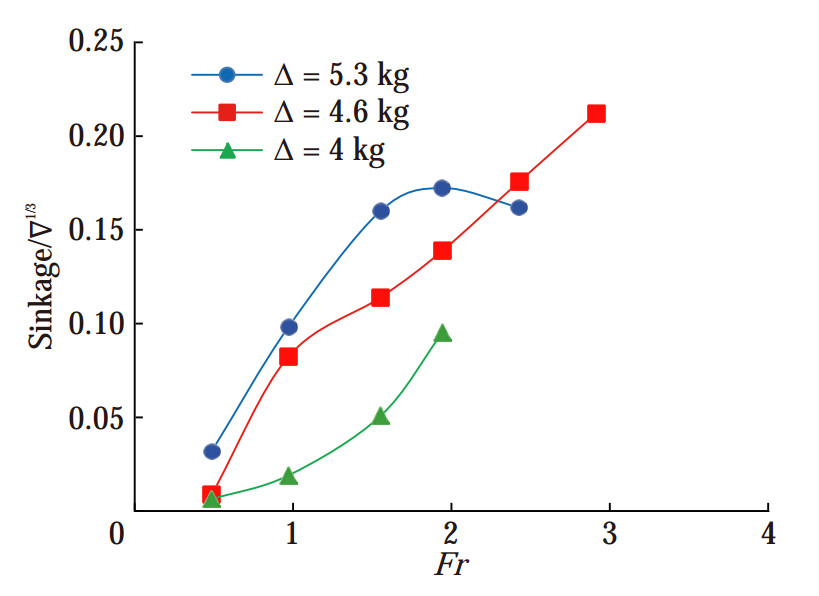 Figure 13 Vessel sinkage at different Froude numbers and the displacements of 5.3, 4.6, and 4 kg
5.3 Wetted surface
The wetted area is the vessel hull area that has been immersed in water. In ships, especially high-speed planing vessels, the wetted surface is directly related to the overall hydrodynamics drag. The wetted surface changes at different Froude numbers in accordance with vessel behavior. The ratios of the area of the dry and wetted surface to the surface area of the hull are shown in Figure 14. During planing movement, the wetted surface of the vessel at different displacements decreased with the increase in the Froude number and vessel exposure, and the majority of the surface of the hull was exposed to air. At the three displacements of 5.3, 4.6, and 4 kg under these conditions, the wetted surfaces of the vessel reduced in the planing mode relative to those in the displacement mode by 20%, 15%, and 25%, respectively. The wetted surfaces of the vessel in the displacement (Fr = 0.48), semidisplacement (Fr = 0.98), and planing (Fr =1.94) motion modes at different weights are illustrated in Figure 15. The wetted surface of the vessel decreased with the increase in the Froude number of the wetted surface.
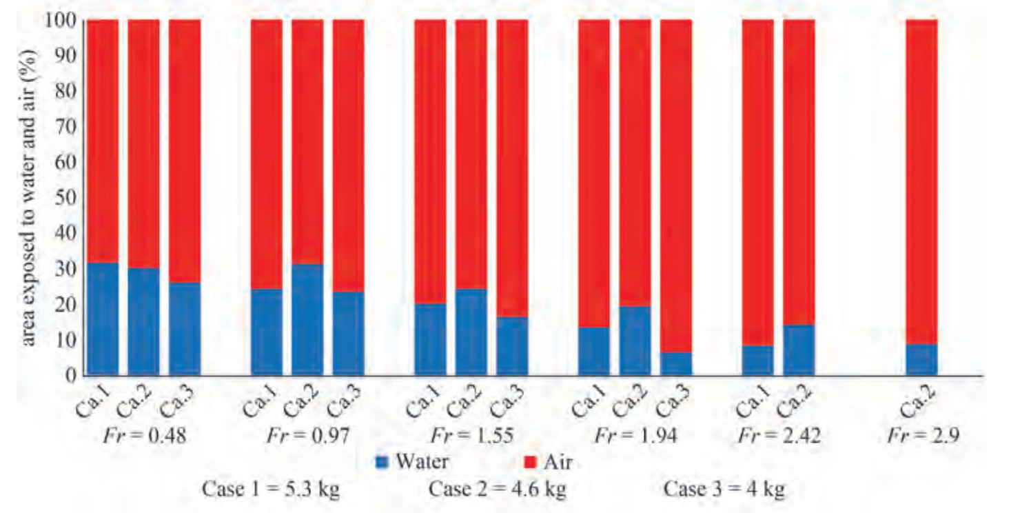 Figure 14 Surface exposed to the flow of water and air fluids at different froude numbers
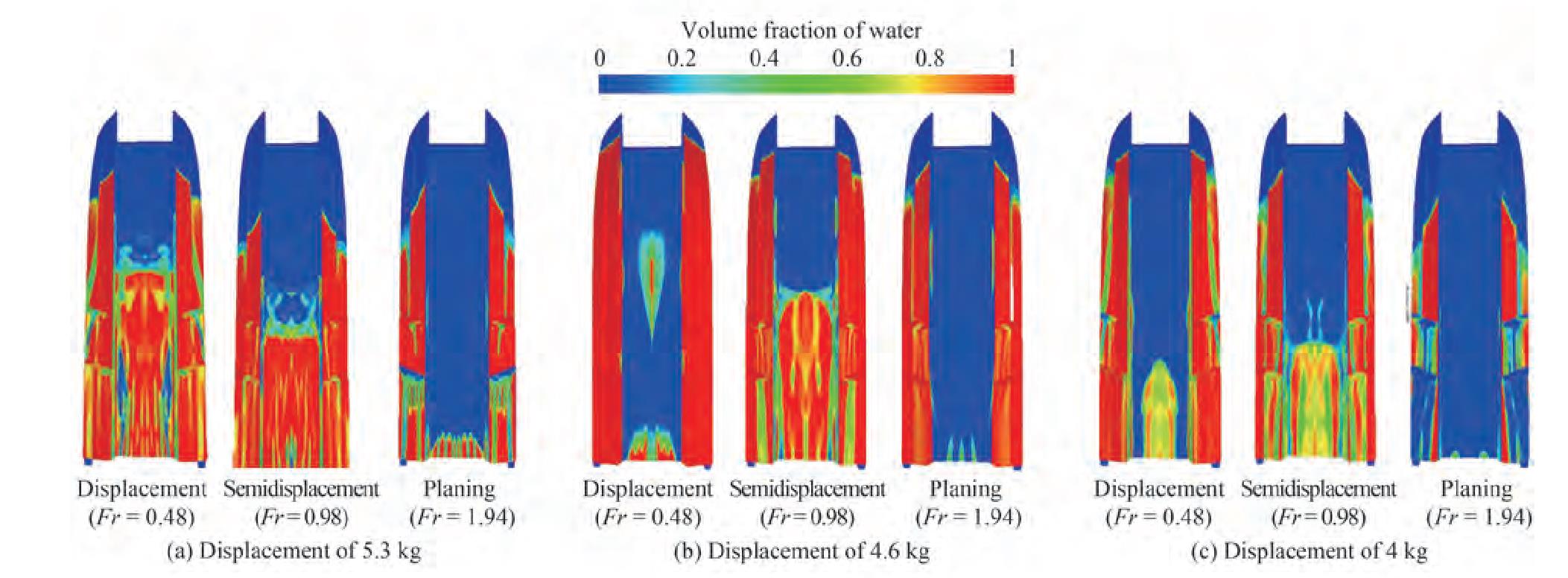 Figure 15 Wetted surface of the vessel bottom in motion modes
5.4 Lift force
In displacement mode, the buoyancy force held almost all vessel weight forces. More than half of the vessel weight force was held in planing mode by the dynamic forces caused by two water and air fluids. The lift forces at the different Froude numbers at the displacements of 5.3, 4.6, and 4 kg are presented in Figure 16. In planing mode, the wetted surface of the vessel decreased with the increase in Froude number and thus increased the lift force contributed by air. The results showed that the contributions of air to the creation of lift force in planing mode were 60%, 50%, and 70% for the mentioned displacements. However, the contribution of air to the creation of lift force in the displacement mode was less than 10%.
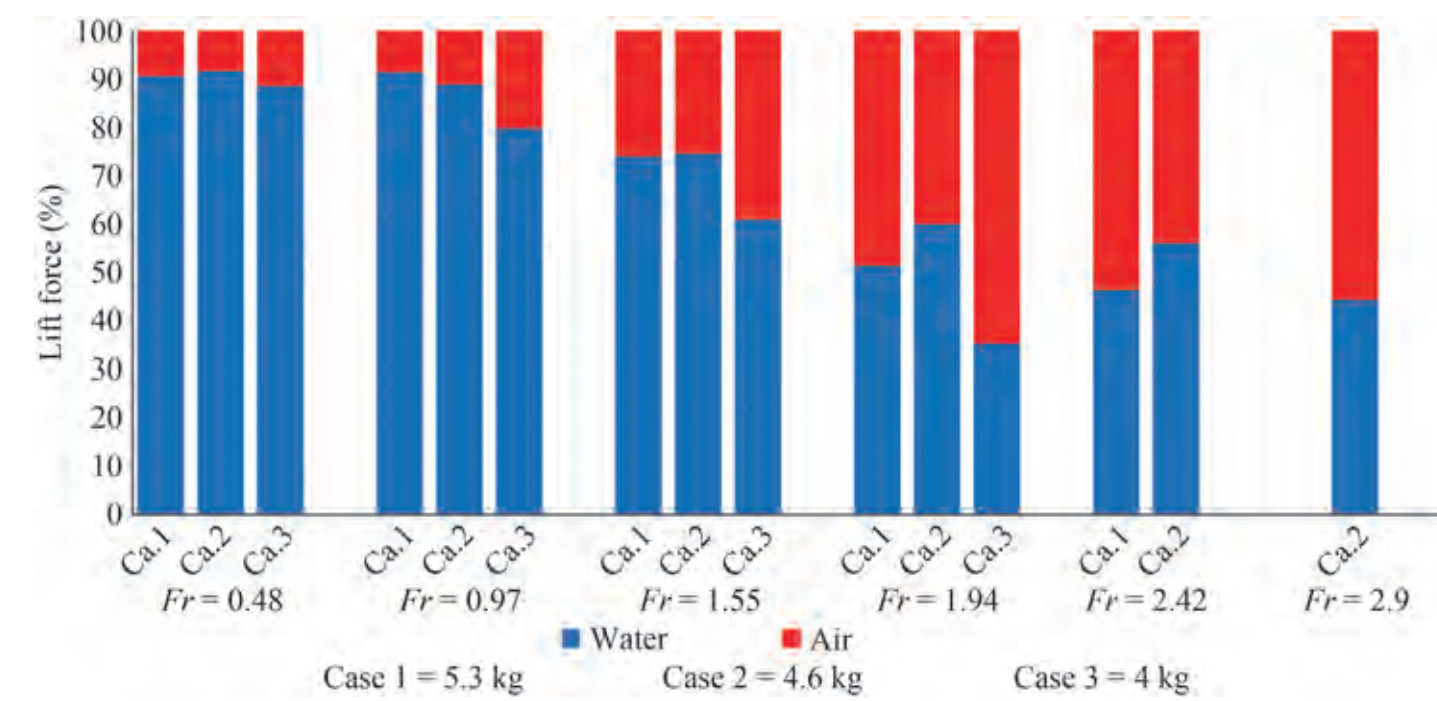 Figure 16 Contribution of water and air fluids to lift force at the displacements of 5.3, 4.6, and 4 kg
5.5 Wake created by the vessel
As a high-speed vessel moves in the water, it builds up a wake behind the vessel hull. The range of the wake created behind a vessel varies at different speeds. Figure 17 shows a schematic of the amplitude and height of the wake created behind the vessel. Figure 18 presents the highest height and amplitude of the wake created behind the vessel at different Froude numbers and displacements. The penetration rate of the vessel stern in water decreased with the reduction in trim. Therefore, due to the continuity of the water fluid, the height of the wake created behind the vessel decreased. Moreover, by increasing the Froude number, the speed of the flow behind the transom caused the wake to occur at a distance far from the stern. Figure 19 shows the wake created behind the vessel at different displacements and in the modes of displacement (Fr = 0.48), semidisplacement (Fr = 0.98), and planing (Fr = 1.94).
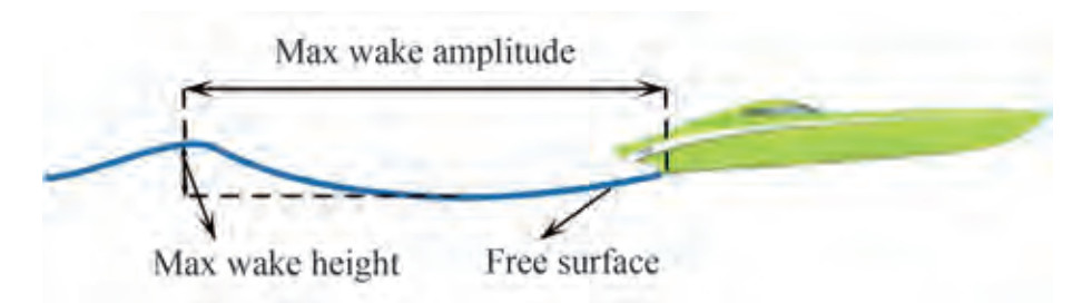 Figure 17 Schematic of the amplitude and height of the wake
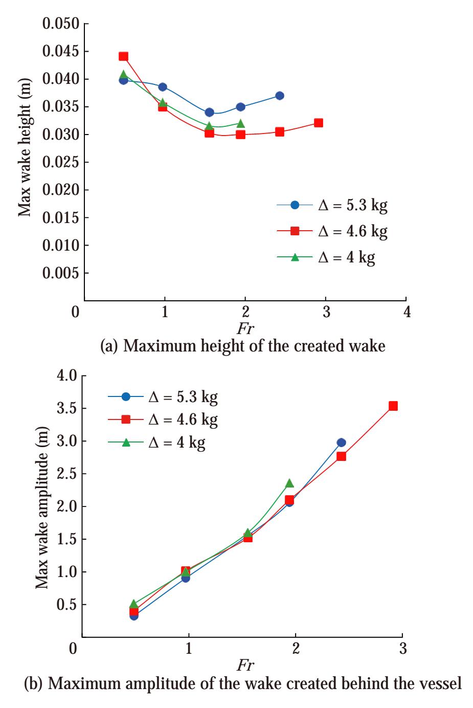 Figure 18 The specification of the wake created behind the vessel
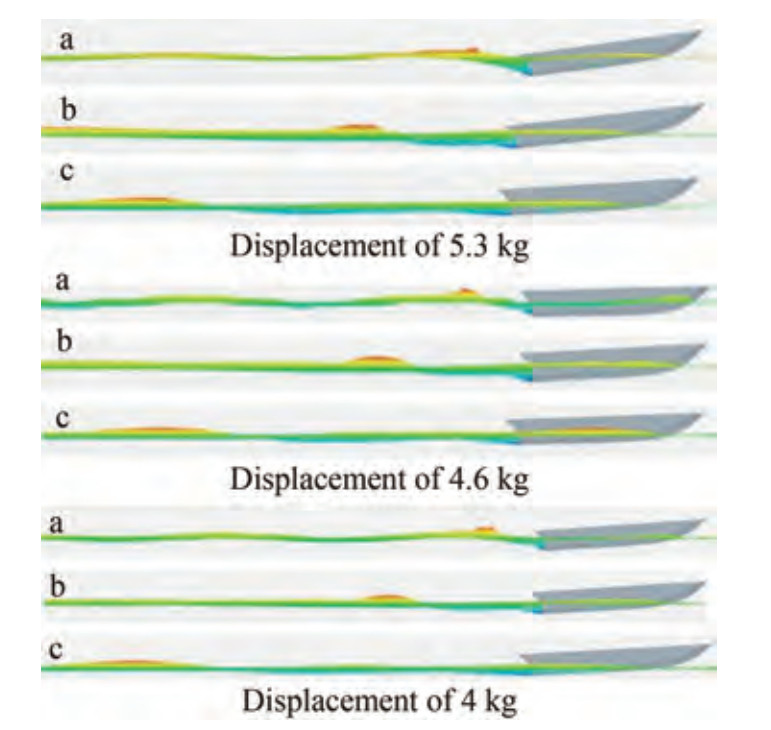 Figure 19 Wake created behind the vessel in motion modes, a: displacement (Fr = 0.48), b: semidisplacement (Fr = 0.98), c: planing (Fr = 1.94)
5.6 Wave pattern around the craft
Figure 20 shows the wave pattern created by the vessel at the displacements of 5.3, 4.6, and 4 kg in the motion modes of displacement (Fr = 0.48), semidisplacement (Fr = 0.98), and planing (Fr = 1.94). The length of the wake created behind the vessel increased with the rise in the Froude number. Longer waves dissipated later than shorter waves. Accordingly, the wave pattern created behind the vessel lengthened and narrower. As a result, it can be said that "narrowed with the increase in speed. Therefore, the length and angle of the wave pattern created by increasing the velocity have direct and inverse relationships, respectively.
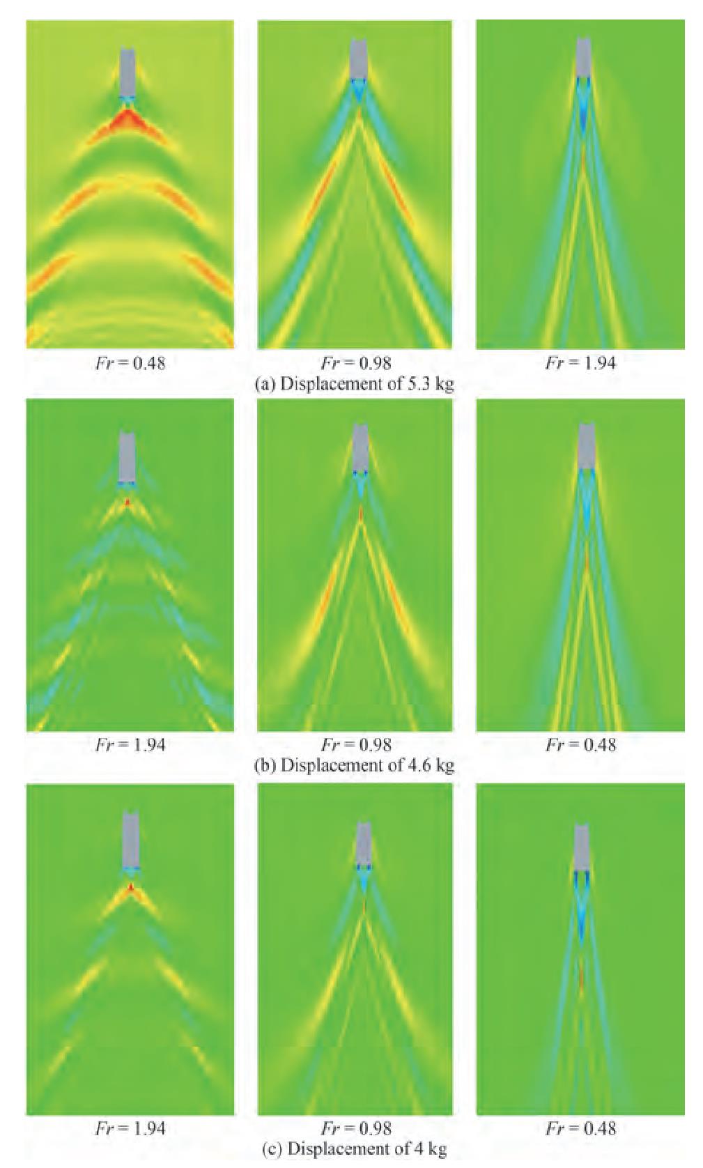 Figure 20 Wave pattern created around the vessel at the displacements of 5.3, 4.6, and 4 kg
5.7 Pressure distribution
The pressure distribution on the vessel bottom was analyzed in two different longitudinal plates. The placement of these plates on the vessel bottom is shown in Figure 21. These two plates were considered at distances of 0 and 0.155 m from the vessel's centerline.
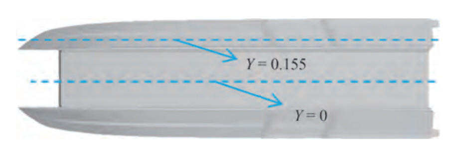 Figure 21 Longitudinal sections on the bottom of the vessel
The contour and diagram of pressure changes in the two mentioned plates at the displacement of 5.3 kg in the motion modes of displacement (Fr = 0.48), semidisplacement (Fr = 0.98), and planing (Fr = 1.94) are shown in Figure 22 and 23. The stagnation line in the main hull approached the stern with the increase in the Froude number and the change in the vessel motion mode from displacement to planing (Figure 22(b)). Moreover, the pressure increased on the demihull's bow, thus affecting the hull flow (Figure 22(a)). Furthermore, the steps of the bottom of the vessel separated the flow and created a stagnation line on their back that increased the pressure.
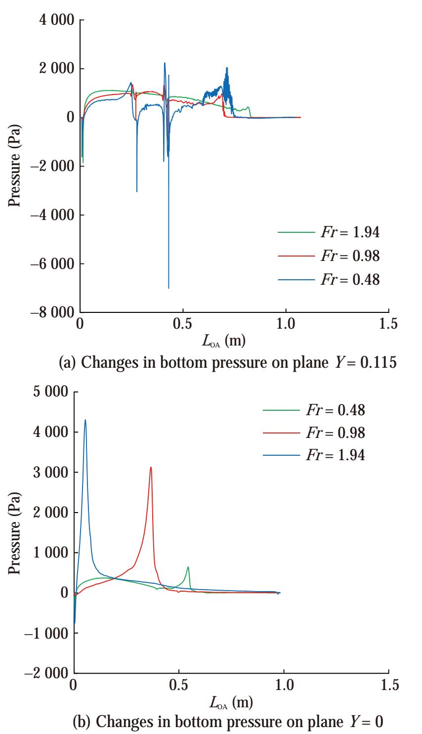 Figure 22 Changes in bottom pressure on plane Y = 0.115 and plane Y = 0 in the modes of motion of displacement, semidisplacement, and planing
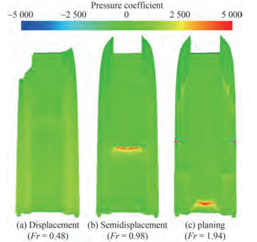 Figure 23 Pressure contour on the bottom of the craft in three modes
5.8 Porpoising longitudinal instability
The displacement of the center of pressure around the center of gravity creates longitudinal instability in a vessel. This instability is called porpoising instability. Porpoising causes intermittent dynamic instability during heaving and pitching movements. The oscillation range of the motion of pitching and heaving for different displacements at the Froude numbers of 2.4 and 2.9 are presented in Table 9. At the displacement of 5.3 kg, the vessel was stable at the Froude number of 2.4 and became unstable with the increase in Froude number. Moreover, the craft was entirely stable at the displacement of 4.6 kg and did not suffer from porpoising instability. At the displacement of 4 kg, vessel instability began at the Froude number of 2.4 and intensified with the increase in the Froude number of the oscillations created during pitching and heaving.
Table 9 Average oscillation of pitching and heaving movementsDisplacement (kg) LCG Froude number Pitch oscillation average (°) Heave oscillation average (mm) 5.3 30%LWL 2.4 Stability Stability 2.9 0.5 15 4.6 40%LWL 2.4 Stability Stability 2.9 Stability Stability 4 35%LWL 2.4 0.3 10 2.9 1.2 13 The pressure contours of the vessel bottom at the Froude numbers of 1.94 (stable conditions) and 2.9 (unstable conditions) for the mentioned displacements are presented and compared in Figure 24. At the Froude number of 1.94, the center of gravity was located at the displacements of 5.3 and 4 kg away from the maximum pressure zones. The stagnation line moved backward when the speed and trim were increased such that the area under maximum pressure surrounded the center of gravity. Under these conditions, the center of pressure moved around the center of gravity, resulting in the creation of forces and dynamic moments, ultimately causing the Porpoising instability. At the displacement of 4.6 kg, the vessel was stable at both of the mentioned Froude numbers. In this case, the movement of the center of pressure was not around the center of gravity, and instability did not occur in the vessel. As a result, at the displacement of 4.6 kg, the vessel performed well in terms of longitudinal stability.
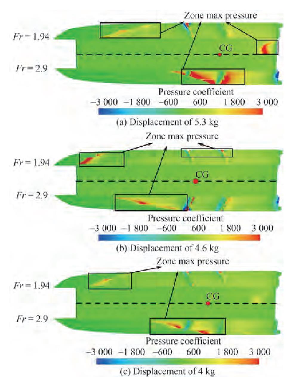 Figure 24 Vessel pressure contour in the steady state (Fr = 1.94) and the unstable state (Fr = 2.9)
6 Conclusions
This paper presents an experimental and numerical investigation of the behavior of a high-speed catamaran planing at the displacements of 5.3, 4.6, and 4 kg. The vessel had two demihulls and a main hull with a foil cross-section that produced lift force hydrodynamics and aerodynamics, respectively. Therefore, evaluating the effect of water and air fluids on the dynamic components of the vessel was necessary. In the experimental study, the resistance force of a catamaran planing at the displacement of 5.3 kg was evaluated by considering the effect of water and air fluids. In numerical studies, the results of numerical simulations were first validated with experimental data. Therefore, for evaluation with increased accuracy, vessel performance was analyzed at the three displacements of 5.3, 4.6, and 4 kg over the Froude number range of 0.49 to 2.9. The most significant results are as follows:
1) At all displacements, the frictional resistance of the air in the displacement motion mode was low. However, in the planing motion mode, frictional resistance reached approximately 15%.
2) In the planing mode, air pressure resistance was approximately equal to water pressure resistance and increased by 55%, 40%, and 60% at the displacements of 5.3, 4.6, and 4 kg, respectively.
3) The wetted surface of the vessel decreased with the increase in Froude number and the change in the mode of motion from displacement to planing. Therefore, compared with that in the displacement mode at the displacements of 5.3, 4.6, and 4 kg, the wetted surface of the craft in the planing mode decreased by 20%, 15%, and 25%, respectively.
4) When the vessel was in the planing mode, increasing the speed increased the air effectiveness of the lift force. In the planing mode, the contribution of air to the creation of lift force at the displacements of 5.3, 4.6, and 4 kg were 60%, 50%, and 70%, respectively.
5) The amplitude and height of the wake were directly related to the speed and trim of the vessel, respectively. Under these conditions, the speed of water increased due to the creation of a water jet behind the vessel, causing the wake to become concentrated in one direction and along the vessel centerline. As the vessel speed increased, the wake created behind the vessel elongated and narrowed.
6) The area under maximum pressure changed along the vessel and approached the center of gravity as the velocity increased and the trim changed. In some cases, by increasing the speed beyond a determined value, the movement of the pressure center around the gravity center caused porpoising longitudinal instability.
The effect of the shape and position of transverse steps on dynamic components and porpoising instability will be considered in future work. Moreover, given that the main hull of this vessel is in the form of a foil, future work will examine the effects of foil components on vessel stability.
-
Figure 1 View of the vessel under investigation
Figure 2 View of the vessel under investigation
Figure 3 View of the vessel under investigation
Figure 4 The main dimensions of the computational domain
Figure 5 Boundary conditions of the computational domain
Figure 6 Computational domain meshing
Figure 7 Visualization of mesh refinements 1 and 2
Figure 8 Values of y+ at different points of the craft at the Froude number of 1.55 and displacement of 5.3 kg
Figure 9 Resistance of the force at different Froude numbers
Figure 10 Contribution of water and air fluids to frictional resistance at the displacements of 5.3, 4.6, and 4 kg
Figure 11 Contribution of water and air fluids to pressure resistance at the displacements of 5.3, 4.6, and 4 kg
Figure 12 Vessel trim at different Froude numbers and the displacements of 5.3, 4.6, and 4 kg
Figure 13 Vessel sinkage at different Froude numbers and the displacements of 5.3, 4.6, and 4 kg
Figure 14 Surface exposed to the flow of water and air fluids at different froude numbers
Figure 15 Wetted surface of the vessel bottom in motion modes
Figure 16 Contribution of water and air fluids to lift force at the displacements of 5.3, 4.6, and 4 kg
Figure 17 Schematic of the amplitude and height of the wake
Figure 18 The specification of the wake created behind the vessel
Figure 19 Wake created behind the vessel in motion modes, a: displacement (Fr = 0.48), b: semidisplacement (Fr = 0.98), c: planing (Fr = 1.94)
Figure 20 Wave pattern created around the vessel at the displacements of 5.3, 4.6, and 4 kg
Figure 21 Longitudinal sections on the bottom of the vessel
Figure 22 Changes in bottom pressure on plane Y = 0.115 and plane Y = 0 in the modes of motion of displacement, semidisplacement, and planing
Figure 23 Pressure contour on the bottom of the craft in three modes
Figure 24 Vessel pressure contour in the steady state (Fr = 1.94) and the unstable state (Fr = 2.9)
Table 1 Principal characteristics of the vessel
Particulars Size Length between perpendiculars LPP (mm) 1 000 Breadth B (mm) 300 Demihull breadth BD (mm) 80 Inner deadrise angle βInner (°) 90 Outer deadrise angle βOuter (°) 14.5 Displacement Δ (kg) 5.3, 4.6, 4 LCG from the transom (30%, 40%, 35%) LPP Draft T (mm) 48, 51, 46 Static trim (°) 1.26, −1.3, 0.6 Table 2 NIMALA towing tank specifications
Particulars Size Length of the canal (m) 400 Width of the canal (m) 6 Depth of the canal (m) 4 Maximum velocity of the carrier (m/s) 18 Density water (kg/m3) 1 002 Kinematic viscosity water (m2/s) 9.67 × 10⁷ Water temperature (℃) 21 Table 3 Results of the tests conducted on the vessel model
Length Froude number Total resistance (N) 0.49 7.26 0.98 9.61 1.55 12.75 1.94 - 2.43 - 2.91 Unstable Table 4 Summary of the uncertainty analysis of total resistance
Length Froude number Uc' (RT) (%) 0.49 0.98 0.98 0.84 1.55 0.79 Table 5 Constant coefficients in turbulence model equations
ϕ2 ϕ1 a1 = 0.31 a1=0.31 σk2 = 1 σk1 = 0.85 σω2 = 0.856 σω1=0.5 β2 = 0.082 8 β1=0.075 β* = 0.09 β*=0.09 k = 0.41 k = 0.41 $ \gamma_2=\frac{\beta_2}{\beta^*}-\frac{\sigma_{\omega 2} k^2}{\sqrt{\beta^*}} $ $ \gamma_1=\frac{\beta_1}{\beta^*}-\frac{\sigma_{\omega 1} k^2}{\sqrt{\beta^*}}$ Table 6 Calculated resistance in different meshing
Results Base size Number of mesh RT (N) Error (%) Overset Background Experimental - - - 12.75 - Numerical 0.35LPP 0.43LPP 34 × 104 11.277 11.85 0.25LPP 0.31LPP 72 × 104 11.964 7 0.18LPP 0.22LPP 172 × 104 12.45 3.12 0.12LPP 0.15LPP 380 × 104 12.55 2.34 Table 7 Discretization error for hydrodynamics resistance based on the grid convergence method
Items Total resistance r21 $ \sqrt 2 $ r23 $ \sqrt 2 $ ϕ1 12.55 ϕ2 12.45 ϕ3 11.964 pavg 5.304 ϕtxt32 12.582 ea32 0.797 eext32 0.259 GCIfine32 0.325 Table 8 Comparison of experimental and numerical results at the displacement of 5.3 kg
Displacement (kg) Froude number Resistance force (N) Error (%) Experimental Numerical 5.3 0.49 7.26 7.07 3.03 0.97 9.61 9.22 4.36 1.55 12.75 12.45 3.12 1.94 - 14.22 - 2.43 - 15.89 - 2.91 Unstable Unstable - Table 9 Average oscillation of pitching and heaving movements
Displacement (kg) LCG Froude number Pitch oscillation average (°) Heave oscillation average (mm) 5.3 30%LWL 2.4 Stability Stability 2.9 0.5 15 4.6 40%LWL 2.4 Stability Stability 2.9 Stability Stability 4 35%LWL 2.4 0.3 10 2.9 1.2 13 -
Avci AG, Barlas B (2018) An experimental and numerical study of a high speed planing craft with full-scale validation. Journal of Marine Science and Technology (Taiwan) 26(5): 617-628. https://doi.org/10.6119/JMST.201810_26(5).0001 Bari GS, Matveev KI (2017) Hydrodynamics of single-deadrise hulls and their catamaran configurations. International Journal of Naval Architecture and Ocean Engineering 9(3): 305-314. https://doi.org/10.1016/j.ijnaoe.2016.11.001 Begovic E, Bertorello C, Mancini S (2015) Hydrodynamic performances of small size swath craft. Brodogradnja 66(4): 1-22 Bi X, Shen H, Zhou J, Su Y (2019) Numerical analysis of the influence of fixed hydrofoil installation position on seakeeping of the planing craft. Applied Ocean Research 90: 101863. https://doi.org/10.1016/j.apor.2019.101863 Bi X, Zhuang J, Su Y (2020) Seakeeping analysis of planing craft under large wave height. Water (Switzerland) 12(4): 1020. https://doi.org/10.3390/W12041020 Carrica PM, Wilson RV, Noack RW, Stern F (2007) Ship motions using single-phase level set with dynamic overset grids. Computers and Fluids 36(9): 1415-1433. https://doi.org/10.1016/j.compfluid.2007.01.007 Celik IB, Ghia U, Roache PJ, Freitas CJ, Coleman H, Raad PE (2008) Procedure for estimation and reporting of uncertainty due to discretization in CFD applications. Journal of Fluids Engineering, Transactions of the ASME 130(7): 0780011-0780014. https://doi.org/10.1115/1.2960953 Chaney CS, Matveev KI (2014) Modeling of steady motion and vertical-plane dynamics of a tunnel hull. International Journal of Naval Architecture and Ocean Engineering 6(2): 323-332. https://doi.org/10.2478/IJNAOE-2013-0182 De Luca F, Mancini S, Miranda S, Pensa C (2016) An extended verification and validation study of CFD simulations for planing hulls. Journal of Ship Research 60(2): 101-118. https://doi.org/10.5957/JOSR.60.2.160010 De Marco A, Mancini S, Miranda S, Scognamiglio R, Vitiello L (2017) Experimental and numerical hydrodynamic analysis of a stepped planing hull. Applied Ocean Research 64: 135-154. https://doi.org/10.1016/j.apor.2017.02.004 Ghassemi H, Bahrami H, Vaezi A, Ghassemi MA (2019) Minimization of resistance of the planing boat by trim-tab. International Journal of Physics 7(1): 21-26. http://pubs.sciepub.com/ijp/7/1/4 Gray-Stephens A, Tezdogan T, Day S (2019) Strategies to minimise numerical ventilation in CFD simulations of high-speed planing hulls. Proceedings of the International Conference on Offshore Mechanics and Arctic Engineering, 2: V002T08A042. https://doi.org/10.1115/OMAE2019-95784 Honaryar A, Ghiasi M, Liu P, Honaryar A (2021) A new phenomenon in interference effect on catamaran dynamic response. International Journal of Mechanical Sciences 190: 106041. https://doi.org/10.1016/j.ijmecsci.2020.106041 ITTC (2002) The Manoeuvring Committee-Final Report and Recommendations to the 23rd ITTC. Proceedings of the 23rd ITTC, Vol. Ⅰ. 3-5 ITTC (2014a) General Guideline for Uncertainty Analysis in Resistance Tests-Procedure Recommended Procedures (7.5. -02-02-02). p. 3-4 ITTC (2014b) Practical guidelines for ship CFD applications. ITTC-Recommended Procedures and Guidelines ITTC (2014c) Practical guidelines for ship CFD applications (7.5-03-02-03). p. 1-20 ITTC (2014d) Recommended procedures and guidelines. ITTC (7.5-02-02-01). p. 5-15 Kazemi H, Salari M (2017) Effects of loading conditions on hydrodynamics of a hard-chine planing vessel using CFD and a dynamic model. International Journal of Maritime Technology 7: 11-18. https://doi.org/10.18869/acadpub.ijmt.7.11 Kazemi Moghadam H, Shafaghat R, Hajiabadi A (2019) Foil application to reduce resistance of catamaran under high speeds and different operating conditions. International Journal of Engineering, Transactions A: Basics 32(1): 106-111. https://doi.org/10.5829/ije.2019.32.01a.14 Kazemi Moghadam H, Shafaghat R, Yousefi R (2015) Numerical investigation of the tunnel aperture on drag reduction in a high-speed tunneled planing hull. Journal of the Brazilian Society of Mechanical Sciences and Engineering 37(6): 1719-1730. https://doi.org/10.1007/s40430-015-0431-4 Mansoori M, Fernandes AC, Ghassemi H (2017) Interceptor design for optimum trim control and minimum resistance of planing boats. Applied Ocean Research 69: 100-115. https://doi.org/10.1016/j.apor.2017.10.006 Najafi A, Nowruzi H (2019) On hydrodynamic analysis of stepped planing crafts. Journal of Ocean Engineering and Science 4(3): 238-251. https://doi.org/10.1016/j.joes.2019.04.007 Richardson LF (1911) Ⅸ. The approximate arithmetical solution by finite differences of physical problems involving differential equations, with an application to the stresses in a masonry dam. Philosophical Transactions of the Royal Society of London. Series A, Containing Papers of a Mathematical or Physical Character 210(459-470): 307-357. https://doi.org/10.1098/rsta.1911.0009 Sajedi SM, Ghadimi P (2020) Experimental investigation of the effect of a step and wedge on the performance of a high-speed craft in calm water and statistical analysis of its seakeeping in irregular waves. AIP Advances 10(9): 95206. https://doi.org/10.1063/5.0018993 Sajedi SM, Ghadimi P, Sheikholeslami M, Ghassemi MA (2019) Experimental and numerical analyses of wedge effects on the rooster tail and porpoising phenomenon of a high-speed planing craft in calm water. Proceedings of the Institution of Mechanical Engineers, Part C: Journal of Mechanical Engineering Science 233(13): 46374652. https://doi.org/10.1177/0954406219833722 Samuel, Kim DJ, Fathuddiin A, Zakki AF (2021) A numerical ventilation problem on fridsma hull form using an overset grid system. IOP Conference Series: Materials Science and Engineering 1096(1): 012041. https://doi.org/10.1088/1757899x/1096/1/012041 Song KW, Guo CY, Gong J, Li P, Wang LZ (2018) Influence of interceptors, stern flaps, and their combinations on the hydrodynamic performance of a deep-vee ship. Ocean Engineering 170: 306-320. https://doi.org/10.1016/j.oceaneng.2018.10.048 Srinakaew S, Taunton DJ, Hudson DA (2019) Numerical study of resistance and form factor of high-speed catamarans. Journal of Research and Applications in Mechanical Engineering 7(1): 11-22 Suneela J, Krishnankutty P, Anantha Subramanian V (2021) Numerical investigation on the hydrodynamic performance of high-speed planing hull with transom interceptor. Ships and Offshore Structures 15(S1): S134-S142. https://doi.org/10.1080/17445302.2020.1738134 Ward TM, Goelzer HF, Cook PM (1978) Design and performance of the ram wing planing craft-KUDU Ⅱ. AIAA/SNAME Advanced Marine Vehicles Conference, 10 Wheeler MP, Matveev KI, Xing T (2021) Numerical study of hydrodynamics of heavily loaded hard-chine hulls in calm water. Journal of Marine Science and Engineering 9(2): 1-18. https://doi.org/10.3390/jmse9020184 Yengejeh MA, Mehdigholi H, Seif MS (2016) A mathematical model for acceleration phase of aerodynamically alleviated catamarans and minimizing the time needed to reach final speed. Journal of Marine Science and Technology (Japan) 21(3): 458-470. https://doi.org/10.1007/s00773-016-0368-z Zaghi S, Broglia R, Di Mascio A (2011) Analysis of the interference effects for high-speed catamarans by model tests and numerical simulations. Ocean Engineering 38(17-18): 2110-2122. https://doi.org/10.1016/j.oceaneng.2011.09.037 Zou J, Lu S, Jiang Y, Sun H, Li Z (2019) Experimental and numerical research on the influence of stern flap mounting angle on double-stepped planing hull hydrodynamic performance. Journal of Marine Science and Engineering 7(10): 346. https://doi.org/10.3390/jmse7100346