1   Introduction

The Internet of Underwater Things (IoUT) has great promise of becoming a strong foundation for "smart ocean" (Domingo, 2012; Toma et al., 2011) under the United Nations Decade of Ocean Science (2021-2030) for Sustainable Development announced by UNESCO (Ryabinin et al., 2019). The development of underwater networks, which are part of IoUT, is triggered by active development of ocean resourc es. This involves comprehensive scientific researches, in cluding the ones related to natural phenomena forecasting and natural disaster prevention, climate change, processes of marine technical objects robotization, automation of ma rine transportation, navigation and safety assurance. The current IoUT solutions integrate marine technical objects, such as buoys, surface and underwater vehicles, ocean ob serving systems, and onshore data processing centers, into heterogeneous networks of various scales and purposes (Crout et al., 2006; Ho et al., 2018; Riser et al., 2016).

Long-term and non-continuous ocean observing cable networks have been actively developed in the last two decades. Examples of key players are Australian Integrated Marine Observing System, Ocean Works Canada, Dense Ocean Floor Network System for Earthquakes and Tsunamis (Barnes and Team, 2007; Kaneda, 2009; Oke and Sakov, 2012; Wallace et al., 2014). However, due to the fact that the deployment of cable networks in marine conditions is very expensive, the concept of wireless networks has been actively developed along with the introduction of the cable networks. An example of the practical implementation of such networks is the Persistent Littoral Undersea Surveillance Network-PLUSNet (Grund et al., 2006), which uses a few underwater vehicles to communicate using semiautonomous sensors in the absence of human direction.

The scale of practical use and the dynamics of research work on the creation of underwater systems, primarily wireless networks, indicates their relevance for a wide range of applications within the IoUT concept. It is worth mentioning that it was the development of wireless technology that initiated the transition of the underwater applications to a qualitatively new level. The research of radio-frequency, optical, magneto-inductive and acoustic technologies of wireless data transmission under water has showed the advantages and disadvantages of each of them. Radio-frequency and magneto-inductive communication can provide high data transmission rate, but only over short distances due to signal absorption and scattering by water. Acoustic communication can provide relatively longer transmission ranges, but its use is highly dependent on properties of the marine environment.

Despite the positive and negative qualities of each of the specified technologies of underwater communication, it can be argued that hydroacoustic technologies for underwater wireless sensor networks (UWSNs) are the most applicable and successful in marine practice at present (Rossi et al., 2014; Felemban et al., 2015; Yan et al., 2019; Fattah et al., 2020). When designing hydroacoustic UWSNs of different scale for specific tasks, the problem of creating the architecture and network components that are able to provide high reliability of delivery of the collected information to the end user and long-term autonomous network operation in complex conditions of the marine environment, comes to the fore.

A number of the underwater environment features, such as rapid variability of its characteristics, long delays of the hydroacoustic signal propagation, significantly limited frequency band that can be used for signal transmission, great intensity and duration reverberation, extended shadow zones, signal freezing due to its multipath propagation, large Doppler distortions determine the conditions' complexity (Brekhovskikh and Lysanov, 2003; Urik, 1967). Taking into account these features in designing hydroacoustic UWSNs would be a complex scientific and technical problem. From the research and theoretical points of view, this problem combines a great number of interrelated subproblems, which can be solved within various mathematical models.

There are a large number of works devoted to UWSN modeling, network energy balancing, security etc. These works were devoted to various aspects of the functioning of UWSN: development of node deployment algorithms (Han et al., 2013; Choudhary and Goyal, 2021), routing protocols (Khan et al., 2018; Mahmood et al., 2019; Menon et al., 2022; Samy et al., 2022), localization techniques (Su X. et al., 2020; Nain et al., 2022), mobility network sensor nodes (Choudhary and Goyal, 2022), network energy balancing (Xing et al., 2019; Rizvi et al., 2022), etc. The problems were solved in 2D and 3D cases for stationary, mobile and hybrid UWSNs. Since the time they started to be actively developed, marine robotics platforms, which use the principles of underwater gliders and wave gliders (WG), have been considered as promising platforms for mobile UWSN agents (Lan et al., 2021; Li et al., 2019; Su Y et al., 2020).

Following the recent trend, this the paper proposes to use wave glider (WG) (Nikushchenko et al., 2019; Ovchinnikov et al., 2020) as a UWSN mobile agent, which is a two-module structure consisting of a surface and an underwater module connected by a cable-rope. The surface module, which resembles the body of a ship, is equipped with solar-to-electric energy conversion panels to power up the WG systems and its propulsion. The underwater module is propelled by converting wave energy into thrust by a system of oscillating wings located on the underwater module. Due to the use of renewable energy from the sea, the WG has a high autonomy and its position and course can be controlled (Wang et al., 2018). The underwater module is equipped with a hydroacoustic modem, which provides communication with the sensor network. On the other hand, the surface module has radio-frequency and satellite communication facilities, which support communication with the data processing centers. These features make the WG a convenient platform for mobile UWSN agents. In addition, the WG is relatively low cost, which is also important in the UWSN creation.

The paper proposes a simple universal mathematical model for the functioning of a hydroacoustic hybrid UWSN and the results of the modeling in terms of energy efficiency of the network, depending on its configuration. The UWSN functional characteristics are assessed using a probabilistic approach.

Taking into account the aforementioned technical peculiarities of the WG, the models of its use as a mobile gateway of hybrid UWSN are considered. Three models of the WG for servicing the underwater network segment are analyzed: the clustering model, the water area perimeter bypass model and the coastline bypass model. The problem of selecting the WG usage model is considered together with the problem of optimal localization of ordinary and reference sensor nodes (agents) depending on the design parameters of the developed network.

The proposed probabilistic model is used to analyze the influence of design parameters such as network dimensions, message delivery probability, distance between the network nodes, absorption and scattering by the water and time interval of data acquisition by sensors on the network total power consumption and nodes' lifespan. The simulation results allow determining the optimal parameters of the UWSN in terms of energy efficiency and reliability of the entire network. The WG applicability as a mobile gateway is assessed based on the functional characteristics correlation of the considered stationary nodes' localizations with the WG capabilities, which is limited by its speed in the water area.

This article is organized as follows. Section 2 proposes a communication architecture for an underwater wireless sensor network (UWSN), which includes a group of stationary agents, ordinary and reference ones and a mobile gateway-a wave glider moving over the surface of a water area. Three different variants of reference node localizations are considered with the aim to improve network bandwidth, and consequently increase network reliability and efficiency-partitioning the net into a finite number of clusters, reference nodes' placement on the perimeter of the water area and reference nodes' placement along the coastline.

In Section 3, the physical formulation of the problem is given, determined by the parameters of the environment, the technical characteristics of the simulated network and the routing protocols. A mathematical formulation of the problem is presented in Section 4 with base calculation formulas. In Section 5, the optimization of the UWSN for water areas of an arbitrary scale is carried out. Section 6 presents the results of calculations that make it possible to analyze the dependence of the efficiency and reliability of the network on the distance between nodes for a given network scale, to determine the optimal localization in a given water area, the optimal distance between nodes and the probability of message delivery. At the end of this article, the conclusions are formulated and possible directions for further work are outlined.

2   Communication architecture of underwater wireless sensor network

This paper considers the communication architecture of the underwater wireless sensor network. As shown in Figure 1, the network includes a group of stationary nodes, both ordinary and reference ones, placed at the sea bottom, and a mobile gateway - wave glider, moving on the surface of a certain water area. The messages between the network nodes are transmitted via a hydroacoustic channel.

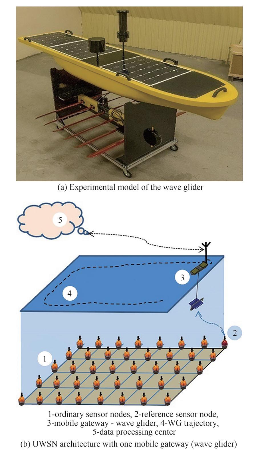Figure  1  Model of the wave glider and UWSN architecture

Download: Full-Size Img

Two variants of sensor placement can be considered, which are determined by the topography of the seabed.

In the first case, the stationary orthogonal grid of sensors is placed on a flat bottom (the presence of various obstacles is not taken into account). This corresponds to the topology of the bottom surface at depths of 1 000 m, which are considered further in the paper. The probability of message delivery is determined only by the distance between the sensors and physical characteristics of the environment, such as absorption and scattering by the water. This probability is the same in all directions (isotropic environment).

In the second, which is a more general case, the same grid is located on the bottom with a complex 3D topology. There may be various obstacles at the bottom - reefs, sunken objects, accumulations of algae, which make it difficult to transfer the message. The type of obstacle determines the probability of message delivery from one sensor to another. Thus, in different zones of the water area, the probability of message delivery will be different (anisotropic environment). The second case is more complex and less representative for analyzing the efficiency of the routing protocols of data forwarding to the gateway with the required reliability.

Therefore, this article considers the first variant of the sensor placement, when the probability of message delivery depends only on the distance and physical characteristics of the medium.

It is assumed that there are one or more dedicated reference nodes to which data from the ordinary nodes in the network is forwarded. Thus, a significantly larger traffic volume passes through the ordinary nodes near the reference nodes and through the reference nodes themselves. Apparently, the more data passes through the underwater wireless network node, the greater is its power consumption. Consequently, there is a problem of imbalanced power consumption in the network. This problem leads to reference nodes failing earlier than others due to battery drain, resulting in a shortened lifespan of the sensor network as a whole. Various energy balancing methods are used to equalize the energy consumption of all nodes in the network:

· Individual selection of the battery capacity depending on the position of nodes in the network and the functions they perform. In this case, the reference nodes can be equipped with high-capacity batteries.

· Different density of network nodes in the water area, depending on the expected traffic intensity. This solution is aimed at ensuring redundancy in the network structure and duplication of the individual nodes' functions. If one network node fails, its functions will be shifted to an available redundant neighboring node.

· Using routing protocols based on such principles as alternating long and short distance transmission and assessing the residual energy value of the nodes on the way to the gateway. In this case, the route in which the nodes have more residual energy is selected from the set of alternative routes.

· Using clustering as division of all network nodes of the UWSN into groups (clusters) with internal routing and internal reference nodes.

· Using the individual network components mobility (mobile gateways). Autonomous underwater vehicles (AUV), underwater gliders (UG) and wave gliders (WG) can be used as mobile gateways.

In this paper a wave glider is used for energy balancing of the network. Let the UWSN be located in a physically homogeneous medium and have the form of a square orthogonal grid with dimension n × n, where n is the size of the grid in terms of the number of nodes. The sensors are located at their nodes. Localization of sensor nodes on an orthogonal grid is convenient because its geometric characteristics are easy to compute. If the network has a single reference node, which is located in the lower right corner of the grid, then summarizing the total number of transmissions of all messages from ordinary nodes to the reference node through the nearest neighbors, we get the following expression:

This is apparently the minimum number of transmissions needed. It will increase if it is necessary to resend messages in the event of losses. It is assumed that an ordinary node is at the k-th range level from the reference node, if k hops are required to deliver the message. Thus, it is convenient to characterize an ordinary node by its range level from the reference node.

Taking into account the message delivery probability, p, and the possibility of sending the message for an unlimited number of times, the mathematical expectation of the number of transmission attempts between neighboring nodes, required for successful delivery is 1/p. The total expected number of transmissions in the network is then defined by the following expression:

Since it is obvious that the bandwidth of a single reference node is limited, and a large value of n will slow down message reception, leading to a bottleneck. In this paper, three different variants of reference node localizations are considered with the aim to improve network bandwidth, and consequently increase network reliability and efficiency:

1) Partitioning the net into a finite number of clusters: in each cluster, ordinary nodes send messages to the reference node, which in turn sends the information to the mobile gateway. In this case, the mobile gateway - the wave glider (WG) - needs to bypass the entire water area, sending notification to the reference nodes to establish a connection and receive messages from them (Figure 2a).

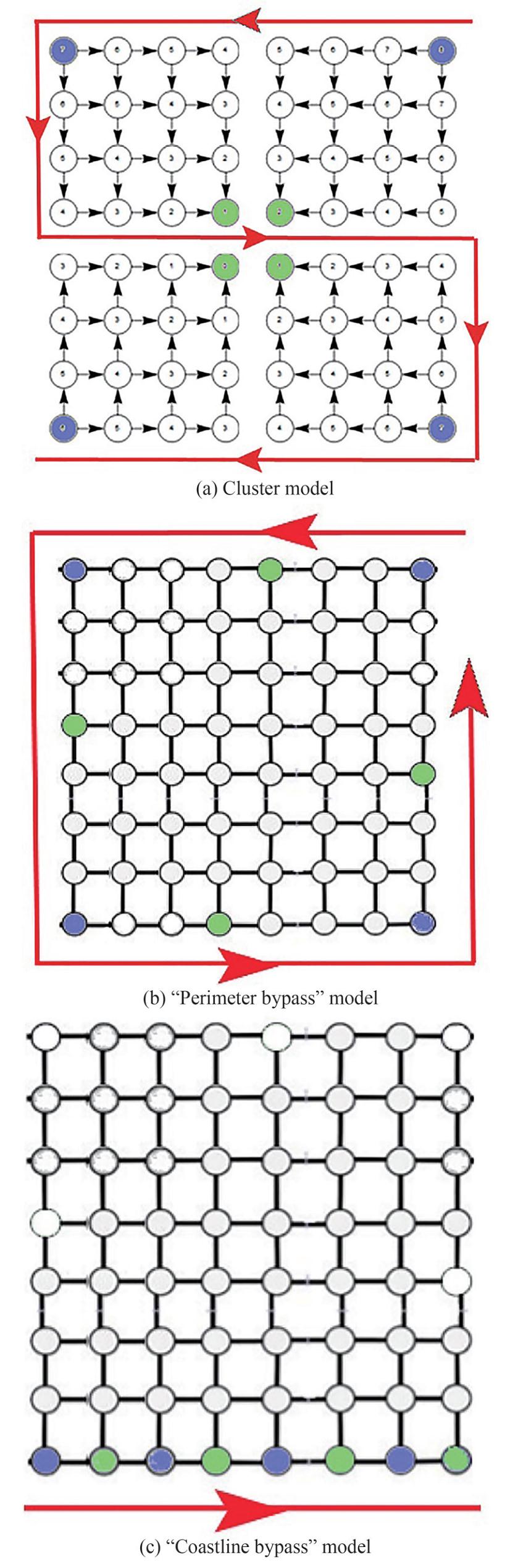Figure  2  The model of the FSGS of 64 nodes with a mobile gateway (wave glider). Red arrow line - trajectory of WG movement

Download: Full-Size Img

2) Reference nodes' location on the perimeter of the water area. The WG should bypass only the perimeter of the water area (Figure 2b).

3) Reference nodes' location along the coastline (one of the sides of the net). The WG should bypass only the coastline (Figure 2c).

3   Physical problem descriptions

This paper deals with the problem in the following model formulation descriptions. Let it be required to measure some characteristics and transmit data (information messages or network packets) from each ordinary node through the other nodes to the reference ones, which are in their turn pass packets to the gateway (Figures 1 and 2). The probability of message delivery between two nearest nodes depends only on the distance between them (r) and is equal to p=p(r). Transmitted packet amount generated by each node is the same. In addition to information on the measured characteristics, the packet contains the necessary service information.

The following physical parameters are used to determine the network characteristics. The total running time of the network between two measurements of the characteristics (cycle) is assumed to be limited and is represented by T. All ordinary nodes must pass the results of measurements (their own and all others') through the reference nodes to the gateway and proceed to the next measurement during this time. In this paper three time-ranges of measurements are considered - once every few minutes, once every hour, and twice a day. The choice of time range is determined according to the network application purposes.

The routing protocols used are neighbor-to-neighbor routing protocols, which means that the ordinary nodes have to pass messages only to their nearest neighbors. If after a fixed number of transmissions to all neighbors the message is not transmitted, it is considered as lost and the node begins transmitting the next message in the queue. The routing table determines which neighbor has a higher, lower or zero priority for transmitting messages for each node. The priorities are determined during the agents' learning process, based on the shortest distance to the reference node and on the number of successful transmissions along the given direction on the previous cycles. Thus, the routing table can continuously be rebuilt during learning. The agent learning algorithms is not discussed since it is not the primary interest of this paper.

The medium access control protocol is non-synchronized hydroacoustic channel access based on competition. The well- known classical ALOHA protocol is an example of such a protocol (Ahn et al. 2011). For energy conservation reasons, the number of reference nodes m is set to 5% of the total number of nodes in the network (Lindsey and Raghavendra 2012):

In addition, the total expected number of transmissions in the network is determined by Equation (2), in which the probability of message delivery between the two nearest nodes is p=p(r).

If L_p (k) is the total expected number of transmissions through one ordinary node at the k-th range level from the reference node, then T_k = T/L_p (k) is the average running time of transmitting of one message and λ_k = L_p (k) /T is the flow of messages through the node during one cycle. The running time of the ordinary node is divided into the following intervals: T_inf is the time duration for data collecting, T_s is the time duration for packet transmission and receipt of delivery acknowledgement. In this work it is assumed that all messages have the same length, and the time of their single transmission is T_s = 0.2 s. The average waiting time between any two consecutive messages is defined as represented by T_w. The energy characteristics of the sensor are:

· P_s = 25 W is the power when sending a message,

· P_w = 0.3 W is the power when waiting for and receiving a message, and

· E₀ = 864 kJ is the capacity of the 12V battery.

4   Mathematical model of the problem

4.1   Lifespan estimates for ordinary and reference nodes

Knowing the initial battery energy E₀ and the power P_k consumed by the node at the k-th range level, the network node lifespan t_k can be estimated as follows:

The node spends energy E_k^c for data collection, energy E_k^s for L_p (k) message transmission, and energy E_k for waiting during one cycle, so the total energy spent per cycle E_k is defined as follows:

Energy E_k^s, which is spent on sending the message, is far higher than the energy E_k^c needed to collect data, so neglecting the energy E_k^c and considering that E_k = P_kT, the expression for the total energy consumed by the sensor per work cycle T will look as follows:

The waiting time T_w can be calculated as the time not taken up by message transmission:

It is not difficult to obtain the sensor lifespan at the k-th range level from Equations (4) and (6):

Substituting the known values of the parameters into Equation (8) and converting them into hours, the following result is obtained:

Equation (9) shows that at $ \frac{{4.94{L_p}(k)}}{T} \ll 0.3$, the lifespan of the node at this range level ceases to depend on the number of packets transmitted, and tends to 800 hours. Let us call such a mode, (at which this condition is met) the low-loading mode, and the mode at which 4.94L_p(k)/T ≈ 0.3 is met, the high-loading mode. If the reference node operates in the low-loading mode, its lifespan will depend very little on localization, and optimization becomes problematic according to this criterion. For this reason, only high loading of the network is considered in the first theoretical part of the paper.

Thus, knowing the node workload and the cycle duration, it is possible to determine their lifespans, and estimate the lifespan of the whole network (by analogy with reasoning (Lindsey and Raghavendra 2012), that the system remains viable, provided that at least 25% of the network nodes are functional).

4.2   Energy costs estimate

The power is assumed to be negligibly small P_w ≈ 0 in message waiting and reception modes, and thus their costs are negligible. This assumption allows isolation of "pure" energy costs of message transmission and to compare different localizations more effectively in terms of the number of retransmissions. The total energy costs of such an "ideal" network are related only to message transmission, which is expressed as:

It should be noted that the higher the network loading, the closer is the considered network to an "ideal" one, since most of the time is actually spent transmitting messages instead of waiting. This again leads us to the necessity to consider only high network loading in the first part of the paper. Dividing the last expression by the total number of nodes in the network, it is possible to obtain an expression for the specific energy cost (energy per node) given by:

Network optimization criteria.

The three models of localization shown in Figure 2-clustering, perimeter bypass, and coastline bypass – are evaluated in terms of two criteria:

· total and specific energy costs of transmitting all messages to the gateway in a single cycle. The network would be regarded as more efficient at lower energy costs;

· lifespan of reference nodes t_ref and of the network as a whole. It is assumed that the longer is the node lifespan, the higher would be the network reliability.

Consider two options for setting the problem:

· Optimization of the operation of the UWSN in water areas for arbitrary scale (construction of a network in which the distance between nodes and the number of network nodes is determined by the probability of message delivery);

· Optimization of UWSN operation in water areas for a specified size (construction of a network for a specified water area size and number of nodes).

5   Optimizing UWSN in water areas of arbitrary scale

The water area is assumed to be unlimited in size and here it is defined as the "sensor network scale". Any number of nodes can be placed at any distance from each other, and therefore with any probability of delivery. It is assumed that the given probability lies in a wide range of 0.5 < p < 1.0. This allows us to consider the entire range of physical conditions - from ideal conditions p=1.0 to extremely adverse ones p=0.5. It makes no sense to consider lower delivery probabilities because they either result in a high percentage of lost messages, or require so many retransmissions per message that the sensor network cannot work properly.

A short cycle of two minutes, i.e., T=120 s, is considered. The calculation results of the dependencies of network efficiency and reliability on sensor localization are given below to determine the optimal one at different scales.

5.1   Clustering usage model

The study of possible reference nodes localizations begins with the variant of cluster localization. The network of n² dimension is divided into m clusters. Each cluster is a network of smaller dimension with side $ l = n/\sqrt m $, there is a reference node marked with a blue circle in one of corner nodes in Figure 3a. Ordinary nodes transmit messages to a reference node in each cluster, which then sends data to a mobile gateway. It is assumed that the same amount of power P_s = 25W is consumed in transmitting each message from the reference node to the glider.

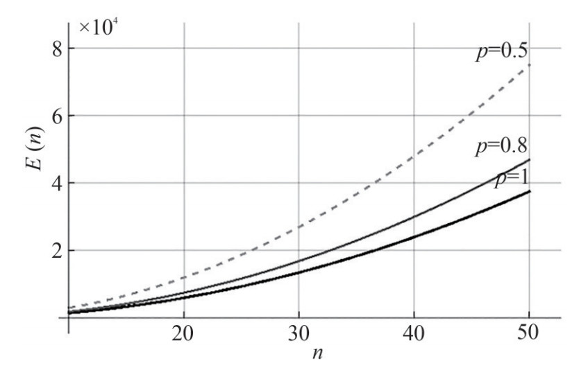Figure  3  Total energy costs versus linear size n of the network for clustering model at different probabilities p of message delivery

Download: Full-Size Img

The dynamic protocol indicates to transmit messages only to the nearest neighboring nodes down and to the right.

It is convenient to calculate the number of transmissions in a cluster L^m from Equation (1) and, multiplying it by the number of clusters, the number of transmissions in the whole system would be:

Based on Equation (3) the number of nodes on the cluster side is independent of the network scale

and can be chosen to be either 4 or 5.

The total number of transmissions in the network, for example, for clusters with side l = 4, i.e., consisting of 16 nodes (Figure 2a) at a given probability of message delivery p can be obtained from the Equations (2), (12) and (13) as follows:

Substitution of this expression into Equation (10) makes it possible to determine the energy cost of message transmission in the case of clustering.

It is easy to see that the specific costs in the case of clustering do not depend on dimension n², but they are proportional to the probability multiplier 3/p. The lower the delivery probability, the higher the unit cost becomes due to the increased number of retransmissions. The total network energy consumption grows depending on its size at different probabilities of the p message delivery is shown in Figure 3. With a high probability of message delivery (p=1), no retransmissions are required and the power consumption is minimal. The lower the probability of delivery, the greater the energy consumption.

Ordinary nodes on the k-th range level must pass their message and all messages from farther levels to the net corner; i. e., the reference node. Obviously, energy imbalance occurs in such a system. To balance the energy, a method is adopted by changing the reference node at each time interval, passing these rights in the cluster alternately to the upper left and lower right nodes of the net, as the least and the most loaded. The blue nodes in Figure 2, a represents the reference nodes in the first cycle, and the green nodes in the second cycle. By performing a simple transformation, it is possible to derive an equation for the number of transmissions from the k-th range level instead of equation for the total number of transmissions in the cluster.

The average node load at the k-th range level in the system for several time cycles at l=4 is determined by the following expression:

Thus, if k=1, the average load of the reference nodes themselves and the flow of messages (traffic) through the reference node per cycle can be determined by:

Knowing the nodes' load, their lifespan can be found, and consequently, the lifespan of the entire network can be estimated by substituting Equation (15) into Equation (9).

Consider a network of 2 500 nodes (linear size n = 50) for an example. Figure 4 shows the nodes lifespan depending on their distance from reference nodes with the cycle time of 2 minutes. The grey shaded area in the graph corresponds to the lifespan of the network or, otherwise, nodes "death time" of levels 1 to 3, i.e., 75% of all nodes in the network.

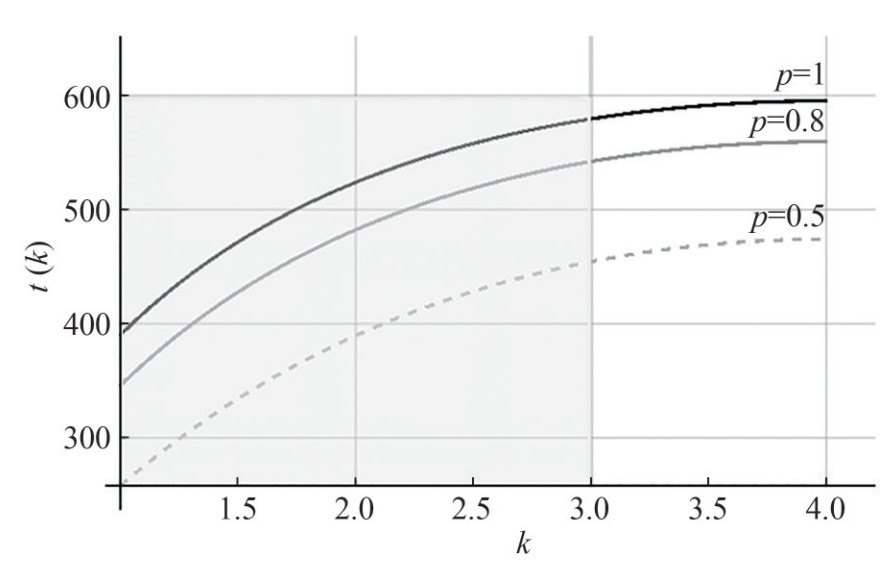Figure  4  Nodes' lifespan at different range levels k for a clustering model for a network of 2 500 nodes with a cycle time of 2 minutes

Download: Full-Size Img

The network lifespan with delivery probability p=1 and cycle time of 2 minutes is approximately 580 hours and does not depend on the size of the water area, but only on the size of the cluster in the considered model.

5.2   "Perimeter bypass" usage model

The next model of FSGS, known as "perimeter bypass" as illustrated in Figure 2b, requires assumption that the reference nodes are the ones located along the perimeter of the water area. Their number can be m = 4 (n − 1) or less, otherwise, all nodes on the perimeter are given rights of reference nodes. The range levels from the reference nodes are the perimeters of the squares nested within the "main" grid square for this localization. Summing up all the transmissions to the reference nodes, the following result is obtained:

If all nodes on the outer perimeter are reference, their load is defined by the following expression:

If only m nodes are reference nodes on each side, the same number as in the case of clustering, namely n²/m can be obtained. The load on the reference nodes increases in this case.

The result is an unbalanced network in terms of energy costs. Balancing is then attained by letting the reference nodes on the perimeter to be selected on the assumption that their total number m is about 5% of the total number of nodes. The method of assigning reference nodes among all perimeter nodes can be close to the LEACH protocol (Mansouri and Ioualalen 2016), which sets a threshold value of sufficient energy to assign a node as a reference one. In this case each node on the perimeter will send to the gateway only a fraction of the messages coming to the perimeter, which is equal to $ \frac{m}{{4(n - 1)}}$ for several operation cycles. Multiplying the reference node load by this fraction returns the process to Equation (18).

We use the neighbor-to-neighbor routing protocol considered earlier (in the clustering problem). The entire network is divided into four triangles, each with its apex in the center of the water area and its base on one of the sides of the water area outer perimeter. The nodes within a particular triangle have information about their location and transmit messages only to the right side. This allows messages to be evenly distributed to the four sides of the perimeter. Consider a dynamic protocol, which indicates to transmit messages first to the nearest neighbor in the direction of the selected side of the perimeter, and, if unsuccessful, to both sides of that direction. The total number of transmissions on the network can be obtained by substituting Equation (17) into Equation (2), taking into account Equation (3)

Substitution of Equation (19) into Equation (10) gives the total energy cost of message transmission in the case of perimeter bypass.

The dependence of the total energy costs for one cycle on the number of nodes (from 100 to 2 500) at different probabilities of message delivery is shown in Figure 5a. When the delivery probability decreases from 1.0 to 0.5, the energy costs are doubled, similar to the clustering case, but the absolute energy costs become much higher, 100 kJ and 200 kJ respectively, compared to 37.5 kJ and 75 kJ for the cluster use model.

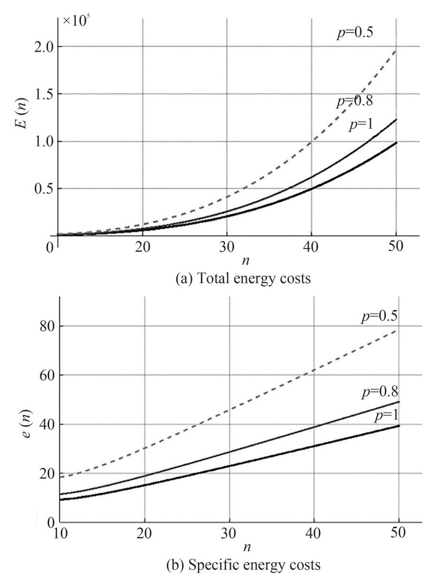Figure  5  Variation of energy costs with linear size n of the network (10 < n < 50) for the "perimeter bypass" model with different message delivery probabilities

Download: Full-Size Img

Substituting Equation (19) into the general Equation (11) determines the specific energy costs of message transmission for "perimeter bypass" model. Figure 5b shows how the specific costs increase as a function of the number of nodes.

By performing a simple transformation, the formula for the number of transmissions from the k-th range level instead of the formula for the total number of transmissions can be obtained:

If k=1 the average load of reference nodes and the flow of messages through the reference node in one cycle can be determined

Knowing the nodes load, their lifespan can be determined and the lifespan of the entire network can be estimated by substituting Equation (20) into Equation (9). Figure 6 shows how the node lifespan grows depending on their distance from the reference nodes with a cycle time of 2 minutes for a network of 2 500 nodes. The grey highlighted area of the graph corresponding to the lifespan of the entire network.

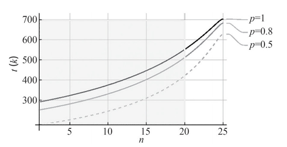Figure  6  Nodes lifespan at different range levels k for the "perimeter bypass" model for a network of 2 500 nodes with a cycle time of 2 minutes

Download: Full-Size Img

5.3   "Coastline bypass" usage model

The "coastline bypass" model of FSGS shown in Figure 2c assumes that the reference nodes are located on the side of the water area that is parallel to the coastline. If the number of reference nodes is still m, then their load is equal to n²/m, as in the previous case. The network is balanced similarly to the perimeter bypass variant, assigning 5% of the total number of nodes as reference. In this case, each node on the coastline will transmit to the gateway only a part of incoming messages equal to $ \frac{m}{n}$ during several cycles. By multiplying the reference node's load by fraction $ \frac{m}{n}$, the following relationship is obtained:

The total number of transmissions on the network is defined as:

Consider a dynamic protocol, which indicates to transmit messages first to the nearest neighbor in the direction to the shore, and in case of failure - in both directions from it. The total number of transmissions per network can be calculated by substituting Equation (23) into Equation (2), taking into account of Equation (3):

Substituting Equation (24) into the general Equation (10) gives the total energy cost of message transmission in the "coastline bypassing" case.

Figure 7(a) shows how energy costs increase depending on the number of nodes. As the probability decreases from 1.0 to 0.5, the energy cost doubles as in the previous cases. However, the absolute values of energy costs become even higher at 300 kJ and 600 kJ, respectively, as compared to 100 kJ and 200 kJ in the "perimeter bypass" model, and 37.5 kJ and 75 kJ in the "clustering" model.

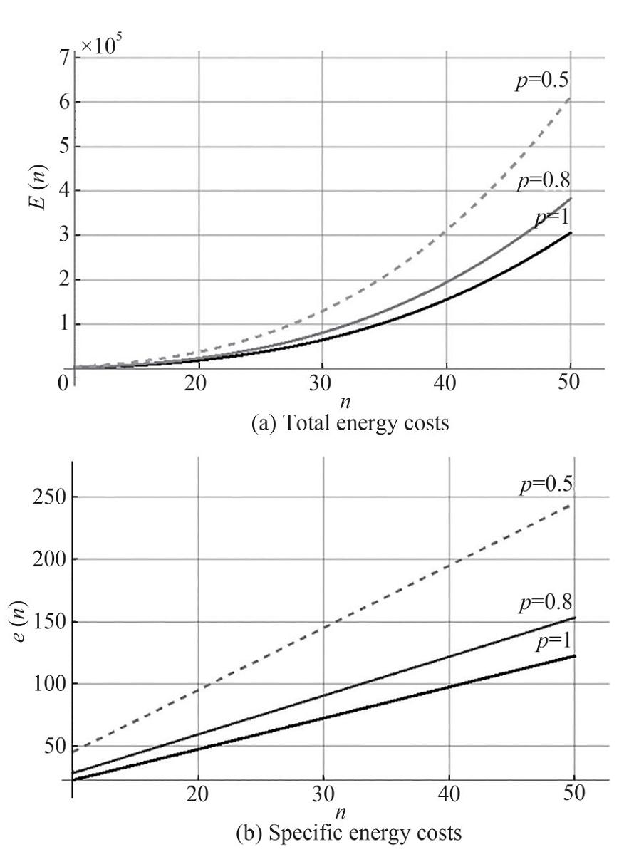Figure  7  Variation of energy costs with linear size n of the network (10 < n < 50) for "coastline bypass" model with different message delivery probabilities

Download: Full-Size Img

Substituting Equation (24) into the general Equation (11) gives specific energy costs of message forwarding in case of "coastline bypass" model, which is depicted in Figure 7b. By performing a simple transformation, the formula for the number of transmissions from the k-th range level instead of the formula for the total number of transmissions can be obtained:

Thus, if k=1, the average load of reference nodes and the flow of messages through the reference node per cycle (assuming that measurements are taken every 2 minutes) can be found:

Knowing the nodes load, their lifespan can be determined and the lifespan of the entire network can be estimated by substituting Equation (25) into Equation (9). Figure 8 shows how the nodes lifespan grows depending on their distance from the reference nodes for a network of 2 500 nodes. The grey highlighted area of the graph corresponds to the lifespan of the entire network.

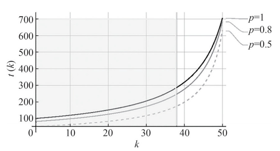Figure  8  Nodes lifespan at different range levels k for the "coastline bypass" model for a network of 2 500 nodes with a cycle time of 2 minutes

Download: Full-Size Img

Figures 4, 6 and 8 show that the lifespan of agents close to the reference nodes is very short (about 100 hours for "coastline bypass", 300 hours for "perimeter bypass" and 400 hours for "cluster"); the lifespan of agents farthest from the reference nodes is much longer–about 700 hours.

When "coastline bypass" the lifespan of various network agents has the greatest difference than for clusters and the "perimeter bypass". Clustering model is the most energetically balanced network structure, and the "coastline bypass" is the least balanced.

5.4   Comparison of the three usage models in arbitrary scale water area

This section compares the proposed variants of localization at different network scales. Consider the energy costs for all localizations separately for small linear sizes (scales) 2 < n < 14 (the number of nodes in the water area will thus change from 4 to 196), and for large linear sizes (scales) 20 < n < 50 (the number of nodes from 400 to 2 500). In addition, the different values of probability of message delivery in the range 0.5 < p < 1.0 is considered. The first case is the "ideal" delivery probability p=1, which, although it cannot be implemented in practice, gives a good idea of the theoretical capabilities of the proposed localization in ideal conditions. And the second case - very low delivery probability p=0.5, which, of course, should be avoided in modeling, but it gives an idea about behavior of chosen network localization in extremely unfavorable conditions.

For the study of the energy efficiency of small-scale networks the results are shown in Figure 9. It is shown in Figure 9 that regardless of the probability p, the "perimeter bypass" model is the most energy effective on small networks. The "clustering" model is close enough to it. The energy characteristics of the "coastal bypass" model are much worse.

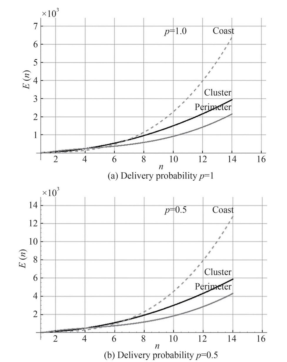Figure  9  Total energy costs E(n) versus linear size (scale) of the network in the range 2 < n < 14 under three different usage models

Download: Full-Size Img

As for large networks, it is shown in Figure 10 that on large networks the "clustering" model is the most energy efficient. The "perimeter bypass" model is somewhat worse, but close enough to it. The "coast bypass" model has much worse energy characteristics. Of special importance is fact that the two models - "perimeter bypass" and "clustering" - are almost identical in terms of energy efficiency on an average scale of the order of n=20.

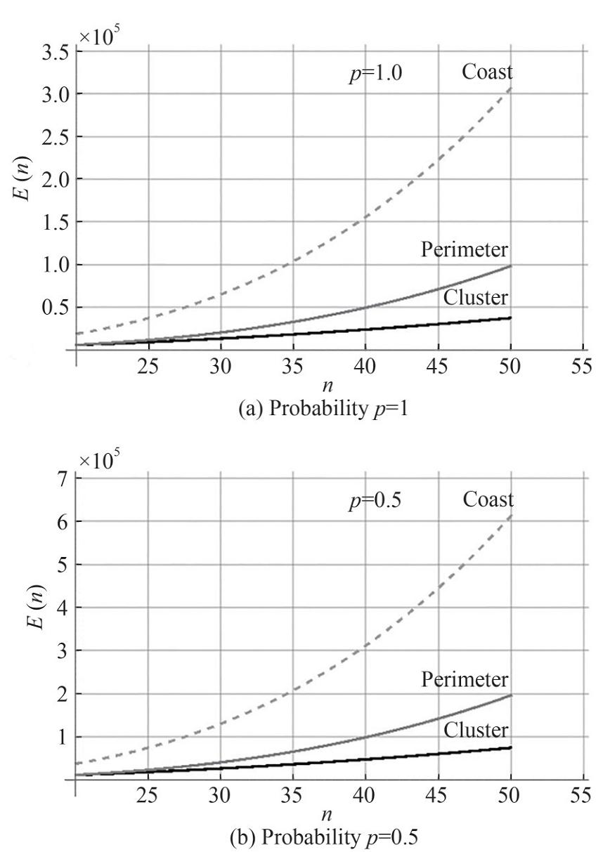Figure  10  Total energy costs E(n) versus linear size of the network (20 < n < 50) for three different usage models

Download: Full-Size Img

With regard to comparison of node lifespan for different models, it must be noted that the fundamentally different structure of the network in different localizations does not allow direct comparison of the nodes' characteristics at the k range levels. The only universal value, independent of the localization and characterizing the reliability of the system, is the lifespan of the reference nodes.

Shown in Figure 11 are the comparisons involving small- scale networks reliability. It is depicted in the figure that the "perimeter bypass" model is the most reliable on small networks in terms of lifespan. Coast bypass is reliable on very small networks (less than n × n=64 nodes). Obviously, it is also shown in the figure that the reliability of the "clustering" model does not depend on the network size at all.

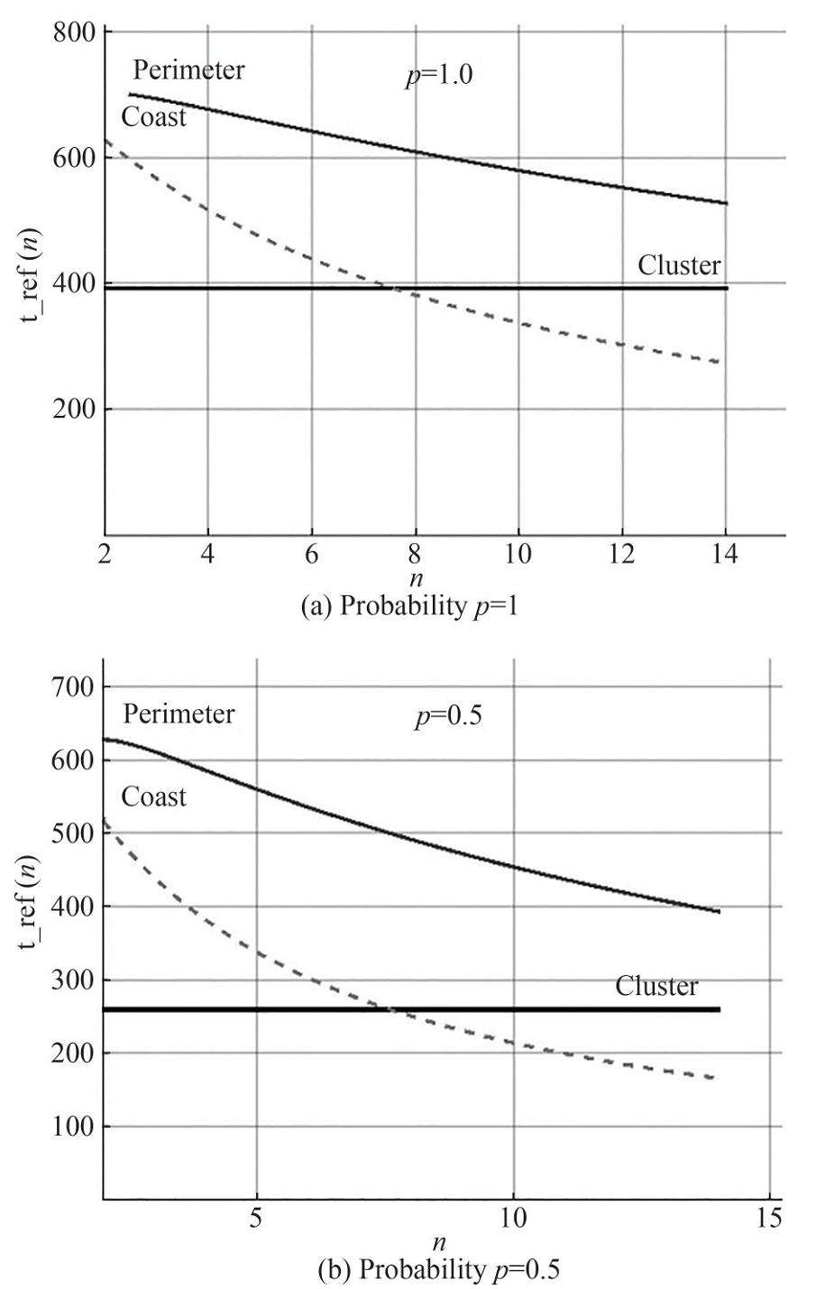Figure  11  Reference node's lifespan t_ref (n)) versus linear size of the network (2 < n < 14) for three different usage models for a cycle time of 2 minutes

Download: Full-Size Img

Comparison of Figure 11a and Figure 11b shows that, first, the qualitative character of the dependencies does not change when the delivery probability changes. Secondly, the lifespan of the network is less sensitive to the delivery probability than the energy efficiency.

The results for the large networks are presented in Figure 12, which shows that in terms of lifespan the "perimeter bypass" usage model is still the most reliable on large networks with n < 30. The situation changes at n > 30. On very large networks, "clustering" usage model is the most reliable; the "coastline bypass" usage model is less reliable.

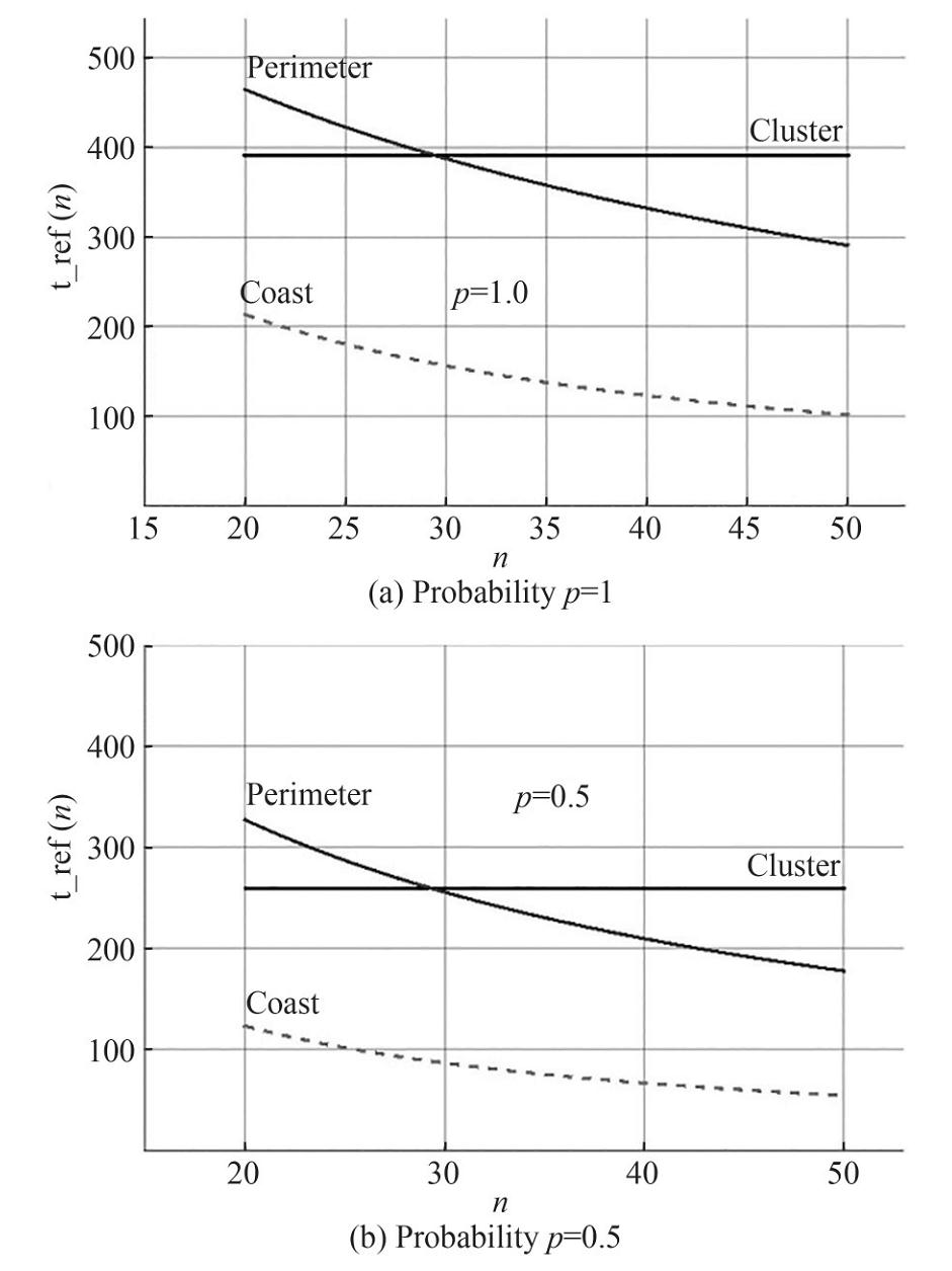Figure  12  Reference nodes lifespan ref (n) versus linear size of the network (20 < n < 50) for three different usage models

Download: Full-Size Img

A quantitative comparison of the localizations/usage models discussed above is presented in Table 1. The best characteristics are highlighted in bolded texts in the table. The table shows that "clustering" usage model for an arbitrary unlimited water area has the best characteristics for large networks. On the other hand, the "perimeter bypass" usage model has the best characteristics for small networks.

It is important to note here that when solving real problems in a given finite water area, the simplifying assumptions made above are not quite correct. Firstly, changing the number of nodes will change the delivery probability in a finite water area. Secondly, it is necessary to match the cycle duration with the frequency of the wave glider bypassing the water area when solving a real problem. This means that the waiting time T_w between successive transmissions cannot be neglected. In addition, it is necessary to consider the various intervals of data collected by the sensors for a complete picture of the possible states of the network. This is performed in the next section.

6   Optimization of UWSN within limited water area

If the size of water area, where the sensor network should be located, is specified in advance, the number of sensors would be proportional to the distance between them. The more sensors in the water area, the higher the probability of message delivery. Thus, the probability p cannot be an input parameter, but is a function of distance p (r). In this work, a wide range of probability is considered: 0.5 < p (r) < 1.0.

The results of the computational simulation to analyze dependences of the network efficiency and reliability on the distance between nodes at the given scale of a network are presented here. They allow determination of optimum localization in the given water area, i.e., the optimum distance between nodes and probability of messages delivery.

The data in the network is collected by a wave glider, which moves along a specified route, from all nodes that at least were once the reference. Let the velocity of the wave glider be v = 0.7 m/s for the model estimation. Then the waiting time between message transmissions begins to play a significant role, because it determines the frequency of data collection by the glider, which is related to its speed. Therefore, it is reasonable to consider the three time ranges of data collection by the sensors (cycle time T) specified above and compare them with the time spent by the glider to bypass all reference nodes.

6.1   Comparison of characteristics

The probability of message reception, depending on the distance between the receiver and transmitter, is defined by the Neumann-Pearson theorem according to the following relationship:

where SNR (r) is the signal-to-noise ratio at a distance between the nodes:

Let the signal-to-noise ratio at distance r₀ = 1 m be equal to SNR₀ = 2 000 in a given water area, frequency, and hydrometeorological conditions.

The losses associated with acoustic energy attenuation are usually characterized by the coefficient of energy attenuation due to signal absorption and scattering by the medium (water absorption coefficient β), expressed in decibels per km (Sheehy and Halley 1957). For low absorption and scattering by the medium (LM) - the absorption coefficient is equal to β=0.036×10⁻³, for middle (M) − β=0.90×10⁻³ and, for high (HM) − β=0.90×10⁻³.

Graphically, the probability of message delivery depending on the distance has the profile shown in Figure 13. The graph on Figure 13 marks the area of change of the message delivery probability in the range 0.5 < p < 1.0. The graph shows that to hit the range 0.5 < p < 1.0. in the water with low and middle β, it is necessary to place sensors at distances 500 < r < 2 500 m, and in the water with high β - at distances 500 < r < 1 500 m. Placing the sensors at shorter distances will not give any gain in terms of improved reliability, as the 100% delivery probability has already been reached. It does not make sense to place sensors at longer distances, because the delivery probability at those distances is extremely low, p < 0.5. These preliminary estimates are used later in analyzing the simulation results.

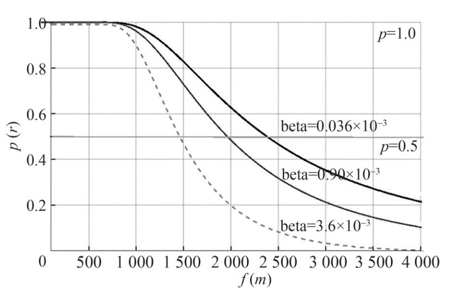Figure  13  Probability of message delivery versus distance for different absorption coefficient β

Download: Full-Size Img

It is necessary to proceed from the given reliability requirements when determining the optimal network configuration. Let us take three variants of sensors placement, providing: (ⅰ) absolute reliability (800 m from each other), (ⅱ) average reliability (1 100 m) and (ⅲ) extremely low reliability (1 700 m). The data on delivery probabilities for these placements is obtained from the graph in Figure 13 and is summarized in Table 2.

Now we determine the optimal configuration of the network in the water area of given dimensions. It is assumed here that a number of stationary nodes are placed at the bottom of the water area of size R×R for data collection, which is sent to an onshore processing center using a wave glider (mobile gateway). The distance between the nodes is equal to r. The water area is S=144 km² (with side R=12 km) for an example. The number of nodes is related to the distance between them by:

The wave glider sends a command to begin message transmission during movement along the specified route and upon entering the "visibility zone" of a particular reference node. It is assumed that the considered water area has low depths of up to 1 000 m, so the message transmission in the vertical direction from the reference node to the wave glider is carried out with high enough probability. In this case, due to the fact that the wave glider moves along a given route at a relatively low speed (0.2−1.0 m/s), the packet can be transferred by the reference node in the direction of the gateway so many times as to ensure guaranteed delivery of the message. The glider needs to move between the reference nodes along some "optimal" path, which is generally a separate problem similar to the traveling salesman's problem. The simplest route, assuming that the glider starts from the upper left corner and sequentially bypasses all the reference nodes of clusters, is proposed in case of clustering. The total time of data collection by the glider from all nodes (the time of single bypass of the water area) is the sum of the time spent for $ (\sqrt m + 1)$ movement horizontally and the time spent for movement downwards (see Figure 2a). Taking into account that the side length is equal to (n − 1) r, and taking into account of Equation (3), it is possible to obtain the expression for the total time of data collection from reference nodes:

If the wave glider bypasses the perimeter of the water area, the nodes send messages from the center to the perimeter, Figure 3b. Then the total time for data collection from all nodes (time of a single bypass by the wave glider of the water area perimeter) can be calculated by:

However, if the glider bypasses the coastline of the water area (Figure 3c), then the total time for data collection from all nodes during a single bypass is determined by:

Substituting the numerical values into Equations (30), (31) and (32) at glider speed v=0.7 m/s, it can be concluded that the glider needs about 4.8 hours for the "coastline bypassing" model, 9.2 hours for the "perimeter bypassing" model, and finally, the reference node bypass time (in hours) for the clustering model will depend on the number of clusters m in the water area as 4.8 $ (\sqrt m + 2)$.

The network configuration parameters are summarized in Table 3, where (1) is clustering, (2) is perimeter bypass and (3) is coastline bypass. The table shows that the high loading of the network, which is presented in detail in the previous section, must now be abandoned as it doesn't correlate with the time spent for the glider to bypass the water area. Modeling an "ideal network" without taking into account the speed of the glider turned out to be unsuitable for the real case. It can be expected that the most suitable case for study would be medium UWSN load, namely at once per hour.

Let us take integral characteristics, which now depend on distance between sensors, as main criteria of network optimization. The total energy cost of the network can be obtained from Equation (10):

The lifespan of the reference node - from Equation (9) is:

Equation (33) represents energy consumption of the given size network at different sensor localizations, Equation (34) shows the lifespan of reference nodes (as most overloaded nodes in the network) at different sensor localizations. Using the resulting Equations, compare the three localization models in the next section.

6.2   Energy costs in three UWSN usage models for a given water area

The dependence of the total energy consumption of the network Е (r) for message transmission per cycle, represented by Equation (33), in the water area of S=144 m² with low LM and middle M absorption coefficient β of medium for three considered localizations (cluster model, "perimeter bypass" model and "coastline bypass" model) on the distance r between nodes are shown in Figure 14(a).

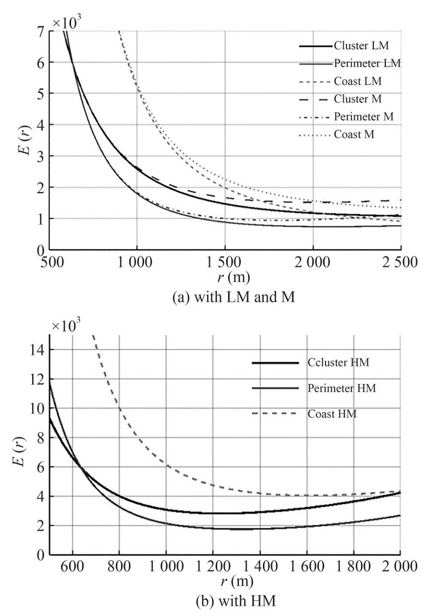Figure  14  Total energy costs of the network in the water area of S=144 km²

Download: Full-Size Img

First of all, it should be noted that no matter which localization of nodes is considered, the total energy cost per cycle has a minimum. This is due to the fact that at small distances r between the nodes, their number is very large and a significant number of retransmissions are required in order for the message to be delivered to the gateway. Therefore, the energy costs are quite high in the region of small r. As the distance r increases, the number of retransmissions decreases and the energy cost drops, but at larger distances the energy cost will increase again, because the probability of successful message delivery decreases and a large number of the retransmissions from the node to its neighbor is required.

This property can be more clearly seen in the graph of the total energy costs of the network to send messages in the water area with HM (Figure 14b). In this case, the minimum is clearly seen in the considered range of r. Indeed, in the case of clustering model, the energy costs turn out to be equal and are about 4 000 J at distances of 800 m and 1 900 m. This is quite a large cost. However, the reasons for this are different – at small distances they are due to the fact that there are a large number of sensors placed in the water area and the path to the reference node consists of a large number of hops. Each hop requires an energy expenditure. At large distances, however, the situation is the opposite – there is a small number of sensors at large distances from each other in the water area. To successfully transmit a message, it must be sent many times from sensor to sensor. This again requires energy expenditure. The minimum lies in the middle between these extreme cases. In this example it is achieved at distances of 1 200 m and the required energy is about 3 000 J. The perimeter bypass model is energetically optimal in the considered water area.

6.3   Time dependencies in three UWSN usage models for a given water area

To analyze reference node lifespan for three variants of localization it is necessary to analyze the influence of frequency of data collection by the sensor network, i. e. to consider two possible ranges: once in 1 hour, and once in 12 hours. Equation (34) is used to analyze the lifespan of the reference node for the three considered localizations. For example, data is taken every hour, and the results are depicted in Figure 15.

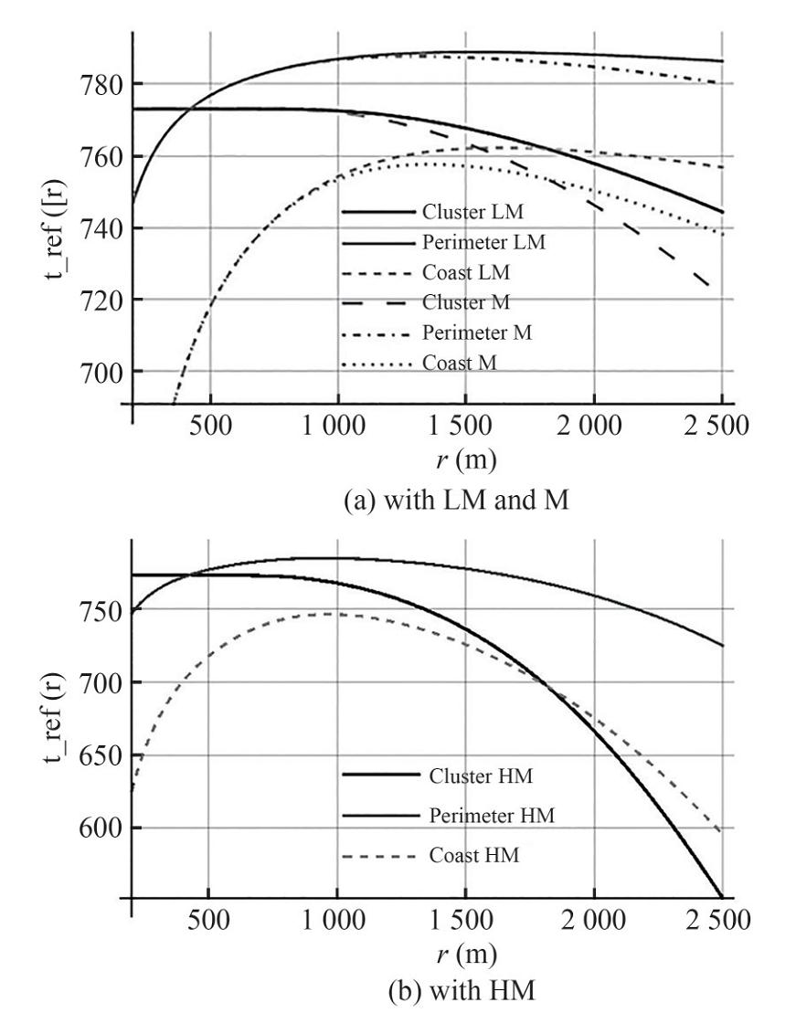Figure  15  Lifespan of the reference node in the water area of S=144 km² when collecting data every hour

Download: Full-Size Img

It is revealed from Figure 15 that the lifespan of the reference node has a maximum. The reasons for this are the same as for the minimum of energy costs. The clustering model has some peculiarity. The curve of reference node in clustering model has an asymptote, to which the graph tends at small distances. The presence of such an asymptote is due to the fact that the loading of the reference node at a fixed cluster size does not depend on the number of nodes in the water area and stops changing when the 100% delivery probability is reached. This always occurs at 800 m. For other localizations, reference node loading increases as the number of nodes in the water area increases even when the delivery probability is one hundred percent.

The maximum is more pronounced and is achieved at about the same distance between nodes - about 1 000 m for the "perimeter bypass" model and "coastline bypass" model, and at 800 m for the clustering model in water with high absorption coefficient β. The perimeter bypass model provides maximum reliability in the given water area.

If measurements are made once every 12 hours (twice a day), the maximum lifespan of the reference node becomes much less pronounced. This is due to the fact that the lifespan is now significantly affected not only by the number of transmissions, but also by the waiting time between transmissions, which increases for any localization. The network becomes more robust and less sensitive to the choice of localization type.

Generally speaking, Equation (34) shows that from some T, optimization with respect to the time criterion becomes impossible, since the lifespan of the reference node tends to 800 hours, regardless of the usage model. Dependence of the reference node lifespan on the interval between measurements for the optimal distance between nodes (chosen as 1 700 m) for water area with low absorption coefficient β is shown in Figure 16. Figure 16 shows that the reference node lifespan does not exceed 800 hours for all localization models. This corresponds to the standby time without packet forwarding.

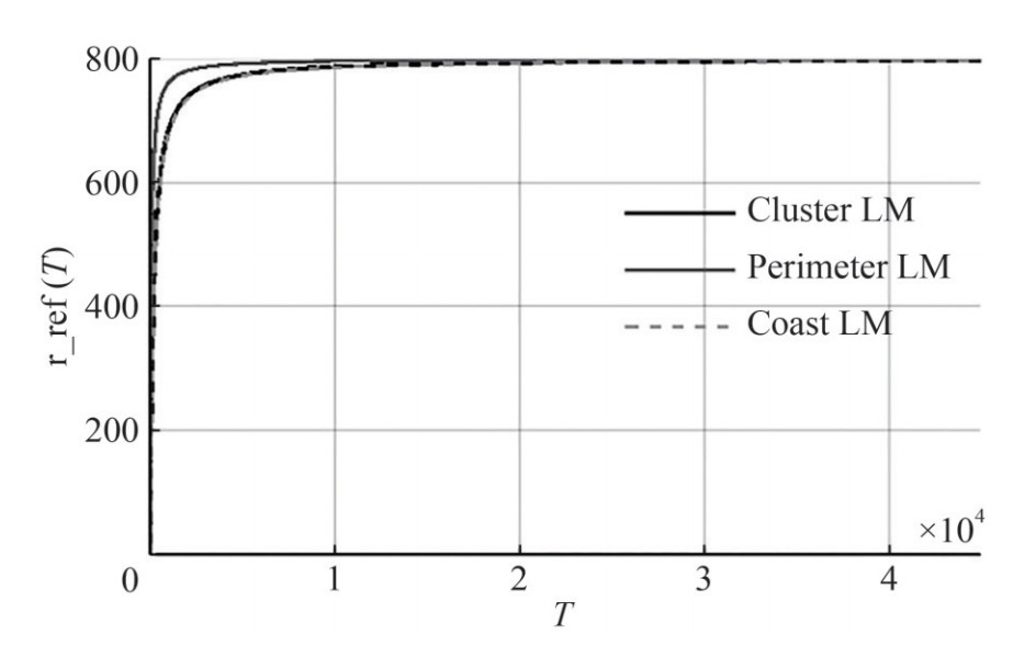Figure  16  Reference node lifespan versus time between measurements in the water area of S=144 km² with low absorption coefficient β when the nodes are placed at a distance of 1 700 m from each other

Download: Full-Size Img

Consider the solution of a real problem of designing an optimal hybrid UWSN with a mobile gateway, the role of which is performed by the WG, for given design parameters as an example. As highlighted before, the UWSN, measuring the physical characteristics of the medium by bottom sensors with a frequency of once per hour, in the water area of S=144 km² and depth of 1 000 m with known (low) muddiness (packet delivery probability equal to p=0.97) is considered.

It follows from the results obtained above that the sensors should be located in the nodes of the orthogonal grid at distances r=1 100 m from each other in order to provide the required probability. Under this condition the total number of sensors in the water area will be equal to n² (r) = 144 km². For energy optimization and increase in network lifespan it is necessary to choose the "perimeter bypass" model. In this case, the total number of sensors on the perimeter, alternately performing the role of reference nodes, will be equal to 44. The load of reference node can be now calculated, which turns out to be on the average 3.27 messages per cycle for given parameters. Then, if data is collected hourly by sensors, then the last reference node will accumulate 62.7 messages during a single waveglider bypass of the perimeter (19.2 hours).

Taking into account the technical features of the modem, let us assume that it can confidently receive/send messages within a cone with an angle of α = 60°. From the location of sensors, it is easy to determine that the glider at the design speed can continuously take data from the sensors moving along the perimeter of the water area. In this case, the WG have an average of about 25 s to receive one message. If, for any reason, several retries are required to receive a message from the reference node, they must be performed within the specified time interval.

This example of the hybrid UWSN architecture shows that a wave glider for relatively small water areas is a promising mobile platform that effectively acts as a gateway for retransmitting data collected in the underwater segment of the network to data centers.

7   Conclusions

This paper analyzes the main functional characteristics of three different localizations of sensor nodes for the model of using the UWSN with a mobile gateway, the role of which is performed by a wave glider. The mathematical apparatus, based on the probabilistic approach, allows to estimate the energy characteristics of the considered UWSN communication architectures, namely to determine the total energy costs of the network for message transmission and the network nodes lifespan. In this case, a simple dynamic "neighbor-to-neighbor" protocol based on competitive access to the environment is considered as an MAC protocol in model problems. Due to the fact that the applied problems solved by the UWSN have different requirements for the network design parameters, a wide enough range of changes in such parameters as: water area size (network scale); required number of sensor nodes located in a specific water area; frequency of data collecting from sensors (cycle time); physical characteristics of the environment are considered to find the optimal solution. The paper considers three models of using the WG for servicing underwater network segment: clustering model, water area "perimeter bypass" model and "coastline bypass" model. The indicators of power efficiency and reliability depending on the above-mentioned design parameters are studied for the nodes of the underwater segment of the network within these models.

Analysis of the simulation results leads to the conclusion that the clustering model of nodes localization has the best performance and reliability characteristics for large- scale networks. On the contrary, for small-scale networks, the "perimeter bypass" model of the node localization has the best characteristics.

It is shown that for all considered localizations there are extremums (minimum) of dependences of the network total energy costs on the distance between nodes. And there are also extremums (maximum) of dependences of the reference nodes lifespan on the distance between nodes for all considered locations, except clustering model.

These results allow determination of the optimal placement of nodes for water areas with known physical characteristics of the medium to obtain the best reliability and efficiency. The presented model example of designing an optimal UWSN with a mobile gateway for a water area of a specific size shows that the "perimeter bypass" use model is practically feasible, energy-efficient and reliable for the case of data collecting by a sensor once per hour on a relatively small water area of 144 km². Under the accepted assumptions, the wave glider is able to reliably serve the underwater segment of the network and transmit data to the processing center. The WG has enough time to receive the messages accumulated by reference nodes (on average, about 25 s for every message) in the mode of continuous motion for depths of about 1 000 m. These conclusions confirm the fact that the WG can be used in practice as a mobile gateway of the UWSN with stationary bottom nodes.

The results obtained in the work show the need for further research based on the proposed probabilistic model of the hybrid UWSN taking into account: the spatial and uneven placement of sensor nodes in the water area, the spatially variable probability field of signal transmission.