1   Introduction

The shipping industry is constantly seeking ways to improve the ship energy efficiency either for economic reasons or for regulatory reasons arising from example from IMO's initial strategy for the reduction of Greenhouse Gas emissions by at least 50% by 2020, compared to 2008 levels (IMO, 2018).

Several design and operational solutions have been proposed. Bouman et al. (2017) and Brynolf et al. (2016) provide a detailed presentation of the energy reduction potential achieved by technical and operational solutions. The first category concerns mainly affecting ship design such as hull form optimisation, implementation of energy-saving devices and waste-heat recovery, while the second category targets solutions involving optimal operation of the ship like weather routing, speed optimisation and preventive maintenance.

Within design solutions, a popular choice is the installation of energy-saving appliances involves installations that are positioned at the area of the ship's propeller, aiming to increase its efficiency and, thus, the vessel's overall propulsive performance. Such upgrades include the Kort nozzle, the wake-equalizing duct, the Mewis duct, the Schneekluth wake equalizing duct, the pre-swirl stator, the propeller boss cap fin and other (e.g., Schneekluth and Bertram, 1998).

Among the above technologies, a popular choice is the Mewis duct, which is a hull appendage with an integrated fin system located forward of the propeller, mounted in its inflow region. It has been introduced in the industry since 2010, and usually used in tankers and high block coefficient ships as an energy-saving device to improve the propeller's efficiency. Its operation relies on three main principles (Schneekluth and Bertram, 1998):

· Wake field equalization: The duct strengthens and accelerates the hull's wake into the propeller and also produces a net forward thrust.

· Reduction of propeller hub vortex: An improved slipstream behind the duct significantly reduces the hub vortex with corresponding thrust deduction, leading to improved thrust and better inflow to the rudder.

· Contra-rotating swirl: Due individually placed fins a preswirl in counter direction is generated, recovering the rotational energy from the slipstream and reducing the rotational flow losses of the propeller.

In summary, the Mewis duct provides with a better streamlined and directed flow into the propeller, reducing its losses and therefore improving its efficiency. The power savings offered vary from 2%, for multipurpose vessels, up to 8%, for tankers and bulk carriers (e. g., ABS 2013, IMO 2016). Additional advantages of the Mewis duct include the low installation time (approximately 4 days), the reduction of cavitation and vibrations as well as that it requires no service. However, its potential is subject to various factors that constitute the ship's hydrodynamic profile and, therefore, each vessel should perform individual hydrodynamic analysis implementing CFD and/or model tests before installing the Mewis duct to evaluate its actual efficiency.

Nevertheless, for several reasons, operators still need to measure and verify the claimed gains during the real operation of a ship when conditions can differ extensively from the design ones. This study aims at the evaluation of a duct's efficiency from a different perspective, focusing on the performance assessment of the operation of the duct. In principle, performance monitoring involves measuring various physical quantities that affect a vessel's performance by onboard sensors with pre-arranged frequency and for a defined amount of time. As a result, a database that characterizes the vessel and its operation under different scenarios and conditions is created. The real-time data describe the vessel's behavior under various circumstances and can, thus, be used to evaluate the effect of these circumstances or events on the vessel's performance. As suggested by Hasselaar (2010), performance monitoring offers multiple benefits as it facilitates the assessment of the hull and engine condition, it evaluates the ship's design by comparing the true operational parameters with the designed ones and it optimizes the sailing performance as the true, optimal and ship-specific operation point can be found.

In the current paper, we utilize performance monitoring to quantify the fuel savings for an Suezmax crude oil tanker with summer deadweight of 158 000 t (called vessel 1) fitted with a Mewis duct during a dry-dock. Specifically, we utilize high-frequency data gathered before and after the installation of the Mewis duct to assess its actual, real-operation impact on the propulsive performance. It shall be noted however that the Mewis duct is installed during a drydock, as a retrofit, where hull and propeller cleaning were also occurred. So, a question arises related to which part of the improvement is owned to the Mewis duct and which to the hull/propeller cleaning. In addition, there was lack of operational data after the previous drydock. Therefore, our analysis will also consider a sister vessel (called Vessel 2) that did not had a duct installed and whose performance will be monitored the same period, to provide with a solid comparison that underlines the long-term effect of the Mewis duct.

An overview of the proposed procedure for the evaluation of the Mewis duct efficiency is presented in Figure 1. Firstly, real-time operational data are collected, by a variety of sensors and measuring devices. Section 2 describes the processing phase of the initial dataset including the application of several filters and the identification and removal of statistical outliers. This phase concludes with the final dataset of the operational data to be used for the performance analysis. Then, the analysis proceeds in two directions. Section 3 examines duct's effect through a set of appropriate Key Performance Indicators (KPIs) which target at monitoring of the vessels' performance in time. The second approach concerns the development of a multiple linear regression model to provide predictions about the fuel oil consumption (FOC) for different operational scenarios (Section 4). The KPI calculation and the regression analysis are two different approaches for evaluating the duct's efficiency and a discussion on their findings is provided in Section 5.

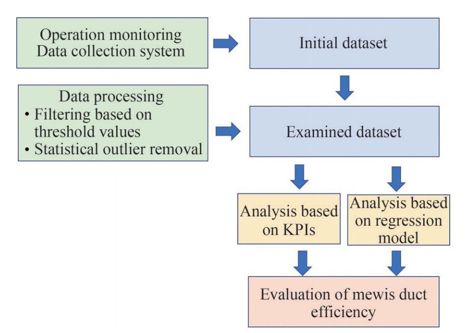Figure  1  Flowchart of the proposed study

Download: Full-Size Img

2   Data analysis

2.1   Set-up of the data collection

The basic characteristics of the examined sister vessels are shown in Table 1. Moreover, the monitored physical quantities, which constitute the parameters of the problem under study, are presented in Table 2. The sampling frequency was 15 minutes, while the total time duration monitored was 3 years for both vessels.

The key time periods examined are the following: Vessel 1:

1. Period 1A: Before the propeller polishing (about 3 months)

2. Period 1B: Between the propeller polishing and the drydock (about 4 months)

3. Period 1C: After the dry dock (duct operation) (about 29 months)

Vessel 2:

1. Period 2A: Before the dry-dock (about 10 months).

2. Period 2B: After the dry-dock (about 26 months). The main events that affect the performance are:

· Dry-dock: a repair process which includes the cleaning of the hull. As a result, the ship's resistance is reduced, and its propulsion performance is improved.

· Propeller polishing (only for Vessel 1): a repair which greatly improves the propeller's efficiency and, thus, the overall performance of the vessel.

· Duct installation: a fitting procedure that aims at improving the propeller's efficiency.

For the analysis to be more accurate and solid, the initial data need to be properly processed in order reduce bias and possible outliers. By omitting values that are not in accordance with most data points, a reliable dataset can be created and used as the basis of the KPI analysis and the regression model, whose aim is to evaluate the impact of the Mewis duct on performance.

The data filtering is achieved through the application of specific filters that accurately identify and reject the "undesirable" parameter values. As the analysis is time-bound, it should be noted that in case a single parameter value is considered "undesirable" then all the other parameter values measured at the same instance will be automatically omitted. Despite disregarding possibly "desirable" values, due to the large size of the initial dataset (approximately 100, 000 data-points for each vessel), the remaining dataset is adequate for the analysis of the examined period.

The histograms of the STW and EP variables for both vessels are shown in Figure 2 and Figure 3, providing a direct visualization of the data range of these parameters. The examination of the histograms is essential for the first part of the filtering procedure, as it can reveal "undesirable" data areas.

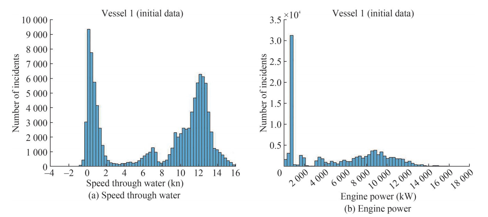Figure  2  Initial data-Histograms (Vessel 1)

Download: Full-Size Img

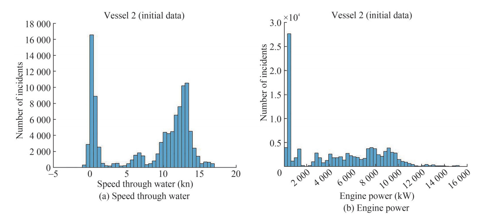Figure  3  Initial data-Histograms (Vessel 2)

Download: Full-Size Img

2.2   Data pre-processing-part Ⅰ: threshold values

The first part of the filtering process sets minimum threshold values targeting at the exclusion of values with no physical meaning, such as negative fuel consumption, which is the result of sensor malfunctioning. Furthermore, data related with low ship speed values, measured during port operations and cargo handling, are also omitted. Such data cannot accurately represent the relationships among the physical quantities and thus, are excluded from the dataset by using respective filters. The implemented threshold values are presented in Table 3.

2.3   Data pre-processing-part Ⅱ: outlier detection

The second part of the filtering process aims at the identification and removal of statistical outliers. To achieve that, the relationships among the physical quantities are utilized. Firstly, the correlations among the variables are calculated, so that their co-dependency can be assessed. Afterwards, highly correlated variables are paired and filtered according to the following procedure (Karagiannidis and Themelis, 2021):

1. Choose a primary parameter X

2. The parameter values are divided into groups (Gi) of range v.

3. A secondary parameter Y, which is correlated with the primary parameter X, is chosen.

4. For each Gi group of X, the mean, m_Yii, and the standard deviation, σ_Yi, of the respective Y values are calculated.

5. An outlier threshold value k is defined, which multiplied by σ_Yi, designates the "outlier threshold"

6. If the inequality |Y_ij − m_Yi | ≥ k·σ_Yi is fulfilled, then the Y_ij data point is omitted, along with the rest measurements of the other parameters at the same timestamp.

Finally, once the impact of each X, Y pair (filter) is evaluated, an optimal combination of filters, shown in Table 4, is chosen and applied to the dataset, leading to the final dataset. The values of the outlier threshold k and of the range v were selected after some experimentation keeping in mind to use a k value for each X, Y pair, which accompanied with an appropriate small range, will be able to capture the outlier values.

The impact of the bipartite filtering procedure is depicted in Figure 4. The blue data points are the ones omitted by the thresholds set at the first part of data pre-processing while the red data points are eliminated by the second part. Finally, the green data points are the remaining data that form the final, filtered dataset.

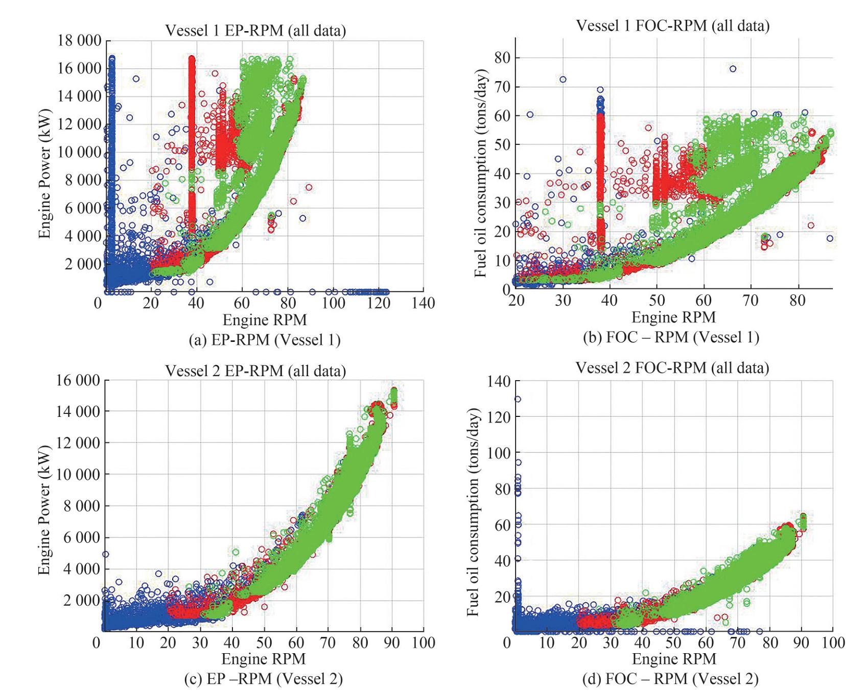Figure  4  Scatter plots. Blue dots correspond to the data points filtered due to threshold values (part Ⅰ), while the red one to the points identified as statistical outliers (part Ⅱ). As green shown the final dataset

Download: Full-Size Img

The graphs of Vessel 1 reveal the existence of 3 main operational regions, which correspond to different propulsion conditions due to, for example, hull and propeller fouling or weather effect. The curves contain valuable information concerning the vessel's performance and thus should not be eliminated during filtering. As far as Vessel 2 is concerned, its depicted curves show no significant outlier regions and, thus, the filters' impact on its data points is limited. Table 5 presents the percentage of data removed at each stage of the filtering process.

3   Analysis based on KPIs

3.1   KPIs definition

Changes in the performance level of the two vessels over the various operational periods can be monitored through suitable Key Performance Indicators (KPIs). Having in mind the type of the performance related with the Mewis Duct, the following KPIs are calculated and analyzed over the monitoring period:

· KPIa = EP/RPM³: It corresponds to the propeller curve coefficient (e.g., Logan, 2011, Themelis et al., 2019). When the KPI's value decreases, the vessel's performance increases since less power is required to maintain constant shaft's revolutions (constant denominator) and greater rpm can be achieved for the same level of power (constant numerator).

· KPIb = STW/FOC: It expresses the fuel efficiency (e. g., Petersen et al. 2012, Aldous 2015). When the KPI's value increases, the vessels performance also increases since for the same amount of consumed fuel by the main engine, higher speed through water is achieved (constant denominator) and for the same speed value less fuel is required (constant numerator). As this KPI is affected by the ship's loading condition, it calculated separately for two reference conditions (ballast and laden).

Before the KPI analysis is performed, three additional data pre-processing actions are applied to the dataset to improve the KPI calculations (Figure 5). The first one aims at reducing the variance of the draft values by keeping only those that lay around the two reference values (ballast and laden drafts). The second one limits the effect of the weather on the dataset by applying filters on the wind speed and the rudder angle. Finally, the engine power and the fuel oil consumption are both corrected by using the Admiralty Coefficient (Themelis et al., 2018).

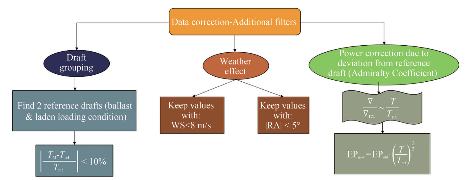Figure  5  Additional filters and corrections for the KPI analysis

Download: Full-Size Img

The draft correction is depicted in Figure 6 for both vessels. The blue points are the ones that lie within the 10% threshold while the black ones are those that are omitted. The reference drafts are shown in Table 6.

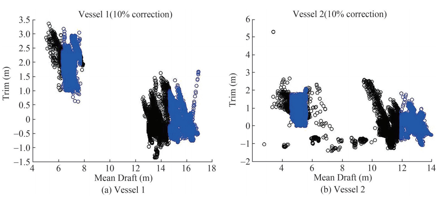Figure  6  Trim-Draft (10% filter). Black dots correspond to the omitted data points

Download: Full-Size Img

3.2   KPIs calculation and discussion

Once the additional filters are implemented, the two KPIs are calculated for both vessels over the examined period. Finally, a comparison between the two vessels is performed aiming to assess the duct's impact on performance. The moving means of the KPIs along with their trend lines are shown in Figures 7-9. During the fact that the post-dry-dock period examined exceeds two years, the results and respective discussion are grouped by two yearly time durations, thus they will be mentioned as the 1^st and 2^nd year after the drydocking.

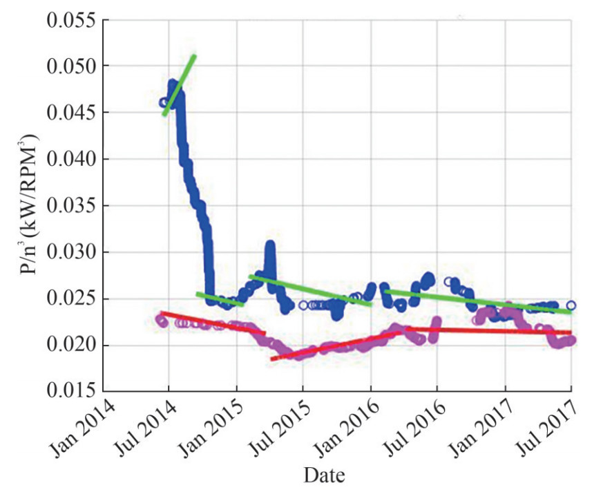Figure  7  KPIa for the two vessels (moving mean & trend)

Download: Full-Size Img

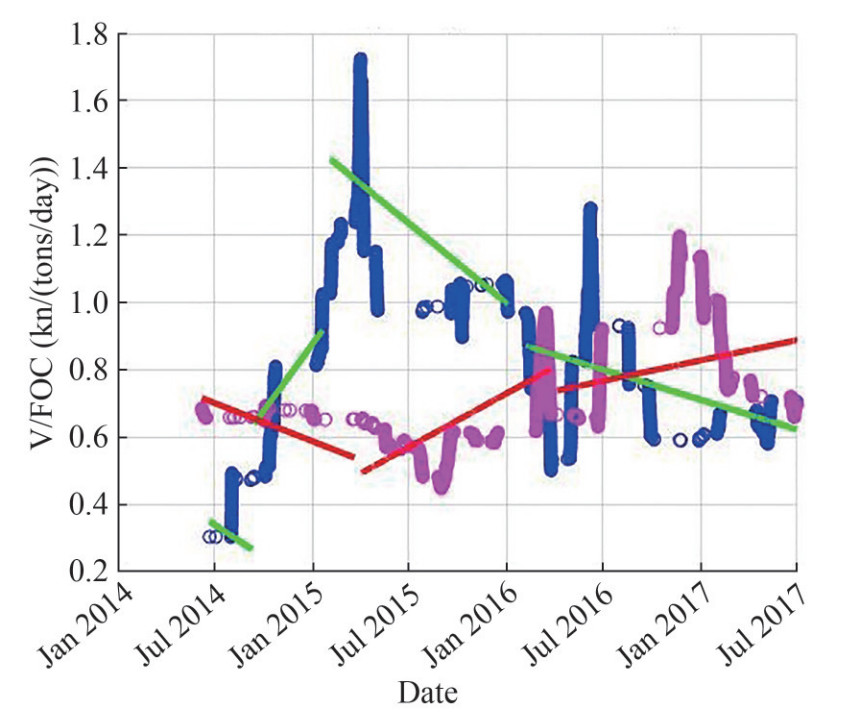Figure  8  KPIb for the two vessels corresponding the ballast loading condition (moving mean & trend).

Download: Full-Size Img

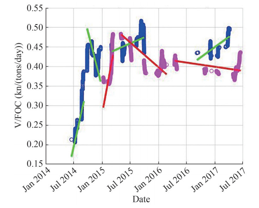Figure  9  KPIb for the two vessels corresponding the laden loading condition (moving mean & trend).

Download: Full-Size Img

3.2.1   Discussion on KPIa results

As shown in Figure 7, the initial difference between the two vessels' KPIa is significant. In the pre-dry-dock period (Periods 1A and 2A) Vessel 1 receives KPIa values of around 0.045 while Vessel 2 receives values that are almost half in size (about 0.023). In addition to that, Vessel 1's KPIa has an upward trend while Vessel 2's a downward one, a fact that causes even greater difference. Towards the end of Period 1A, the KPIa values of Vessel 1 are more than double those of Vessel 2. The gap between the two KPIa values depicts the significant difference in the performance levels of the two similar vessels and highlights the poor efficiency of Vessel 1.

Once Vessel 1 has its propeller polished, its KPIa reduces to nearly half its previous values (from 0.045 to 0.026), managing to cover the majority of difference with Vessel 2's KPIa. Apart from narrowing the difference, the propeller polishing seems to create ground for further improvement as Period 1B's trend line is almost parallel to that of Period 2A, indicating that the two KPIa decrease at similar rates. As a result, the performance gap between the two vessels is temporarily stabilized.

The two vessels initially react differently to the dry-dock repairs. Vessel 1's KPIa is increased from 0.026 to around 0.0275 (less than 10% increase) while Vessel 2's is significantly reduced (about 20%). However, this widening of the gap between the two KPIa has a short-term effect, as the trend line of Period 1C is downward while that of Period 2B upward. The contrast between the two trends reveals that while the performance of Vessel 2 is gradually deteriorating, a result that can be expected due to the increasing hull fouling, Vessel 1's performance is actually improved, despite the fouling. This contradictory pattern can be explained by the duct installation which manages to decrease KPIa for Vessel 1 in the long-term, when the effect of the hull cleaning repair is weakened.

During the second year after the dry-dock, Vessel 2's trend line seems to have stabilized at a value of 0.0215 while Vessel 1's continues to decrease, but at a lower rate. The decrease of Vessel 1's reduction rate is anticipated as the fouling is more severe. However, due to the increased performance achieved by the duct, the KPIa of Vessel 1 continues its slight decrease. As a result, the vessel's performance gap reaches an overall minimum at the end of the measuring period (0.0235 vs 0.0215).

The impact of the duct is revealed as time passes and the effect of the propeller polishing and hull cleaning are weakened. Even though it is the propeller polishing that manages to breach the initially huge gap, it is due to the duct that the main ground is maintained in the long-term and a further narrowing of the difference is achieved.

3.2.2   Discussion on KPIb results

Focusing initially on the ballast loading condition (Figure 8), Vessel 2's fuel efficiency is higher than Vessel 1's, reaching more than double KPIb Ballast values (0.72 vs 0.35). The trend lines of Periods 1A and 2A are both downward, with that latter having a smaller slope which indicates that the deterioration of performance, is slower for Vessel 2. As a consequence, towards the end of period 1A, the difference between the two KPIb Ballast is slightly increased (0.65 vs 0.27). By examining the laden loading condition (Figure 9), Vessel 1's KPIb Laden values are initially significantly low (around 0.17) while Vessel's 2 are higher (around 0.29), with Period 2A beginning after the end of Period 1B (propeller polishing). The initial low values are counterbalanced by the upward trends of the Period 1A's and Period 2A's trend line, which cause the KPIb Laden values to reach 0.31 and 0.43 respectively (80% increase vs 40% increase). The initial performance gap between the two is narrowed due to Vessel 1's higher increase rate (greater slope).

Once Vessel 1 has its propeller polished a significant alteration in performance is noticed. Vessel 1's KPIb Ballast values are instantly increased by about 150% (from 0.26 to 0.64) causing the Period 1B's trend line to surpass the Period 2A's one very quickly. In addition to that, the Vessel 1's trend line is steeply upward in contrast with the Period 2A's trend line which is downward. As a result, the performance gap between the two vessels is widened as time goes by, with Vessel 1's KPIb Ballast reaching a value of 0.92 while the respective value of Vessel 2 is less than 0.58. This significant alteration in Vessel 1's performance underlines the positive effect of the propeller polishing, which manages to increase fuel efficiency by a rate of about 150% in a small period of time. In the laden condition, Vessel 1's KPIb Laden is increased to 0.5 (about 60% increase), managing to surpass Vessel 2's values and significantly improving fuel efficiency. However, the effect of the propeller polishing is gradually weakened, and Period 1B's trend line is downward. As a result, at the end of the period, Vessel 1's KPIb Laden values are decreased by 30% (from 0.5 to 0.36), approaching the pre-polishing performance level. It can be understood that while the propeller polishing manages to instantly increase fuel efficiency, and thus performance, its effect is quickly reduced.

The two KPIb Ballast initially react differently to the dry-dock repairs (Figure 8). Vessel 1's KPIb Ballast is significantly increased from 0.92 to 1.43 (50% increase) while Vessel 2's decreases from 0.54 to 0.49 (about 10%). However, this widening of the gap between the two KPIbs has a short-term effect, as the trend line of Period 1C is downward while that of Period 2B upward. By the end of Period 1C, however, the gap remains significant (1.00 vs 0.73) as the vessels' initial reactions to the dry-dock have not been counterbalanced by the trends. The effect of the dry-dock seems to last longer for Vessel 2 than it does for Vessel 1, whose performance deteriorates towards the end of the first post-dry-dock year. In the laden condition (Figure 9), Vessel's 1 KPIb Laden is increased by about 20% (from 0.36 to 0.44) while Vessel 2's also increases but a slower rate (10% increase, from 0.43 to 0.48). Due to Period 1B's downward trend and Period 2A's upward, Period 2B's trend line manages to surpass Period 1C's for a small period of time. However, Vessel 1's trend line is slightly upward, achieving KPIb Laden values of around 0.475 (almost 10% increase) by the end of the first post-dry-dock year, while Vessel 2's trend line is downward and the respective KPIb Laden is reduced by about 20% in the first post dry-dock year (from 0.48 to 0.38).

During the second year after the dry-dock, in the ballast condition, Vessel 1's trend line continues its downward pattern, indicating that performance is reduced as the time passes, a phenomenon that is possibly explained by the constantly increasing hull fouling. On the other hand, Vessel 2's trend line, despite suffering an initial drop, continues its upward trend but at a lower slope, causing the KPIb Ballast values to increase at a lower rate. Eventually, Vessel's 2 trend line surpasses Vessel 1's and the performance gap between the two vessels continues to grow given their trends. Towards the end of the measuring period, the difference between the two KPIb Ballast is about 0.3 (0.62 vs 0.89) with Vessel 1's values returning to a similar level as the one achieved at the beginning of Period 1B (propeller polishing). As far as the laden condition is concerned, Vessel 2's KPIb Laden initially increases to 0.41 and continues its decline, but at a lower rate, reaching values around 0.39 at the end of the measuring period. On the other hand, Vessel 1's trend line is steeply upward and manages to counterbalance an initial 15% reduction of KPIb Laden values (from 0.475 to 0.415) reaching values around 0.48, greater than those achieved during the first post-dry-dock year.

Overall, despite Vessel 1's initial increased performance due to the propeller polishing and the dry-dock, Vessel 2 manages to reach higher KPIb Ballast values in the long-term. The effect of the duct is not depicted in the particular loading condition as the deterioration of Vessel 1's performance, due to the hull fouling and the weakening of the dry-dock effect, is not counterbalanced in the long run. In the laden condition, however, Vessel 1 manages to reach KPIb Laden values that approach the overall maximum achieved during the propeller polishing, towards the end of the measuring period, when the effect of the propeller polishing and the dry-dock is severely weakened if not complete eliminated. At the same time, Vessel 2's KPIb Laden follows a more anticipated pattern by initially increasing after dry-docking and eventually declining due to the weakening of the dry-dock's impact. The difference in the performance pattern of the two vessels can be explained by the propeller duct which successfully manages not only to preserve the KPIb Laden values achieved after dry-docking but also to increase them, counterbalancing the negative effect of hull fouling and achieving greater fuel efficiency in the long run.

4   Fuel oil consumption prediction-A multiple linear regression model

4.1   Introduction

A regression analysis is performed to produce a model that can predict the fuel oil consumption of the two vessels in the post dry-dock era, which is divided into two parts, one for the first post dry-dock year (DD1) and one for the second (DD2).

The FOC-EP relationship is linear and, thus, a linear regression model predicting the consumption given the shaft power is expected to produce solid results, as shown in Aldous (2015). However, this study aims to create a regression model to derive predictions for the fuel oil consumption through the utilization of other related variables such as the speed through water, the mean draft, the trim, the wind speed and the rudder angle. For the speed variable (STW), its square value is also examined along with the rest of the variables as it appears to better express the observed FOC-STW relationship.

The regression dataset is based on the dataset produced in the data processing section, while the data processing actions that used for the KPI's calculation are ignored. However, a filter concerning the speed through water is applied, omitting speed values less than 8 kn. This elimination of slow ship speeds, which account for a very limited portion of the dataset, causes an improvement of the regression models and leads to better predictions of the fuel consumption without defying the natural aspect of the problem since such vessels rarely travel in speeds under 8 kn.

A population model for a multiple linear regression (MLR) model that relates a y variable to a number p of x variables can be written as:

where:

· y_i : the i-th observation of the dependent variable.

· x_ij : the i-th observation of the j-th independent variable.

· β₀ : the regression intercept term.

· β_j : the slope coefficient of the j-th independent variable.

· ε_i : the error term of the i-th observation (normal distribution).

It can be understood that the model relies on the assumption that there is a linear relationship between the independent variable and the predictors. Each β coefficient represents the change in the mean response, E (y), per unit increase in the associated predictor variable when all the other predictors are held constant. The intercept term, β₀, represents the mean response, E (y), when all the predictors are zero.

The MLR model that makes predictions for the y variable can be written as:

where:

· $ \stackrel{\frown}{y_{i}}$ : the predicted/fitted value of the i-th observation of the dependent variable y.

· x_ij : the i-th observation of the j-th independent variable.

· b_j : the sample estimates of the β_j coefficients and are calculated as follows:

For each observation a residual (error) term is calculated:

4.2   Regression metrics

The regression analysis involves the calculation and interpretation of some statistical quantities that are briefly presented in Tables 7 and 8.

4.3   Correlations

As part of the regression model's preparation, the correlations among the examined variables (predictors) are calculated and presented in Tables 9 and 10. High correlation among the predictors may cause multicollinearity and as a result, models that use highly correlated predictors are avoided. Multicollinearity occurs when a predictor of the model can be linearly predicted from the other independent variables with a substantial degree of accuracy. The presence of collinearity causes the coefficients of the model to change erratically in response to small changes in the data. While the phenomenon does not reduce the reliability of the model and its predicting strength within the sample dataset, it may produce a regression model that gives invalid results about individual predictors and cannot distinguish which variables are redundant with respect to others. The effect of multicollinearity is measured by the Variance Inflation Factors (VIFs).

4.4   Best subsets

The best subsets analysis aims at identifying the most suitable regression model by comparing all the possible models, using a specified set of predictors. Despite the fact that the unique model that combines all the available variables is by definition the best in terms of R², models with fewer parameters may provide insignificantly smaller R². As a result, an efficient model with less variables is often chosen as it offers greater flexibility, reduces the possibility of multicollinearity and avoids overfitting that may occur at high R² values when the model is overly customized to fit the peculiarities of the random noise of the sample.

For different number of variables the best subset, in terms of R², is presented in Table 11, Table 12, Table 13 and Table 14.

It can be observed that Vessel 1's regression models have greater R² values than Vessel 2's which cannot surpass the 70% threshold that is easily achieved by almost all Vessel 1's models. As a result, Vessel's 1 dataset provides better FOC predictions than Vessel 2's.

Speed through water squared is the most important independent variable of the FOC regression models as it solely explains a lot of the variation of the predicted fuel oil consumption, something depicted by the big R² values of the single-variable models. While STW is an equally important parameter, it is not used in the chosen model in order to avoid multicollinearity.

The fuel oil consumption is correlated more with the mean draft (TM) than with the trim (TRIM). This relative advantage of TM is shown in the above models; when only one of two variables can be picked, mean draft is always preferred over trim. Taking the above into account along with the fact that mean draft and trim are highly correlated (multicollinearity), the chosen regression model shall contain the mean draft variable but not the trim one.

The addition of the wind speed variable (WS) significantly increases R² and reduces the C_p and S values for Vessel 1's models. As a result, WS is the second more significant variable and is chosen right after the speed variables. However, its impact is less significant on Vessel 2's models, for which the TM variable is more crucial. Overall, WS introduces the impact of the weather to the models and manages to improve their prediction without causing multicollinearity since it is not significantly correlated with any of the other predictors. As a result, it is chosen as a predictor of the regression.

The addition/subtraction of the rudder angle variable (RA) to/from a model has little impact on the calculated statistical quantities, a fact that clearly indicates its statistical insignificance to the regression analysis. This conclusion perfectly agrees with the low correlation between the RA and FOC variables. This effect has been strengthened due to the inclusion in the dataset of ship speed values above 8 kn.

The 3-variable model that is chosen (STW2-TM-WS) provides satisfactory R² values, compared with the maximum possible ones that are achieved by the 6-variable model, without including many predictors, a choice that may cause overfitting or lead to an unnecessarily complicated model. The model used by Safaei et al. (2019), utilizes the speed through water, the displacement and the wave height to predict the fuel oil consumption of 4 VLCCs, achieving high R² values. Similarly, the current model combines 3 physical quantities that characterize sailing conditions; the vessel's speed, its loading condition (expressed by the mean draft rather than the displacement) and the weather conditions (expressed by the wind speed). The chosen predictors are lowly correlated and, thus, the risk of multicollinearity is avoided.

4.5   Regression models

The basic characteristics of the four 3-variable regression models are presented in Table 15, Table 16, Table 17 and Table 18.

The constant term is in all cases negative, and its absolute value is reduced by almost 50% from Vessel 1's models to Vessel 2's. On the other hand, while a unit change of Vessel 2's mean draft causes about one-unit change of the fuel consumption, Vessel 1's TM has about half the impact of FOC. Finally, despite a slight gradual reduction of STW2 coefficients from the first case (Vessel 1-DD1) to the last (Vessel 2-DD2), all values are close to each other.

Despite the variations described above the most notable difference between the two vessels' model is the coefficients concerning wind speed. Vessel 1's models have positive WS coefficients (around 0.3) while Vessel 2's negative ones. This change of sign reflects both a physical phenomenon and a statistical one. It can be implied that throughout the measuring period, Vessel 2 experienced more journeys/travel hours of favorable winds that aided the vessel's navigation while Vessel 1 had fewer hours of fair winds. As a result, the increase of wind speed is a favorable phenomenon for Vessel 2's navigation as it reduces the amount of fuel needed to reach a certain speed, whereas such increase has a opposite effect on Vessel 1, forcing it to increase the fuel consumption in order to overcome the added wind resistance. Despite the possible validity of the above assumption, for its proper assessment an additional physical quantity is needed: the wind speed's (relative) direction. If the direction of the wind speed is to be provided, then a more proper evaluation of the above assumption can be conducted by introducing another predictor to the regression models and assessing its effect on the response variable. However, the data for the wind direction are not available for the examined vessels so such an assessment cannot be made. Instead, despite the sign contradiction, the discussed 3-variable model is used for both vessels in this preliminary regression analysis. Due to the larger amount of fitting of Vessel 1's models (higher R² values), it can be assumed that in a more complete and solid model, the WS coefficient would be positive.

Except for the above inconsistency, the chosen model has an adequate performance. The calculated Variance Inflation Factors of the selected predictors are low (just above 1), suggesting that there are no multicollinearity problems in the models as the independent variables are not significantly correlated.

The fitting of the models for the DD1 period is show in Figure 10 for both vessels.

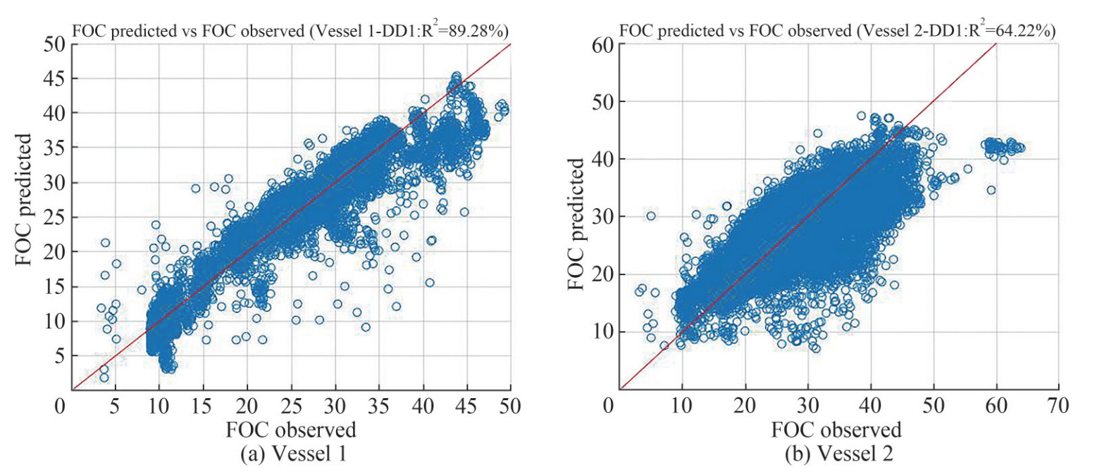Figure  10  Regression fitting for DD1

Download: Full-Size Img

4.6   Case study

For the selected 3-variable regression model, a case study is performed in order to evaluate and compare the FOC predictions between the two examined periods (DD1 & DD2) as well as between the two vessels (Vessel 1 & Vessel 2). Four different cases are examined with each case concerning a different wind speed and loading condition (expressed by the mean draft).

· Case 1: WS = 0 m/s & TM = T_ballast

· Case 2: WS = 0 m/s & TM = T_laden

· Case 3: WS = 10 m/s & TM = T_ballast

· Case 4: WS = 10 m/s & TM = T_laden

The first part of the case study is concerned with the comparison of fuel oil consumption values between the two examined periods (DD1 & DD2) for both vessels. Predictions are provided by the selected regression model whose predictors' values differ from case to case (WS & TM). Six different characteristic speeds through water are examined: STW = 10-15 kn. In addition, vessel 1 encountered wind speeds up to 10 m/s for the approximately 35% of its time duration while for vessel 2 the respective value is approximately 55%.

The second part of the case study is concerned the comparison of fuel oil consumption values between the two vessels (Vessel 1 & Vessel 2) for each examined period. In contrast with the previous part, the second part does not focus on a specific speed through water value. Instead, the FOC-STW curve of each vessel is produced by the respective regression model for Case 1 and Case 2. The vessels' curves are plotted in common in Figure 11 and compared over time (DD1 & DD2) for a range of STW values. Only Cases 1 and 2 are examined at the second part due to the contradiction between the WS coefficients' sign (positive for Vessel 1 and negative for Vessel 2). Therefore, a comparison involving the wind speed between the two vessels cannot be supported.

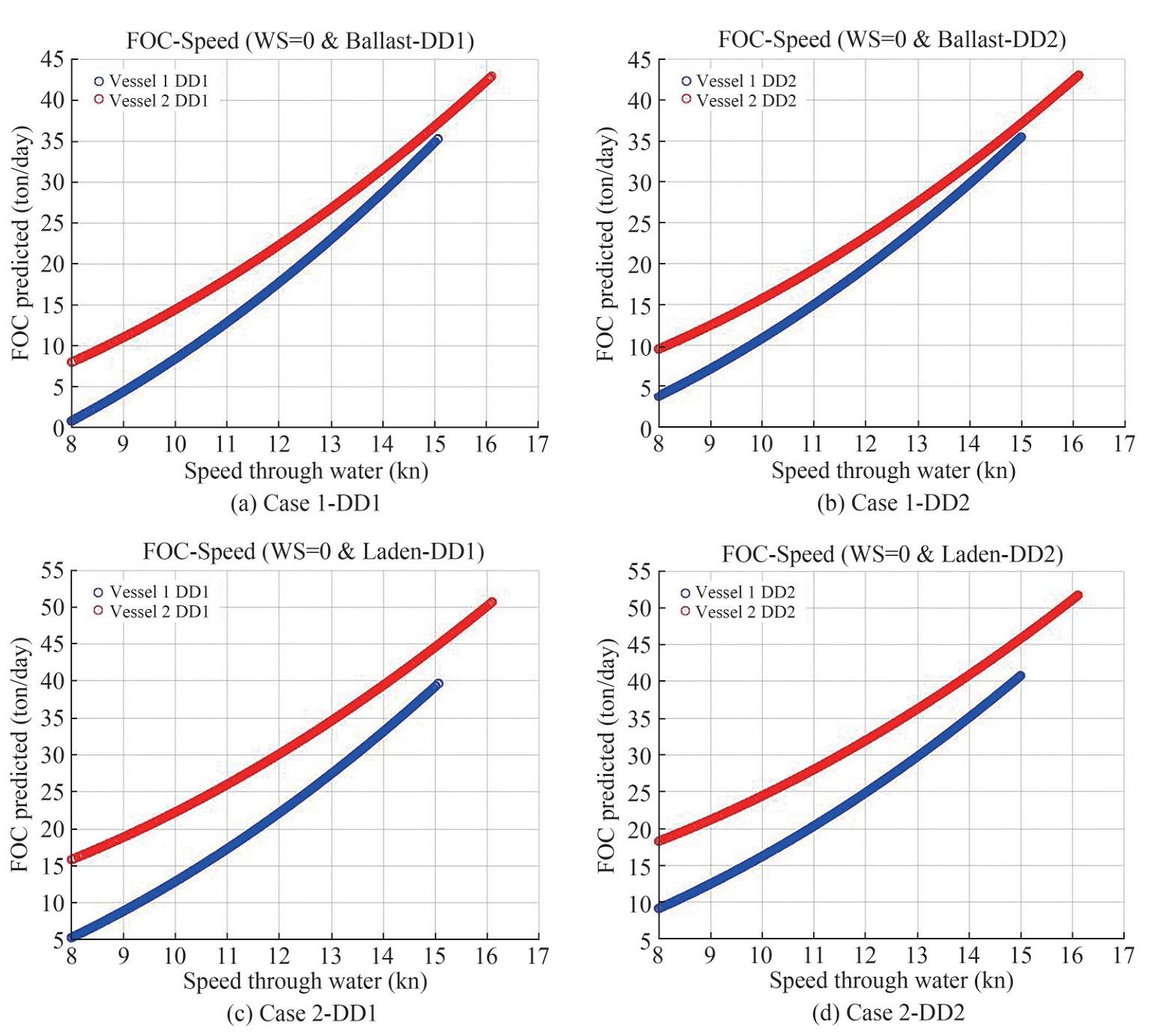Figure  11  FOC-STW

Download: Full-Size Img

4.6.1   Part A: DD1 vs DD2

The predicted FOC values are shown in Table 19, for Vessel 1, and in Table 20, for Vessel 2.

As it can be observed both Vessel 1 and Vessel 2 consume less fuel oil when travelling at lower speeds, a prediction that is in accordance with the real-time operation expectations. Furthermore, in each case, the predicted FOC is greater for DD2 than for DD1. However, the increase becomes significantly smaller as the speed rises, leading to insignificant differences (1-7%) for STW = 14-15 kn.

Through comparison of equal-draft cases for Vessel 1 it can be understood that while wind speed generally increases FOC (positive coefficient) it has no significant effect on the relative DD1 - DD2 differences, which mainly depend on STW and TM. Another observation is that greater drafts (laden condition) cause about a "+2%" increase in the aforementioned gap for all speed except the lowest one. Overall, while the duct's long-term effect is not depicted by the predicted FOC values, the stabilization of the values between DD1 and DD2, expressed by the percentage difference, for the high speeds indicates an increased performance that may be related to the Mewis duct. However, this is an assumption that cannot be positively verified due to the high level of uncertainty that lies within the 2-6% difference.

For Vessel 2, while the increase of draft leads to greater FOC values, wind speed has an opposite effect that is expressed by the negative coefficient of the WS variable. Wind speed seems to significantly increase the relative difference of FOC between DD1 and DD2 while TM has a more limited effect. The assumption made for Vessel 1 seems to be invalid if the patterns of Vessel 2 are taken into consideration; while the consumption is higher in the DD2 period, the relative difference is gradually reduced as speed is increased for both vessels. This similarity does not allow for the relative reduction to be attributed to the Mewis duct.

4.6.2   Part B: Vessel 1 vs Vessel 2

As shown in Figure 11, for both cases, Vessel 1 is predicted to consume less fuel oil than Vessel 2 for both periods. The difference in FOC between the vessels is greater for lower speeds and reduces as speed increases, reaching a minimum at 15 kn. Both vessels' FOC values increase during DD2, however, Vessel 2's increase is smaller, causing the difference between the fuel consumption of the vessels to drop during the second post dry-dock year. For Case 2 consumptions are generally greater, a fact that is expected due to the added cargo weight. The difference in consumption between the two vessels is greater than the one in the ballast condition, underlining Vessel 1's added performance advantage in increased drafts which can be attributed to the Mewis duct.

5   Conclusions

The paper attempts to evaluate the energy savings of an energy-saving device, the Mewis propeller duct, through the utilization of a practical performance monitoring framework. Two sister vessels are monitored for a three-year period, during which one had a Mewis duct installed. The key idea was to assess the duct's effect by performing a comparison between the pre-duct and the post-duct era as well as between the two sister vessels for the same period. The study approaches the problem via two routes; a Key Performance Indicators (KPI) analysis and a MLR model.

The first part of the paper was devoted to the preparation of the database to be utilised by both methods. Such a pre-processing step aims at detecting outliers and eliminate them without discarding desirable data that provide valuable information. Moreover, the data filtering process targeted the identification of time periods corresponding to sea-travel passages, as well as of no significant effect of weather conditions and the ruder operation, to limit the analysis within conditions allowing the assessment of the propulsive efficiency. This procedure, while belonging to the initial steps of performance monitoring evaluation methods, should be considered of vital importance as it is measurements and the true physical relationships among the quantities. The analysis with the KPIa revealed that Vessel 1 significantly improved its performance when her propeller polished and approach the performance of Vessel 2. This propeller's polishing is indeed a popular industry measure to improve propulsive efficiency. After the occurrence of dry-dock, Vessel 2 experienced a performance increase for almost 1 year period, while for the remaining time was remained approximately constant. However, in the long-term the effect of the Mewis duct on Vessel 1 was identified. Specifically, when the effects of propeller polishing and hull cleaning fade in time, Vessel 1 shows an improving performance trend that is attributed to the only event with long-term impacts, the Mewis duct fitting. On the other hand, the analysis with KPIb resulted in similar findings for the laden condition, where after dry-dock Vessel 2 experiences a steady deteriorating performance, whereas Vessel 1 shows on the contrary an improvement. The examination for the ballast condition did not reveal any significant improvement due to the Mewis duct. As a result, it can be deduced that in greater drafts, which occur for loaded ships, the effect of the Mewis duct is enhanced.

As mentioned earlier, the second approach to the problem was through the development of MLR models utilizing operational data after the drydock periods and again proceeding with a relative comparison among the two vessels. After a best subset analysis and based on the findings of Part B and specifically the derived FOC-STW curves, it is resulted that for lower ship's speed range and for the laden condition the effect of the Mewis duct is more pronounced as Vessel 1 consumed less fuel than Vessel 2 for both periods (DD1 and DD2) and assuming no-wind effect. Finally, the effect of the weather conditions on the efficiency of such an energy saving device was considered a more complex problem to be examined. Given the fact that no wave data were available, the wind speed values kept for analysis correspond to weather conditions of low severity limiting the outcomes only to such conditions. However, by not including time instances with excessive ship motions or significant added resistance values, the analysis avoids involving complex interactions and effects on the system.