Nomenclature

1   Introduction

Due to the advantages of high safety, high efficiency and low cost, pipelines are widely applied in the transportation of large quantities of oil and gas over long distances (Xie and Tian, 2018). However, pipelines also face big challenges with the exploitation of oil and gas into deep and/or ultra-deep water (Cai et al., 2017; Chin et al., 2020). One of the biggest challenges is the corrosion defect, which may significantly compromise structural integrity and thereby bring severe consequences to the safety of structures and environment (Macdonald and Cosham, 2005; Mohd et al., 2015; Cai et al., 2018b, 2019). Therefore, it is necessary to find effective ways to evaluate the integrity of the pipeline so that the risk of pipe leaking or rupture may be reduced.

There have been large interests in the effect of corrosion defects on line pipes subjected to internal pressure since the late 1960s (ASME B31G, 2012). Researchers are trying to find an exact relation between corrosion defects and internal pressures. Thus, a large number of experiments on the burst pressure of corroded pipelines were conducted. Cronin et al. (1996) evaluated assessment procedures of pipeline corrosion defects from pipe experiments. Benjamin et al. (2000) carried out a burst test (9 specimens together) to investigate the behavior of a pipeline with long corrosion defects. Choi et al. (2003) proposed limit load solutions for corroded pipelines of API 5L X65 material (Specification, 2004) through burst tests with machined pits. Astanin et al. (2009) conducted a pipe test to verify an empirical method for the burst pressure of corroded pipelines. Cai et al.(2018b, 2019, 2018a) studied the effect of a single corrosion defect on pipe strength based on both experimental tests and numerical simulations.

As a result, a considerable number of empirical and semiempirical formulas (Cai et al., 2018b; ASME B31G, 2012; DNV, 2017; Chen et al., 2015b; Amaya-Gómez et al., 2019) are well-established. Choi et al. (2003) proposed a simple formula for the burst prediction of X65 pipelines assuming that the pipe burst strength only relies on factors such as diameter to thickness ratio (D/t), corrosion depth to thickness ratio (d_n/t) and the normalized corrosion length (l_n/ $\sqrt {Rt} $). Chen et al. (2015a) proposed a formula for the burst prediction of X80 and X90 pipelines through a small-size dataset. An extra parameter about the corrosion width to diameter (w_n/D) has been considered. Cai et al. (2018b) constructed a similar formula for corroded pipelines under bending moments based on physical models and experimental data. The benefit of such empirical formulas is obvious, for instance, a rapid evaluation of corroded pipes by hands.

Recently, the low price environment of oil and gas motivates industry to extend the useful productive life of corroded pipelines (Rosen et al., 2016). Therefore, improved models and alternative methods for the prediction of residual burst strength of pipes are needed. The past few years have witnessed the booming of artificial intelligence (Xie and Tian, 2018; Bishop, 2006; LeCun et al., 2015). The successful applications of machine learning in different fields are revolutionary (Ghaboussi and Sidarta, 1998; Ling and Templeton, 2015; Fukami et al., 2020; Rafiei and Adeli, 2017; Sen et al., 2019; De Masi et al., 2015; Gholami et al., 2020; Cai et al., 2021). Tremendous improvements in terms of training efficiency, learning accuracy and model performance are made thanks to the increase of computational capacity (LeCun et al., 2015). In the field of pipeline, De Masi et al. (2015) proposed a neural network model to assess the corrosion of subsea pipelines in terms of corrosion rate, metal loss, the area of loss and the corrosion numbers. Ossai (2020) built a corrosion growth model based on the historical operation parameters through a feedforward multilayer neural network. Abbas and Shafiee (2020) discussed the prediction method by using artificial intelligence for corrosion models. Chin et al. (2020) initially studied the burst pressure of corroded pipes based on a two-layer neural network. Gholami et al. (2020) predicted the burst pressure of high-strength carbon steel pipelines with gouge flaws using artificial neural network based on a dataset from finite-element analysis. Amaya-Gómez et al. (2016) generated equivalent dimensions of grouped corrosion defects accounting for defect interactions, using the SVM and K-mean methods. Liu et al. (2019) adopted supervised machine leaning algorithms such as SVM and Random Forest to match corrosion features. Mattioli et al. (2019) stated that building pipeline digital twins with machine learning algorithms is necessary for the future safety of pipeline operations.

However, the application range of existing empirical models are limited, and the performance is not high due to a lack of generalization ability. For instance, a fitted model for pipelines with X65 material and a random shape corrosion can be hardly applied to X80 pipelines with a rectangular shape corrosion. In a foreseeable future of digitalization for pipeline service, such empirical formulas from traditional methods may not serve this purpose well. Alternatively, the finite-element method based on traditional physical mechanism is normally adopted for prediction, but it is too time-consuming. Therefore, the objective of this paper is to explore a novel data-driven methodology for the prediction of the burst strength of corroded pipelines without too much domain knowledge needed, which can overcome such drawbacks. In this research, only an external corrosion defect is considered. The supervised machine learning algorithms, including ANN, SVM and LR, are deployed. All the data are found from literature and are properly arranged for utilisation. Note that one big problem for data-driven methods is the limited size of dataset in pipeline engineering, which affects the generalization ability of proposed models. In other words, the proposed models may still not be accurately used for unseen case predictions, which is an unavoidable drawback and will introduce bias. Thanks to the transfer learning (Weiss et al., 2016), which is able to account for previous learned knowledge, the latest development and the successful results in the field of artificial intelligence are made. Thus, the current research work is meaningful and can be further served as surrogate models by transfer learning. Further work on the application of transfer learning on pipelines will be done based on the results of current research.

The structure of this paper is arranged as follows. In Section 2, we introduce the internal mechanism of different data-driven algorithms. How to properly evaluate the trained models is described as well. In Section 3, the existing experimental data of corroded pipes found from literature are described. The characteristics of pipe corrosion and pipe experiments are illustrated. In Section 4, empirical formulas for corroded pipelines from DNV and ASME B31G are discussed. Afterwards, pipe data exploration is conducted in Section 5 so as to properly choose pipe features for model training. In Section 6, prediction models are proposed through typical machine learning algorithms and comparison results are discussed. Possible intelligent application of the improved models in digital operation/ monitoring of pipelines is analysed. Conclusions are drawn in Section 7.

2   Data-driven methodologies

Data-driven methodologies in terms of machine learning algorithms are generally used to construct prediction models. The typical algorithms, including ANN, SVM and LR, are deployed. These three models are chosen because of the popularity and widely used for regression problems in machine learning. Their strengths and weaknesses are introduced for a better application in practice. Evaluation strategies and how to improve trained models are discussed in order to obtain better performance.

2.1   Artificial neural network

ANN belongs to the category of DL (deep learning). Its successful application in practical engineering field has been revolutionary over the past years, which is motivated by the structure of biological neural circuits of human brains. This concept is commonly referred to MNN (multi-layer neural network), MLP (multi-layer perceptron) or DNN (deep neural network). ANN is constructed through connecting of perceptrons in layers. As can be seen in Figure 1, a perceptron (Rumelhart et al., 1986) is defined as the minimum unit of an entire neural network. Each perceptron is made up of many neurons, receiving and activating signal among different neurons. The weaknesses of applying ANN include complex training models, careful preprocessing of data and low-efficiency of training, whereas the strengths are high accuracy under limited dataset and demonstrated successful application in various engineering fields.

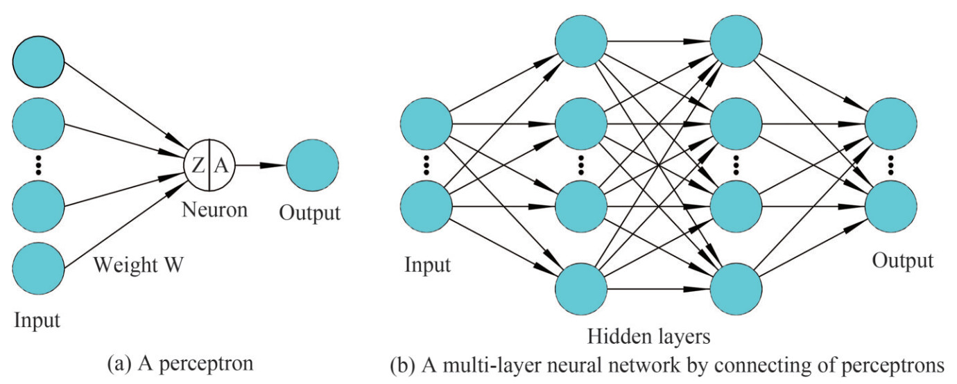Figure  1  Basic architectures of neural networks

Download: Full-Size Img

Given a set of training data X and labelled target y: X∈ R^{(n_x, m)}, y∈ R^{(m, n_y)}, the output prediction (ŷ) can be trained into a L-layer neural network based on their inner relation. In ANN, the values of units (Z) and their activation values (A) are computed based on a feed-FP (forward propagation), as expressed by Eq.(1). The W is the training weight and the b is the training bias. The superscript l denotes the layers of neural network (excluding the input layer, which is considered as the layer zero).

Note that the using of an activation function in hidden layers of neural network is crucial, which brings nonlinear effects for model training. Otherwise, the architecture of deep learning would be meaningless, making no difference with training by algorithms like linear regression. As seen in Figure 2, three basic types of activation functions are adopted in ANN (Haykin, 2007), including Sigmoid (g (Z)=(1+e^−Z)−1), ReLU (Rectified Linear Unit, g(Z)=max(0, Z)), and Tanh (hyperbolic tangent, g(Z)=(e^Z−e^−Z)(e^Z+e^−Z)⁻¹). e is the Euler's number. In general, the ReLU works better than the Sigmoid function for deep neural network (Nair and Hinton, 2010). However, it sometimes produces poor performance due to the discontinuous derivatives (Haghighat et al., 2020). The Tanh activation function can be then used accordingly. In this paper, only ReLU function is adopted in pipeline models.

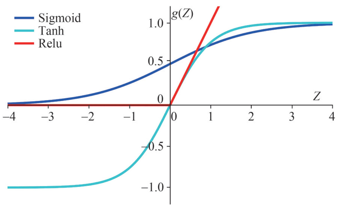Figure  2  Three typical activation functions (Haykin, 2007) including ReLU, Tanh, and Sigmoid

Download: Full-Size Img

In order to evaluate the trained model with respect to target (burst pressure in this paper), a loss function (J) is customized for objective optimization, as seen in Eq. (2). The BP (backward propagation) (Nair and Hinton, 2010) is deployed to calculate the derivatives in Eq. (3). The process procedure is denoted in Eq. (4), which provides detailed expressions of all necessary derivatives. In order to break the symmetry of neural network architecture during training, the Xavier initialization (Glorot and Bengio, 2010) strategy is deployed.

Figure 3 illustrates an example of a three-layers neural network in a pipeline model with two hidden layers and one output layer. The computation procedure of a neural network with FP and BP is explicitly explained for each layer. The ReLU function is used for the activation of hidden layers. Note that, in the output layer, there is no need to do an extra activation any more for regression problems since we only have one target (burst pressure).

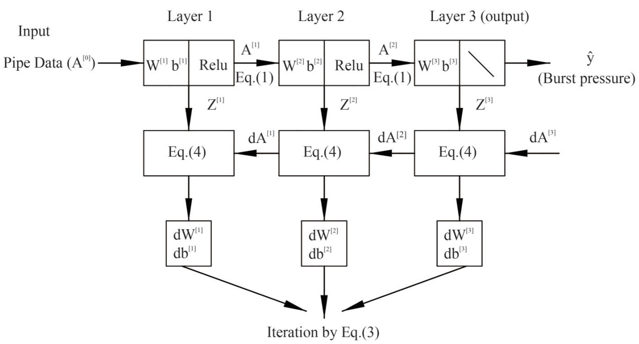Figure  3  Flowchart of the basic computation procedure of ANN using FP and BP for the training of pipe burst strength

Download: Full-Size Img

2.2   Support vector regression

SVM is considered to be one of the most powerful "black box" learning algorithms in conventional ML field (Bennett and Mangasarian, 1992; Cortes and Vapnik, 1995). By utilizing a cleverly-chosen optimization objective, it's one of the most widely used machine learning methods nowadays (Fukami et al., 2020; Smola and Schölkopf, 2004). The algorithm works well with sparse data but may provide a lower generalization performance for low-dimensional data. SVR (Support Vector Regression) is an extension of SVM for regression problems with the same internal mechanism (Bishop, 2006). The mathematical theory of SVM is first described, which will be used for the training of pipe models in Section 6.

In order to demonstrate how SVM works, a linear binary classification problem is considered here. As seen in Figure 4 (a), it illustrates a training set with two classes, indicated by circles and crosses. The target of this problem is to find a boundary line (or a hyperplane for high dimensional problems) to properly separate all samples. The decision boundary should be evenly distributed between the two classes of data with the maximum margin, expressed as F(X)=W^TX+b. Likewise, the learning process is to establish the function F(X) between input data and output target through mapping the training data into a high-dimensional feature space. The margin is defined as the distance between the decision boundary and the closest samples, expressed as (W^Tx_i+b)/‖W‖ based on the distance formula from a point to a plane in the Euclidean space. All the x_i are called support vectors which are samples to determine margins. Note that the numerator (W^Tx_i+b) is always a constant which does not affect optimization results. Hence, a constant value of 1 could be used for simplification in the distance formula.

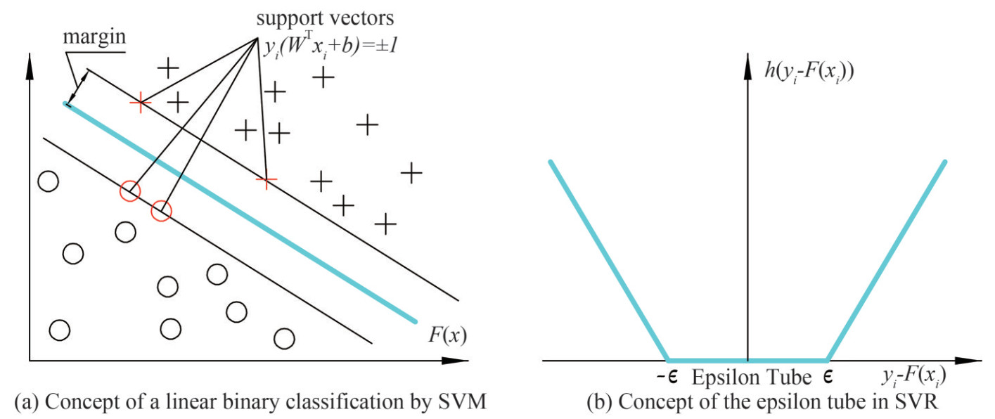Figure  4  SVM illustration

Download: Full-Size Img

Therefore, the task is to learn the best W and b in a decision boundary so that the margin in Figure 4 (a) is maximum when subject to y_i(W^TX_i+b)≥margin, ∀i, as shown in Eq. (5). X_i here indicates the matrix of training sample i, y_i is the signed values of +1 or − 1, representing different classes. Due to a reciprocal relationship, such optimization problem is further simplified as a minimum problem when subject to y_i(W^TX_i+b)≥1, ∀i, as seen in Eq. (6). The concept of soft margin (Bennett and Mangasarian, 1992; Cortes and Vapnik, 1995) is used so that an extra term is added into the objective function of Eq. (6) for penalty, as shown in Eq. (7).

As an extension of the SVM algorithm, SVR has been introduced to handle the regression problems. Instead of predicting the category label of an input as the SVM does, SVR is used to predict some discrete values. Following the same idea of the SVM, SVR introduces an ε-insensitive region around the function, called the ε-tube. Then, the regression problem is reformulated to find such ε-tube that it best approximates the continuous-valued function. More specifically, SVR first defines a convex ε-insensitive loss function (subject to the constraint h(y_i−W^Tf(x_i))=max (0, |y_i−W^Tf(x_i)|−ε)) to be minimized and then searches for the flattest tube that contains most of the training instances, as shown in Figure 4 (b). The f(x) is the mapping function, h() is the ε-insensitive hypothesis function (or extra loss) of predicted values and true values. Similar to the SVM, SVR can be used to regress a non-linear function, or a curve, through the use of kernel functions, the so-called "kernel trick" (Boser et al., 1992). Three kernels are used for the pipe model training in Section 6, including Linear, RBF, and Polynomial. SVR has great generalization capability and excellent prediction accuracy (Awad and Khanna, 2015).

2.3   Linear regression

In statistics (Downey, 2011), linear regression is a linear approach to describe the relationship between one set of variables (or target) and one or more explanatory variables (or features). As seen in Eq. (8), it indicates a linear relationship between true value y and feature x_i, where $\epsilon$ is the residual, w₀...w_n are the weights of features. The objective function is, therefore, to minimize the loss function (MSE (mean square error)) in the form of the least squares so as to find the best weight W and bias b, as seen in Eq. (9). One of the biggest weaknesses to apply regression is that a strong assumption is needed in advance based on data structure and physical theory, largely reducing the training accuracy. For instance, the corrosion width along pipe length is often assumed to have little effect on burst strength. The major factors, including corrosion size and material roughness, determine the resistance to material fracture failure and thereby the bust strength of pipes. With the increase of feature numbers, it is getting harder and harder to construct a model in advance with reasonable assumptions. Note that non-linear approaches (e.g., polynomial regression) can be also used for the fitting of models. However, more features are needed when no reasonable assumptions can be made. As a consequence, more data are needed for better accuracy, which is not practical to use in this paper. Therefore, only the linear regression models by using least-squares approach are adopted.

In order to avoid overfitting, regularization penalty should be introduced with extra penality. For the linear regression with the penalized version of least-squares (L²-norm penalty), it is called Ridge regression (Hoerl and Kennard, 1970), as seen in Eq. (10). With the increase of tuning parameter λ, the overfitting of model decreases. When using the Ridge algorithm, λ is not sensitive and may be set to large value between 1 and 100. For Lasso regression (Tibshirani, 1996), it uses the L¹-norm penalty, as seen in Eq. (11). With L¹ penalty, the weight in W is possible set to be zero. Hence, Lasso takes care of model selection by removing the least influential features. The λ in Lasso is sensitive so that it normally set to be small, ranging between 0 and 1. Besides, the ElasticNet algorithm (Zou and Hastie, 2005) is used, which is a convex combination of the Ridge and the Lasso. It can reduce the error over Lasso method.

2.4   Evaluation and improvement strategies

The training models by supervised machine learning algorithms generally face the bias-variance trade-off (De Masi et al., 2015; Haykin, 2007). The definition of variance is the variability of model prediction for a given dataset, indicating the spreading of data. Bias is the difference between the predictions of trained models and the true values. In general, models with high variance pay much attention to training data. The generalization ability on the test/ validation data which it has not seen before is not sufficient. In other words, such models may perform very well on a training set but have high errors on a test set (overfitting). For models with high bias, instead, little attention to the training set is paid. High errors occur on both training set and test/validation set. As a result, high bias causes the miss of relevant relations between features and target outputs, which is called underfitting. This evaluation criterion will be utilized for discussions among the trained pipe models in Section 6.

For regression problems, the coefficient of determination (R²) (Tabachnick et al., 2007) is used for the evaluation of model accuracy, expressed as R²= 1-SS_reg/SS_total. The ratio of the sum squared regression error (SS_reg) against the sum squared total error (SS_total) tells us how much of the total error remains in trained models. As a result, a R² of 1.0 indicates no error in the model, while a R² of 0 means that the model is no better than taking the mean value of data. A negative R² is also possible, indicating that the SS_reg is greater than SS_total and the prediction performance is even worse than using the mean value. The MSE can also be used as an indication of model accuracy.

In order to improve prediction models, strategies such as ensemble strategy (Naftaly et al., 1997) and transfer learning (Taylor and Stone, 2009) can be used. The ensemble strategy is to combine several improved models together so as to produce a better prediction performance. The framework of transfer learning will accelerate the convergence of machine learning using the current models as surrogate models, especially for problems with large-size dataset. The utilization of transfer learning is crucial in engineering fields where new samples are constantly added into.

3   Experiments data of corroded pipes

The pipeline corrosion is a natural process that happens when pipe materials interact with the working environment such as water and carbon dioxide. In this section, typical experimental tests of pipe burst strength are introduced. The definitions of corrosion characteristics in terms of shape, orientation and fabrication workmanship are given. Recorded pipe data from tests are categorized and discussed.

Figure 5 shows a typical failure mode of corroded pipes in experiments (Astanin et al., 2009). The failure in terms of a crack-like rupture occurs along the pipe longitudinal direction in the corroded region. This is due to the plastic collapse that occurred locally in the corrosion ligament when the von Mises stress exceeds the ultimate tensile strength of the material through this region. For pipelines without significant defects, plastic collapse may occur by a global geometric instability of the specimen. As a result of the decreasing wall thickness and the increasing of pipe ovalization, the structure suffers an increasing of stress (Cai et al., 2017). For pipe test in laboratories, the length of each specimen is varied, generally ranging between 1.0 m to 2.3 m as observed from existing data. The specimens ends are sealed with very thick steel plate so that the boundary effects could be eliminated. Nozzles are deployed on end plates which are used for pressure pumping.

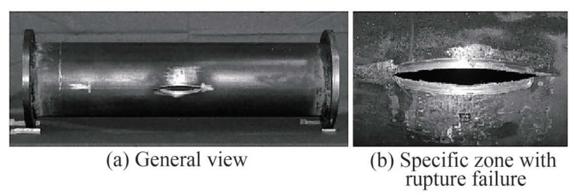Figure  5  The failure mode of the burst experiment of a corroded pipe specimen from Astanin et al. (2009)

Download: Full-Size Img

Corrosion defects are usually fabricated by two ways in a pipe test. One way is the machining method (such as spark erosion (Freire et al., 2006)), the other way is purely natural processes. Figure 6 shows the definition of corrosion geometry. The maximum corrosion depth through a real nature process is simplified as the depth of defect (d_n), while the maximum length of corrosion is simplified as the length of defect (l_n). The corrosion angle (θ_n) is defined as the angle between the pipe longitudinal axis and the corrosion length, ranging from 0° to 90°. For θ_n in 0 deg, the defect is considered as longitudinal corrosion, while for θ in 90 deg, the defect is considered as hoop corrosion. For other angles between 0 deg and 90 deg, the defects are all defined as angled corrosion in this study. Multiple corrosions normally appear on the pipe surface. Under this circumstance, scanning is conducted and then combining them into one patch automatically with software unless the corrosions are separated by a distance greater than six time of full pipe thickness as described by Cronin and Pick (2000). L₁ and L₂ in Figure 6 are parameters that would be only used for the burst pressure estimation by DNV-RP-F101 (DNV, 2017) in Section 4.

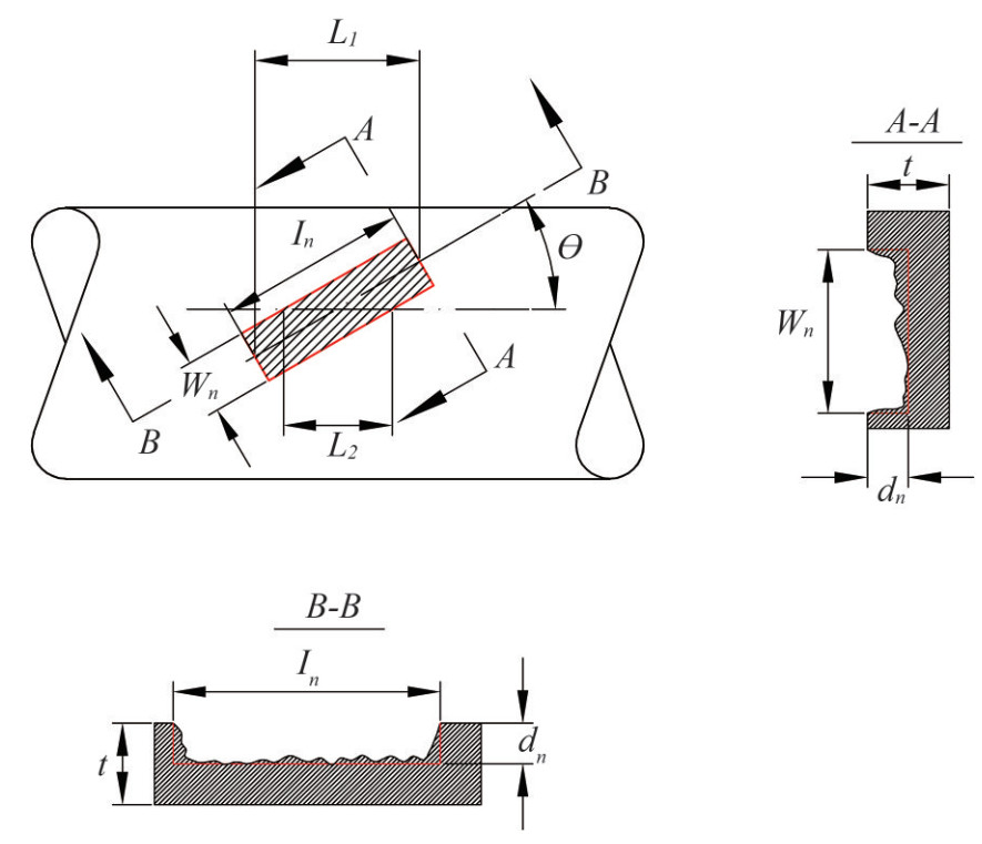Figure  6  Geometry of the simplified corrosion defect in the shape of rectangular profile in rotational angle (θ) in this paper

Download: Full-Size Img

Tables 1 and 2 present the two types of features recorded in a pipe burst experiment including numeric feature and categorical feature from literature (Cronin et al., 1996; Benjamin et al., 2000; Choi et al., 2003; Mok et al., 1991; Freire et al., 2006; Cronin and Pick, 2000). Not all original data and their features are listed here for the sake of clarity. Overall, 115 tests are obtained. Nine different line pipe materials are adopted based on API 5L (Specification, 2004), including the grades of A25, B, X42, X46, X52, X56, X60, X65, and X80. The numeric feature consists of the geometry of specimens, the geometry of corrosion defects and the material properties of specimen. Based on physical theory, failure stress is normally expressed as the function of such numeric features. Besides, the categorical feature includes corrosion shape, orientation, fabrication method, location, the grade of material and pipe type. For the corrosion shape which is not rectangular, it is defined as "Irregular". Only two types of corrosion defect method are defined: "Machined" and "Nature". Properly selection and investigation of all these pipeline features are very important in developing a reliable, riskfree and cost-effective prediction method, which will be discussed in Section 5.

4   Corrosion assessment in engineering standards

In this section, the estimation methods from engineering standards (DNVGL-RP-F101 (DNV, 2017), ASME B31G (ASME B31G, 1991) and the Modified B31G (ASME B31G, 2012)) for corroded pipelines are introduced. Note that there are some limitations of using these empirical formulas. For instance, ASME B31G does not apply to the crack-like corrosion defects or mechanical surface damage with a coarse surface. The corrosion damage should be located at the pipe center, not affecting by the pipe seams or girth welds. These limitations may introduce possible discrepancies of the prediction in Section 6.

4.1   Barlow's formula for intact pipes

Barlow's formula is widely used in the piping industry to compute the burst pressure (Pf) of intact pipelines without corrosion subjected to internal pressure, as seen in Eq. (12).

4.2   Empirical formulas in DNV

In DNVGL-RP-F101 (DNV, 2017), the formula for the failure pressure of pipes with a single rectangular longitudinally oriented defect subjected to internal pressure is proposed based on a large number of FE analyses, as seen in Eq. (13). The formulas may be applied to pipes with diameters ranging from 291.1 mm to 914.4 mm and the grades of pipeline material ranging from API 5L X42 to X65. For pipes with grades up to X80, however, these formulas may not be used due to model limitation. Note that the formula cannot be applied to corrosion shapes other than a single rectangular shape in pipe longitudinal direction. The measured defect depths should be less than 85% of the wall thickness.

where:

4.3   Empirical formulas in ASME B31G

Empirical formulas are also proposed in ASME B31G standard and its further modified version. The P_f of line pipes with medium strength and high material toughness can be expressed as Eqs. (15) and (16). The corrosion features in terms of longitudinal length (l_n) and depth (d_n) are accounted for. Note that when the rotational angle is less than 45 deg, as seen in Figure 6, the corresponding corrosion length (l_n) is changed to L₁ for calculation, otherwise, the most severe longitudinal section (L₂) should be considered. As we have noticed, an extra relation $l_{n}=\sqrt{20 D t}$ is roughly deployed to imply the severity of corrosion. M is the bulging stress magnification factor, as seen in Eq. (17). For plain carbon steel operated at temperatures below 120 ℃, the flow stress (P_flow) may be defined as Eq. (18).

For $l_{n}<=\sqrt{20 D t}$,

For $l_{n}>\sqrt{20 D t}$,

where:

In the modified ASME B31G (Kiefner and Vieth, 1989; Kiefiier and Vieth, 1990), the roughly relationship used to indicate the severity of corrosion is updated, expressed as $l_{n}=\sqrt{50 D t}$. The P_f is shown in Eq. (19). Different bulging stress magnification factor M is adopted within different corrosion severity regions.

For $l_{n}<=\sqrt{50 D t}$,

For $l_{n}>\sqrt{50 D t}$,

5   Data exploration for model training

In this section, the pipe experimental data described in Section 3 are statistically analyzed. All the data are split, cleaned and aggregated after careful investigation so as to choose proper pipe features for model training. A crossvalidation generator (Bishop, 2006) is used to randomly shuffle the pipe data, and to split the data into independent subsets for model training. Thus, the data are categorized into three different sets, including a training set (80% of all data), a validation set (10% of all data) and an extra test set (10% of all data). Note that, due to the limited size of dataset, only training dataset and validation dataset will be used for model performance evaluations in Section 6 to avoid bias. The accuracy from test dataset will be still presented as a reference.

5.1   Data exploration for the training by ANN

Data exploration is essential for the proper training of a machine learning model. As seen in Tables 1 and 2, the numeric features, such as pipe thickness and pipe outer diameter, can be directly applied on training after data cleaning. However, the categorical features such as pipe material grade need to be transformed before applying. Strategies including label encoding and one-hot encoding (Bishop, 2006) are used for the categorical features processing.

Feature importance should be determined so that we can properly keep and/or discard existing features for models. One of the strategies is to check the correlation coefficients between independent variables and the output target (pipe burst pressure (P_f)). It is defined as the covariance of two variables divided by the product of their standard deviations. The highly correlated features should be first selected. As seen from the heatmap in Figure 7, all the correlations among features are visualized. The legend of color denotes the level of correlation. The value close to 1 implies a strong positive correlation between two features, while the value close to −1 implies a strong negative correlation. The value of 0 indicates no correlation relation. We found that the parameters such as corrosion length (l_n), corrosion depth (d_n) and pipe outer diameter (D) have a large negative correlation to the burst pressure, while the pipe thickness has a large positive correlation to the burst pressure. The specimen length (L_p) and the corrosion width (w_n) have a very small correlation value to the burst pressure. These findings coincide with the former assumptions about the insignificant effect of corrosion width on the burst pressure of pipelines (Cai et al., 2018b; Choi et al., 2003). Therefore, these two features (L_p and w_n) are intentionally removed, and are not used for model training in Section 6 due to the limitation of data size.

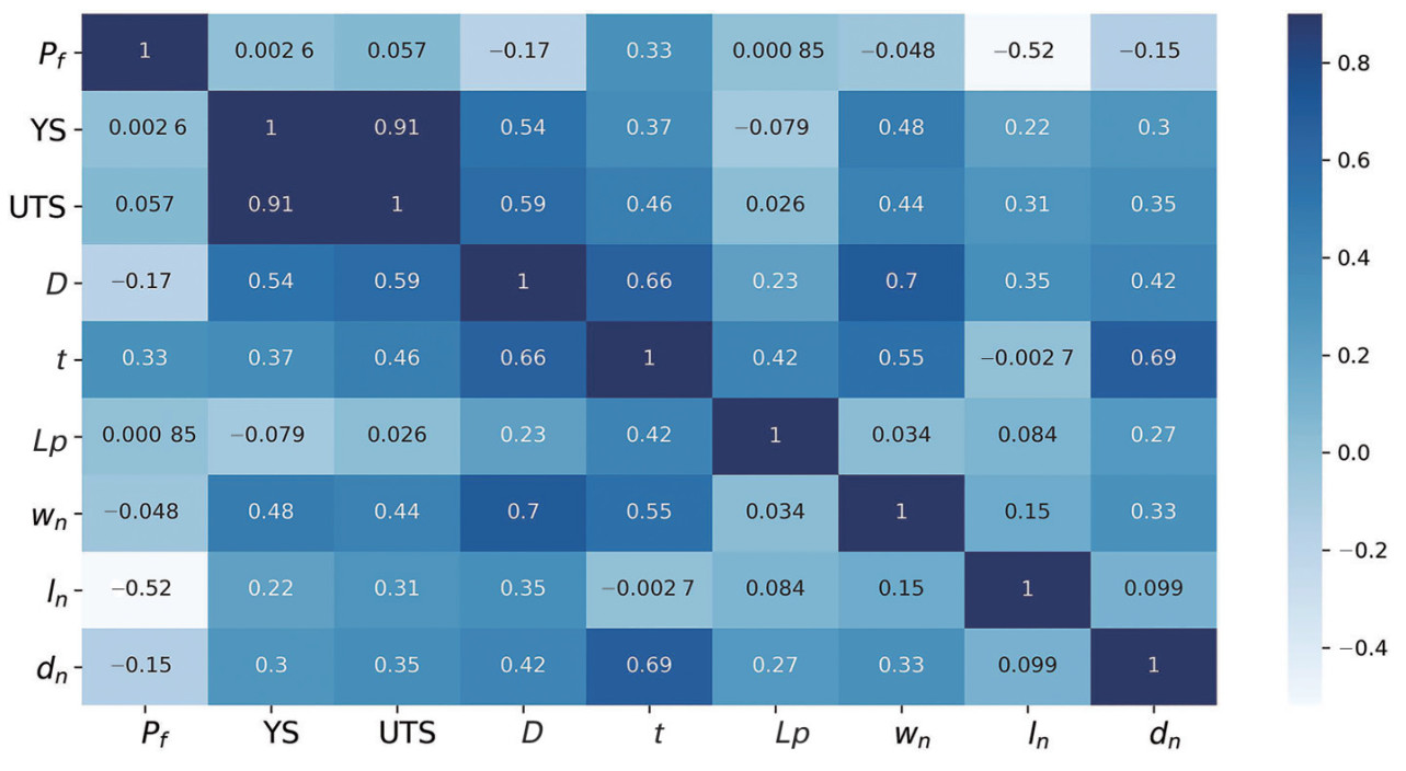Figure  7  Correlation coefficients among pipe burst pressure and pipe test features

Download: Full-Size Img

The one-hot transformation is performed to convert the categorical variables into numeric indicators. Either 1 or 0 is used to specify the presence of the variable attribute. For instance, the material type attribute of a pipe specimen with X60 material is designated as 1, whereas all the other material type attributes are assigned 0. Three categorical features, namely, corrosion defect method, material type and corrosion orientation, are selected for utilizing. Among these features, the corrosion defect method is categorized as machined corrosion, nature corrosion and intact without corrosion. The corrosion orientation is categorized as four types, including long type, hoop type, angled type and intact type. Other categorical features such as shape, notch location, pipe type are not considered due to the limitation of data size. Moreover, we noticed that there is a single sample with the material grade of A25, which has been intentionally removed. Note that the intact specimens are also added for training.

For the model training by ANN in this paper, we have obtained 21 features after a meticulous data analysis, including material yield stress YS (σ_y), material ultimate tensile stress UTS (σ_u), outer diameter (D), pipe thickness (t), corrosion length (l_n), corrosion depth (l_d), corrosion defect method (intact type, machined type, and nature type), corrosion orientation (angled type, hoop type, intact type and long type), and material categories (B, X42, X46, X52, X56, X60, X65 and X80).

5.2   Data exploration for the training by SVM and linear regression

In order to improve the accuracy of learned models by SVM and linear regression algorithms, a data transformation is conducted in this section. Figure 8 shows the density distribution of burst pressure and its KDE (kernel density estimation). In this way, we can check the skewness of data, which is a measurement of the asymmetry of the probability distribution of features/target about their mean values. A right-skewed distribution which is concentrated on the left side of the histogram is observed, as seen in Figure 8 (a). A skewness of 0.543 is computed for the pipe pressure. Hence, a logarithm transformation is performed to transform the data distribution into a normalized distribution. Note that the corresponding inverse transformation is needed for the predicted burst pressure when using the learned model.

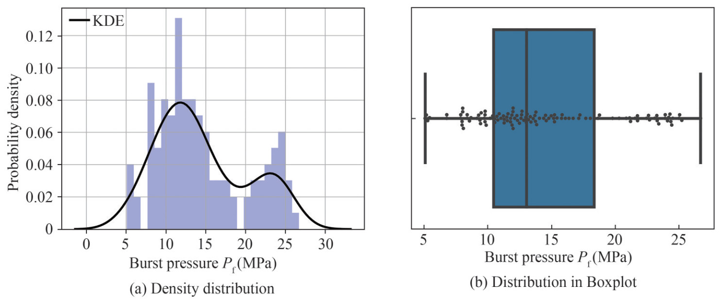Figure  8  The distribution of burst pressure

Download: Full-Size Img

With the same data analysis and visualization strategies, other features of pipe tests are explored. It is found that the features such as pipe thickness (t), outer diameter (D), corrosion depth (d_n) and corrosion length (l_n) have large skewness (larger than 1.0). Thus, the Box-Cox (Box and Cox, 1964) power transformation is applied such that the non-normalized distributed data are all transformed into a normalized-like distribution. Figure 9 shows an example of the feature distribution under the situation before and after transformation, respectively. For clarity reason, only one example of the corrosion depth is illustrated.

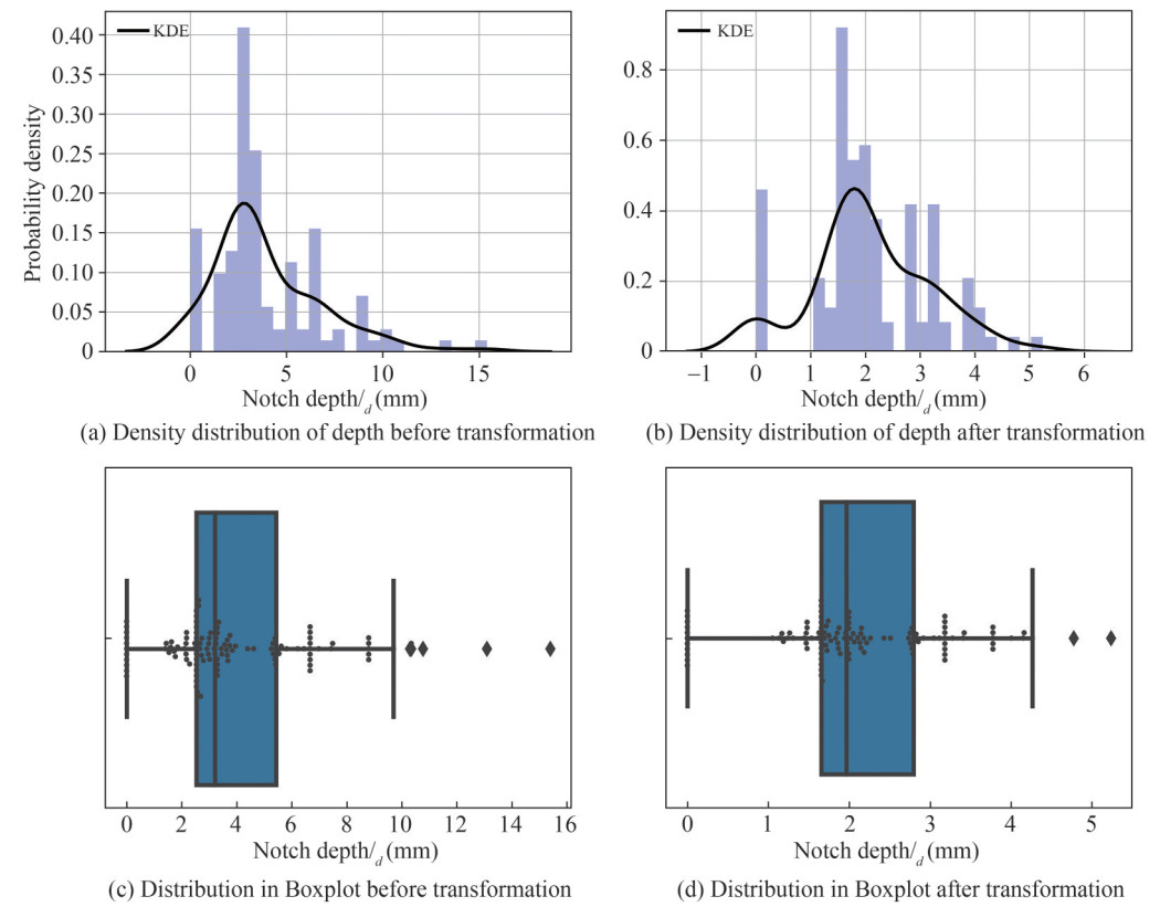Figure  9  The distribution of the corrosion depth before and after transformation, respectively

Download: Full-Size Img

6   Results and discussions

In this section, different models for the prediction of burst pressure of corroded pipelines are trained by the three algorithms, as discussed in Section 2. Hyperparameter tuning is first conducted to find the best learning parameters. Meanwhile, a parametric study is performed to study the effect of critical learning parameters on model accuracy. Prediction results of all the experimental specimens are computed and then compared through both standards and proposed numerical models. The accuracy of each learned model is discussed based on bias-variance trade-off. Note that all the numerical calculations, data analyses and model training in this paper are performed based on open-source Python libraries, including NumPy, Pandas, Matplotlib, SciPy, Scikit-learn, Keras and Tensorflow modules.

6.1   Prediction results through engineering standards

The engineering standards, as discussed in Section 4, are first adopted for the prediction of test specimens. Only the data in training and validation set are deployed. Eleven intact specimens without corrosion are removed for results comparison. Note that there is no need to differentiate the prediction results in training set and validation set since the formulas in standards are not intentionally fitted by any of these dataset.

Figure 10 (a) shows the comparison results of pipe burst pressure between predictions and experiments. It shows that there are 37 out of 90 non-conservative predictions based on DNVGL-RP-F101 (DNV, 2017). Here, the nonconservative means that the prediction values by the empirical formulas are larger than the real values from experimental tests, which may cause unsafe consequence in practice. The largest discrepancy reaches as much as 33.09% for the specimen S.N.42 (X60) in Mok et al. (1991) (among all specimens with longitudinal corrosion). The estimation of specimens with angled corrosion has a larger discrepancy, as shown from S.N.34 in Mok et al. (1991) with an error of 72.22%. For the predictions in ASME B31G (ASME B31G, 2012), only 5 out 90 specimens are non-conservative. The largest discrepancy reaches 39.1% for the specimen S.N.109 (X80) in Chauhan et al. (2009) (among all specimens with longitudinal corrosion). In the modified ASME B31G, 19 out of 90 specimens are non-conservative. The largest discrepancy reaches 30.01% for the specimen S. N. 8 (X60) in Benjamin et al. (2000) (among all specimens with longitudinal corrosion).

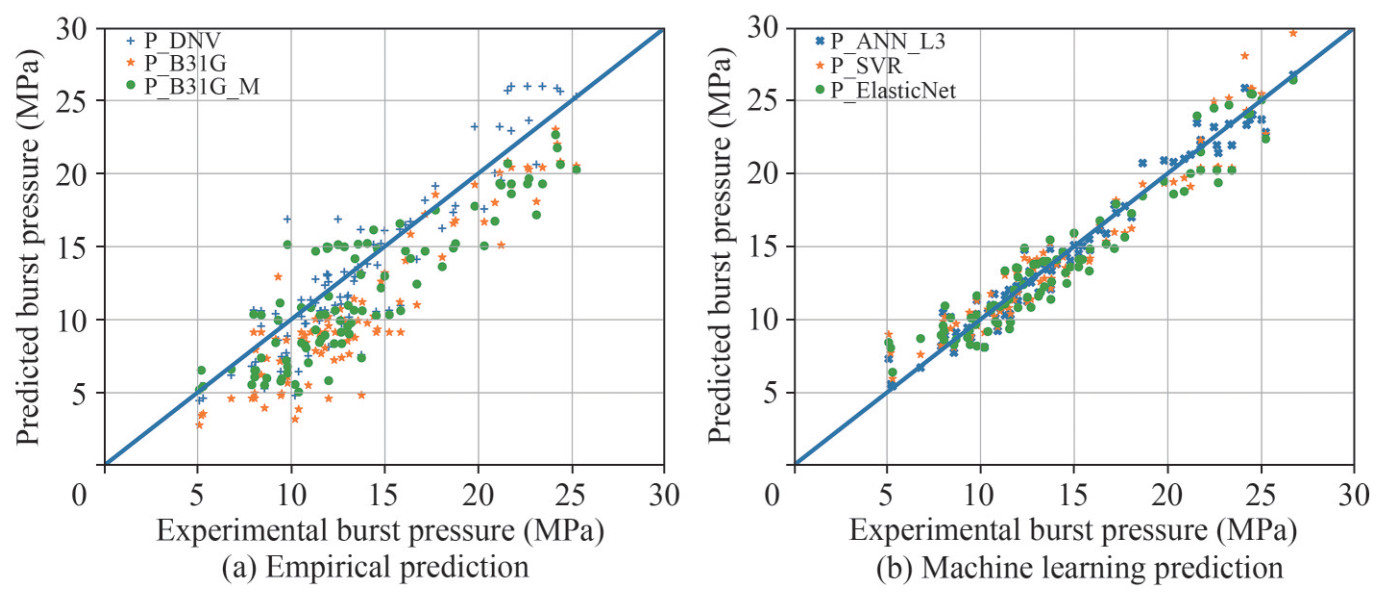Figure  10  Comparison of pipe burst pressure between predictions and experimental tests

Download: Full-Size Img

The empirical formulas also present different performance in terms of different material grades. As seen in Figure 11, it graphically compares the distributions of predicted burst pressure of pipes with different material grades using box plots. Each category of pipes is displayed in a statistical way, including the minimum, the first quartile, the median, the third quartile and the maximum. Outliers are displayed. We found that the prediction discrepancies are relative large for pipes with material grades in lower strength (e.g., B and X42) when comparing with the standards results (P_DNV, P_B31G, and P_B31G_M) and the test results (P_EXP).

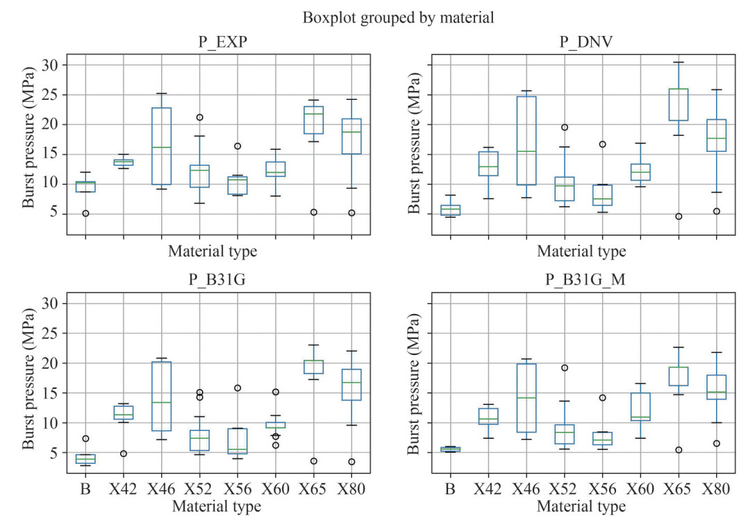Figure  11  Distribution of predicted dataset of pipe burst pressure with respect to different material type (the labels of X ticks are shared)

Download: Full-Size Img

A more refined comparison in terms of R² and MSE is conducted to quantify the estimation accuracy of empirical formulas in standards. The corresponding prediction accuracy through empirical formulas is presented in Tables 3 and 4, respectively. As we can see, the overall R² are 0.765, 0.46, and 0.612 for DNV, B31G and B31GM, respectively. The corresponding MSEs are 5.62, 12.92 and 9.28, respectively. The errors vary when it comes to individual sets with different material grades. Negative R² value occurs for the predictions of pipes with material grades of B and X42. Such poor performance implies the limited generalization ability of empirical formulas to new cases. The reason is mainly due to the small number of features when the formulas were proposed for practical use. Although conservatism rather than accuracy is more concerned in engineering practice for safety reason, these results imply that there is a space for existing engineering formulas to be improved.

6.2   Prediction results through ANN

In this section, the best prediction model is learned through an exhaustive grid search based on hyperparameter tuning. A cross-validation generator is used to randomly shuffle the pipe dataset, splitting the data into 10 independent subsets, including 9 sets for model training and 1 set for model validation. As a result, for every set of hyperparameter, it produces 10 training models with 10 different validation results. In order to improve the accuracy, the robust scaling method to normalize feature values is used before model training. Note that the test/validation dataset must use the identical scaling as the training set for predictions. A parametric study about the effect of neural layers on model accuracy is conducted for the burst pressure prediction with ANN.

The hyperparameter tuning is conducted on the model parameters in terms of optimizer types, initialization strategies for weigh matrix, the number of epochs and the number of mini-batches. An overall of 960 fitting models are simulated in order to obtain the best tuned hyperparameter. In addition, 50 models are trained based on a grid search in terms of the number of neural layers when fixing other hyperparameters. It is found that the best hyperparameters consist of three neural layers, 450 epochs (an epoch represents one iteration over the entire dataset), 2 mini-batches (the number of batches the dataset splitted), "normal" strategy for the initialization of kernel weights and "Adam" optimization algorithm. The corresponding best model for pipe burst strength prediction by ANN is trained accordingly. As shown in Table 5, the R² of three layers NN is 0.969, with the highest validation accuracy of 0.545.

For the parametric study on neural layers, five models are considered here, including a two-layer model (16, 1), a three-layer model (16, 8, 1), a four-layer model (16, 12, 8, 1), a five-layer model (16, 12, 8, 4, 1) and a six-layer model (16, 12, 8, 4, 2, 1). The numbers inside parentheses are the corresponding number of neurons in each layer. As a result, each model contains the number of model features of 369, 497, 669, 701 and 709, respectively. Figure 12¹ presents the diagram of loss values in terms of MSE with respect to the number of epochs during training, which indicates a good convergence for all the trained models by ANN. All the trained accuracy in terms of R² and MSE is listed in Table 5 for comparison. With the increase of neural layers (from L2 to L6), the accuracy in training set (R²_train) increases as expected. However, the validation accuracy first increases, and then decreases with the increase of model complexity. It implies a high variance occurs. The best learned model with three neural layers (L3) for the prediction of pipe burst pressure has the best general performance.

¹Note that the legend Val_loss_L3 denotes the loss of validation set with 3 layers, while the Loss_L2 denotes the loss of training set. Others are similar.

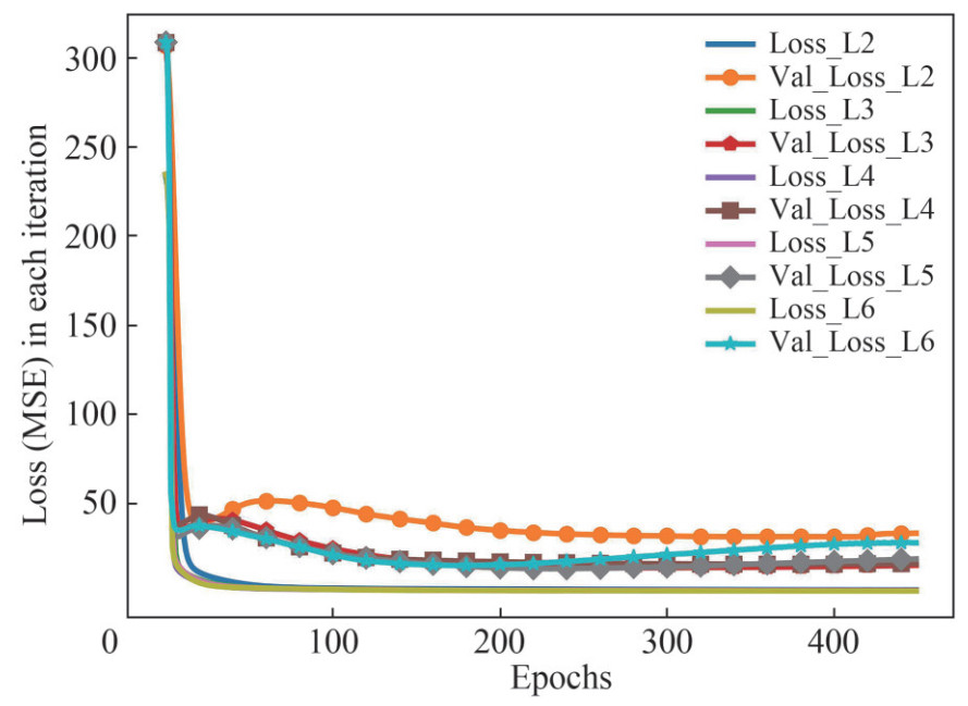Figure  12  The diagram of loss value in terms of MSE with respect to the number of epochs during ANN traning

Download: Full-Size Img

6.3   Prediction results through linear regression

In this section, three types of regression methods accounting for various regularization strategies including Ridge, Lasso and ElasticNet are utilized for the model training.

The learned linear regression model by Ridge algorithm is showed in Eq. (22), where the parameters with "Id" symbol are the categorical features after one-hot transformation (details are described in Section 5.1). When using this equation to predict a corroded pipe with X42 material type, for instance, the one-hot parameter Id_X42 will be set to 1 and all the other parameters within the material categorical feature (e.g., Id_X46) are set to 0. Other categorical features are similar. The best hyperparameter λ for L² regularization in the training model is 1.0. For the Lasso algorithm, the corresponding learned weights are −0.050, 0.324, −0.459, 0.469, −0.136, −0.339, −0.349, 0, 0, 0.308, −0.032, −0.061, 0.001, 0, 0.012, −0.066, 0, −0.043, −0.212, 0.009 and 0.002 with the bias of 2.745. The parameter sequence is the same as Eq. (22). The best hyperparameter λ for L¹ regularization is 0.001 6. Likewise, for the ElasticNet algorithm, the corresponding learned weights are −0.069, 0.341, −0.462, 0.480, −0.149, −0.357, −0.403, 0, 0, 0.332, −0.077, −0.056, 0.001 4, 0, 0.006, −0.086, 0, −0.050, −0.206, 0.016 and 0.021 with the bias of 2.747. The best hyperparameters of regularization are 1.0 and 0.000 9. As we have noticed, some features are automatically set to zero when adopting the L¹ regularization strategy in both Lasso and ElasticNet. Table 6 lists the different accuracy of learned models by applying different regularization penalty. The learned model by ElasticNet algorithm has the highest training accuracy with a high validation accuracy as well. The comparison results indicate a good performance of the pipe burst prediction models by just using a linear regression.

6.4   Prediction results through SVR

Three tuning hyperparameters in SVR, including regularization coefficient (C), kernel width coefficient (γ) and the types of kernels, are used for grid search. Similar with the way in Section 6.2, a cross-validation generator is used to randomly shuffle and split data. As a result, an overall of 1 470 training models are trained in order to learn the best hyperparameters. The simulation results show that the best combined hyperparameters consist of C=50, γ =0.01 and the RBF kernel (Gaussian transformation). The estimation accuracy of models with different kernels is listed in Table 7. It is observed that the best model with RBF kernel has a good general performance accounting for both the validation and test performance.

6.5   Model comparisons and discussions

In this section, a comprehensive comparison of each learned model for the pipe burst strength prediction is performed. The possible intelligent application of the improved models is explained. Discussions are presented in terms of model limitations.

Figure 10 (b) shows the comparison results of pipe burst pressure between the predictions and the experiments. The corresponding predicted strength is listed in Table 8. Only nine specimens are presented for clarity reason. It is obvious that the prediction scatter has been largely improved compared with the results from empirical formulas. For instance, B31GM provides a prediction with −68.67% discrepancy for sample S.N.9, whereas the SVR method gives a more accurate prediction with discrepancy of −10.54%. Figure 13 explicitly illustrates the comparison results between predicted values through all the best learned models and the true values of experimental test. All the test specimens are sorted with respect to their series numbers (S.N.). The experimental values of all specimens are connected by a black line so as to have a clear visualization. Prediction results match very well with the experimental tests in general. As observed, there are outliers on specimen S.N. 61 with material grade X65, with the relative prediction errors (|Predicted value-True value|/True value) of 26.1%, 16.35% and 7.22% for the trained models by ElasticNet, SVR and ANN, respectively. The largest relative error occurs on the specimen of S.N. 11 with material grade B for all the learned models. The errors are 65.7% for the learned model by ElasticNet, 76.2% by SVR and 43.4% by ANN, respectively. The reason is due to the limited number of training pipes with grade B, which will be improved in further research by transfer learning.

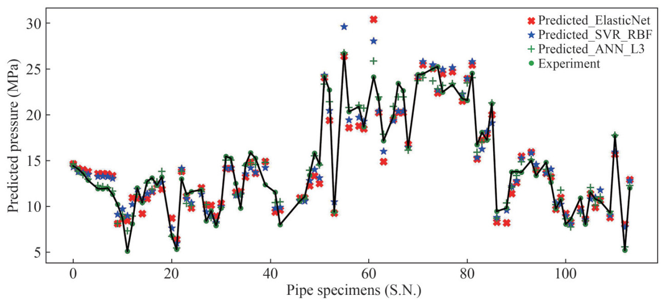Figure  13  The comparison diagram between predicted values through learned models by supervised machine learning (three-layer ANN, SVR with RBF kernel and ElasticNet) and the experimental results

Download: Full-Size Img

Figure 14² shows the comparison diagram of learning accuracy in terms of R² and MSE for both the learned models and the empirical formulas in standards. It is found that the learned models by the ANN algorithm have the highest training accuracy, but with a relative low validation accuracy. This phenomenon indicates that overfitting appears. Compared with the ANN models, the training accuracy of models by SVR and LR slightly decreases but with a relative high validation accuracy. As a result, the generalization of these training models has been improved. In addition, accounting for the accuracy results from test set, as seen in Tables 5, 6 and 7, the trained models by linear regression provide the best prediction performance among all the proposed models. Note that, due to limited data size, the test set has not been used in this work for model performance evaluation. The generalization ability of models should be further improved.

²Note that L6 denotes the ANN model with six neural layers, while It should be Li_R represents the Ridge model. Besides, it should be SVR_P denotes the SVR model using a polynomial kernel. Other signs are similar.

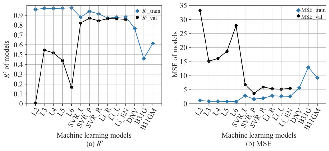Figure  14  The diagram of learning accuracy for learned models with different machine learning algorithms

Download: Full-Size Img

Compared with the improved models by machine learning algorithms, it cannot be denied that these empirical formulas from standards are easier to apply by hand due to less features and simpler formulas structures. However, these empirical models present a relative low performance in terms of accuracy and generalization. The DNV standard for corroded pipelines has a better performance than the ASME B31G. Meanwhile, the Modified B31G formulas have further improved the prediction ability of burst strength of corroded pipelines compared with the formulas in B31G. The developed models by machine learning algorithms imply a promising utilization of intelligent prediction in future, which provides a solid foundation for our further work.

The improved prediction models by data-driven method in this paper can facilitate an intelligent decision-making of corroded pipelines accounting for all the measured data. In the foreseeable future of digital operation in pipeline domain, these models can be easily integrated into software for the burst strength prediction and real-time monitoring. A brief procedure of such potential applications is listed as follows.

• Integrate the prediction models into pipe monitoring software (ensemble strategy is used when necessary);

• Collect all the static pipeline features such as pipe diameter, thickness and material level;

• Collect all the real-time corrosion features (angle and length, etc.) on pipelines by sensors or cameras;

• Automatically calculate the burst pressure and set an alarm when violating the prescribed safety factors.

The models in this paper have been initially demonstrated to be effective with good generalization ability. However, it should be noted that model limitations still exist due to the limited number of training data. More cases are needed to further validate the accuracy of these models. In the future research, the transfer learning should be applied to improve current models when more data are found. Note that the yield stress and UTS of pipes in reality are not easy to obtain rapidly. Thus, these features could be replaced by parameters such as the SMYS (Specified Minimum Yield Strength) from pipe material standards instead. Further research is needed to be done in order to introduce proper correction coefficients for such replacement.

7   Conclusions and future work

In this paper, a novel research on the burst strength prediction of corroded pipelines has been conducted based on data-driven methodologies including three typical machine learning algorithms. Compared with the conventional methods, the work has provided an alternative research fashion on pipeline strength investigation. A single rectangular corrosion defect located on the specimen center was considered. Pipe data were obtained from existing experimental test of corroded pipe specimens and were explored carefully based on various data analysis techniques. Improved prediction data-driven models with high performance were proposed. Parametric studies on ML training parameters were performed. The prediction results from existing engineering standards were compared to the proposed models. The conclusions of this paper are drawn as follows:

1) The ANN with three neural layers has the highest training accuracy for pipe burst strength based on limited dataset, but also with the highest variance.

2) The SVR provides a slightly lower training accuracy than the ANN with limited dataset. However, the high variance is largely improved.

3) The proposed pipe models based on limited dataset by LR present the best performance in terms of generalization ability among the three algorithms.

4) Compared to the trained models by machine learning algorithms, empirical models from engineering standards show a relative low performance. Despite the fact that the empirical formulas are simple and easy to use by hands, there is still some space to be improved with respect to accuracy and generalization ability.

Due to the limited number of data in engineering practice, the performance of trained models by data-driven methods will be inevitably affected. One way is to further collect effective data either from literature or conducting more pipe tests. Then, a re-training process is needed but is cumbersome and impractical. The other option is, instead of doing model re-training, to apply transfer learning for the improvement of the model performance. The improved models in this research can be therefore used as the surrogate models for transfer learning. Further research in this aspect is needed to be done.

Data availability statement

The original training data of corroded pipe experimental test and all the trained models are available from https://github.com/jiejie168/pipeBurstPressure_prediction_dataDriven