1   Introduction

Propeller design in ship propulsion systems is usually confined to the analysis of steady-state conditions, deeply submerged propellers, or open water tests. However, when precious estimations (e.g., special maneuverability) are required, a sophisticated consideration should be applied to adequately determine propeller performance. In numerical studies, such a complex consideration can be addressed by Reynoldsaveraged Navier-Stokes (RANS) solvers, such as the finite volume method (FVM) or finite element method. In these methods, the propeller behind the ship can be simulated with many details, such as the influence of the velocity wake filed of a ship (and its appendages) on the propeller. Nonetheless, RANS solvers are time-consuming methods, especially in simulating (two or more) moving objects that should be coupled with a moving-grid technique, e.g., overset method (Benek et al. 1983; Meakin and Suhs 1989; Henshaw and Schwendeman 2006).

Furthermore, inviscid approaches, such as the boundary element method (BEM)(Hess and Smith 1962, Hess 1972, Hess and Valarezo 1985), are efficient techniques for predicting the pressure force of lifting bodies. In recent decades, many scientists have studied and developed boundary element formulations to improve their accuracy. Politis (2004) used a three-dimensional (3D) unsteady BEM to solve flows around a marine propeller. He used the time-stepping method (TSM) to model the vortex sheet emanating from each blade trailing edge and showed that this approach could produce a very stable rollup wake pattern related to the prescribed wake shape (PWS) and wake relaxation method (WRM). Politis (2011) applied his solver to a wide range of working conditions of a propeller, such as a propeller in a straight/circular course, an azimuth propeller, and a ducted propeller in a circular course. He also showed that the burst starting of a propeller may be modeled with a good agreement through his method compared with experimental data. Subsequently, Politis (2016) introduced an artificial viscosity filtering technique to a domain that suppresses small-scale instabilities and leaves large-scale vortices. These vortices were used to determine the rollup pattern of free wake vorticity. He applied his model to a number of flows around lift-producing configurations, such as a burst starting propeller. Finally, he concluded that this model could be used as an attractive alternative in the case of preliminary force predictions. Durante et al. (2013) compared different hydrodynamic models to analyze the load delivered by the marine propeller PROP 3714 in an axial non-uniform wake flow to find a reliable and fast model to balance the accuracy and computational time. They used the BEM model as a reference point for their calculations. Wang et al.(2016) described four different numerical methods to implement wake alignment algorithms for a marine propeller in steady-state flows. They applied all four methods to calculate the performance of a KP505 propeller. To show the wake geometry, a rectangular foil was simulated, and the wake shape was compared. In a similar effort to determine an efficient method to solve off-design aspects related to ships and their propulsion system in the earlier design stages, Gaggero et al. (2019) investigated the capability of the BEM and blade element momentum theory (BEMT) propeller solver to predict propeller performance in a maneuvering condition. The comparison between the BEM and BEMT was performed behind the hull condition of a twinscrew ship. The results show that although the BEM is at least one order slower than the BEMT, it is more accurate and could predict propeller performance behind ships with acceptable accuracy.

Meanwhile, BEMs have been extensively improved, but designers still need the RANS solver. This fact motivated scientists to combine the efficiency of the BEM with the accuracy of the RANS solver to reduce the numerical effort without compromising the predictive accuracy. Greve, Wöckner-Kluwe et al. (2012) analyzed the dynamics of a single-screw propeller ship in seaways by combining the BEM and RANS solvers. In their algorithm, the propeller force was computed in the BEM solver, while the inflow condition for the propeller was provided by the RANS method. Although the WRM was used to simulate propeller vortex sheets, the propeller thrust and ship resistance were the main investigated parameters in their work (no wake shape was shown). Rijpkema et al. (2013) numerically investigated the propeller–hull interaction of the wellknown single-screw Kriso Container Ship (KCS) using a combination of the steady-state RANS solver for the ship hull flow and the unsteady potential method for propeller loading. Compared with experimental data, this approach predicted the propeller thrust forces to be within 2% to 3%, with a significant reduction in the computation time. Conversely, Queutey et al. (2013) tried to find an efficient way to simulate marine propellers behind a ship. They compared a full RANS solver with a steady coupled RANS-BEM to predict the propulsion performance of a propelled ship. Code PRO-INS, which was developed by CNR-INSEAN, was applied as the BEM computational model, while the unstructured finite volume solver ISIS-CFD was applied as the RANS approach. The STREAMLINE tanker and propeller were considered in the validation test case. Because of the massive computation time, the RANS simulation was performed only for the design speed, while the steady hybrid RANS-BEM computations were performed for the speed range. They show that the CPU time for the steady RANS-BEM coupling is divided by a factor of 50 as compared to the full RANS (with reasonable accuracy). Hence, it can be used for preliminary design purposes. Gaggero et al. (2014) analyzed the reliability of different numerical approaches (BEM and RANS solver) to predict the performance of the well-known highly skewed marine propeller Seiun-Maru, which operates in different wakes. In their BEM model, a frozen wake geometry was adopted as the result of the steady alignment with the propeller in a uniform inflow. They used StarCCM+ commercial software as a RANS solver. The results showed that the numerical code presents a good capability in predicting propeller characteristics and pressure distribution when the thrust identity approach is adopted. Rao and Yang (2017) presented a hybrid approach (panel method and RANS) to predict the self-propulsion performance and effective wake field of an underwater vehicle. Numerical simulations were performed for the full appendage SUBOFF submarine. They used two different ways to evaluate the wake field and showed that the effective wake fractions are approximately 4% larger than the nominal. Conversely, Gaggero et al. (2017) presented a coupled BEM/RANS approach to simulate the self-propulsion prediction of a KCS hull. The total hull resistance was computed by the RANS solver without a propeller, but they used the BEM method for propeller simulations, which was much faster than the finite volume moving mesh technique (e.g., overlap grids). Gaggero et al. (2019) presented a propeller solver based on the BEM to analyze the propeller performance in different flow conditions. The nominal wake of a twin-screw ship was first evaluated using the unsteady commercial RANS (Star-CCM+) solver, and then it was used as an offline input to the propeller solver. The wake shape of the propeller was modeled by the PWS method. They also compared the results to a steady-blade element approach to determine a fast and less time-consuming method to simulate propellers.

In the current study, a numerical solver was developed based on the coupled BEM/RANS approach to solve flows around twin-screw marines, considering the influence of the ship wake field. The main motivation of this study is to combine the advantages of both methods to reduce the computational time without compromising the predictive accuracy.

In the BEM solver, each propeller is supposed to consist of lifting bodies (blades). The TSM was used to simulate the freely moving unsteady trailing vortex sheet, which emanates from the trailing edge of each blade. This is the main novelty in combining the BEM and RANS solvers. This approach correctly simulates and visualizes the vortex blade-wake interaction at each time step. The BEM solver was applied to a highly skewed controllable pitch marine propeller, and the results were compared with experimental data.

Meanwhile, in the RANS solver, two main equations must be simultaneously solved. The FVM was used to discretize the unsteady Navier–Stokes (NS) equation in arbitrary unstructured grids. The second equation is the scalar transport equation, which is solved to calculate the volume of the fraction. The high-resolution compressive interface capturing scheme for arbitrary meshes (CICSAM) approach was applied to capture the fluid interface on the meshes with an arbitrary topology. Combining the two equations with rigid body motions makes it possible to simulate ships in calm water. The RANS solver was also validated by calculating the resistance on a high-speed catamaran and fully appended 50m oceanography research vessel (RV50) in calm water. The results were compared with a towing tank test and similar work. Finally, the coupled approach was applied to estimate the twin propeller performance behind the ship. The wake sheet pattern was also shown to be influenced by the ship wake field, which was consequently affected by ship appendages.

2   Governing equation

2.1   BEM method (inviscid solver)

As pointed out earlier, the propeller forces were calculated using the BEM. Considering incompressible, irrotational, and non-viscous flows, the BEM is based on the solution of a Laplacian equation:

where ϕ(x, t) is the velocity potential in the discretized domain. ϕ(x, t) can be written as a linear combination of fundamental potential functions, such as sink/source, dipole, and vortex, which could be computed on each cell center. Based on Green's second identity, the 3D problem of Eq. (1) can be solved as a simple integral problem on the boundary surface of the computational domain:

where $\lambda=\frac{1}{r}$ is defined as the fundamental solution for the 3D potential flow. n and r are the unit normal vectors of the panel (pointing outward of the body) and the distance between the source point and field point, respectively. As a result, Eq. (2) can be written in the form of

The surface cells in the discretized domain are divided into three main zones. Depending on the related zone, each cell is treated differently. We consider a three-blade propeller, which operates on an unbounded flow, as shown in Figure 1. Surface cells are divided into the following three main zones:

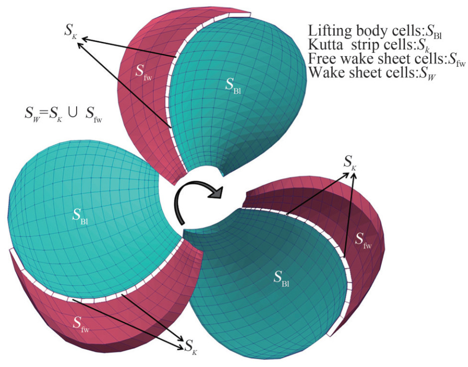Figure  1  Cell types in the propeller

Download: Full-Size Img

Zone 1 (blade/lifting cells (S_Bl)): These cells are contributed to generating the lifting force. The wake sheet is generated from the leading edge of lifting cells.

Zone 2 (Kutta-strip cells (S_k)): These cells are located in the first row and are adjacent to the trailing edges of the blade body.

Zone 3 (free wake sheet cells (S_fw)): These cells include all cells on the wake sheet except Kutta-strip cells.

The wake sheet cells are all cells in the second and third zones (S_W = S_k ∪ S_fw).

The discretization of Eq. (3) is shown in Eq. (4) (Politis 2011):

The first and second terms on the right-hand side are obtained from the previous time step; hence, they can be explicitly calculated (Najafi and Abbaspour 2017). The dipole intensity over body cells (ϕ) and Kutta-strip cells (μ) should be calculated by forming a system of linear equations. The pressure-type Kutta condition states that pressure should be continuous when the flow approaches the trailing edge from either the suction or pressure sides. In this study, the linear Morino-type Kutta condition was used at each time step:

Calculating Eq. (4) for all body and Kutta cells leads to a linear system of equations in the form of (AX = B), which could be solved by common iterative methods. This equation also gives the dipole intensity over the body and Kutta cells.

As mentioned before, the TSM was used to investigate the wake sheet pattern in all simulations. In the TSM scheme, the wake sheet is developed through time, which implies that at each time step, a new row of nodes is added while the position of previous nodes is updated. It is thus necessary to calculate the velocity of wake sheet nodes at each time step. The velocity of wake sheet nodes is referred to as the perturbation velocity, which could be calculated by taking the gradient of Eq. (4) as follows (Zhu et al. 2002):

The integral zones for the first three terms are shown in Figure 2. The fourth term is calculated over the lines bounding the free wake sheet. Moreover, it is a line integral over the bounding of the wake surface and is depicted in Figure 2 for a single blade (Katz and Plotkin 2001). If the last term is ignored, the starting vortex and wake rollup pattern will not be correctly formed.

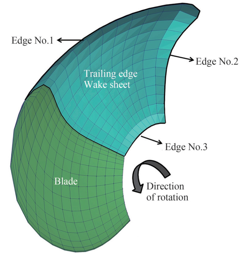Figure  2  Boundary lines of the free wake sheet

Download: Full-Size Img

After calculating the perturbation velocity for all wake sheet nodes, the new position of the wake sheet can be calculated by a simple linear formula as follows (Zhu et al. 2002):

where V_rel is the relative velocity of each cell:

When the potential velocity distribution is calculated over each body cell using the unsteady Bernoulli equation, the pressure can be computed by Najafi and Abbaspoor (2019).

The hydrodynamic force and moment over each blade are calculated by integrating the pressure (normal stress) and virtual friction (shear stress) forces over the body. More details can be found in Politis (2005).

2.2   RANS solver (viscous method)

The two-phase-flow 3D NS equation was used as the governing equation for the viscous solver to simulate flows around the ship hull. In almost all marine problems, the Mach number is less than 0.3, so the NS equations are used in their incompressible form. Accordingly, the momentum and continuity equations can be simplified as follows:

In cases where there are two-phase fluid simulations, one should solve the volume fraction transport equations:

In this equation, α is the fractional value demonstrating the amount of water in the cell:

Generally, Eqs. (10) and (11) should be solved simultaneously. For this purpose, the fluid density and viscosity of each cell in the computational domain can be expressed as a function of the volume fraction α as follows:

where subscripts 1 and 2 denote water and air, respectively.

2.2.1   Discretization of NS equations

In the present study, the FVM was applied to discretize the NS equations. Integrating these equations over each control volume can result in the following equation:

For the fluid velocity u_i, the diffusion term (the first term on the right-hand side of (14)) was discretized using overrelaxed interpolation (Jasak 1996):

To discretize the convection term (the second term on the left-hand side of (14)), the fluid velocity at the control volume faces needed to compute fluxes. This condition can be evaluated as follows:

To calculate u_f, the Gamma interpolation scheme was used, which was introduced by (Jasak 1996).

The Crank–Nicholson scheme was also used for the time discretization of diffusion and convection terms in Eq. (14).This scheme has second-order accuracy and increases stability.

The pressure term (second term on the right-hand side of (14)) is discretized as

where A_f is the direction component of the face area vector.

Using the common linear interpolation between two neighboring control volume centers results in severe oscillations in the velocity field. This is of great importance, especially when there are two fluids with high-density ratios, e. g., water and air. Here a piecewise linear interpolation was used, which was developed by Panahi et al. (2009).

2.2.2   Discretization of the volume of fluid equation

The finite volume discretization of the volume fraction transport Equation (11) is based on the integration over the control volumes and time step:

The first term is a simple integral form. By applying the Gauss theorem on the second term and assuming a small variation of F_f, we can derive

where α_f must be approximated on the face of each control volume. A simple interpolation results in non-physical values, leading to the use of a high-order composite interpolation. In this study, the compressive interface capturing scheme for arbitrary meshes (CICSAM) was applied (Ubbink and Issa 1999). CICSAM uses convection boundedness criteria (CBC) and ultimate quickest (UQ) interpolations by introducing a weighting factor γ_f (Gaskell and Lau 1988; Leonard 1991). This factor was evaluated according to the slope of the free surface and the direction of fluid motion (Ubbink and Issa 1999). Based on the normalized variable diagram (NVD), a normal face value was obtained (Leonard 1991):

NVD definitions are shown in Figure 3, where donor, acceptor, and upwind cells are defined according to the flow direction for each control volume face:

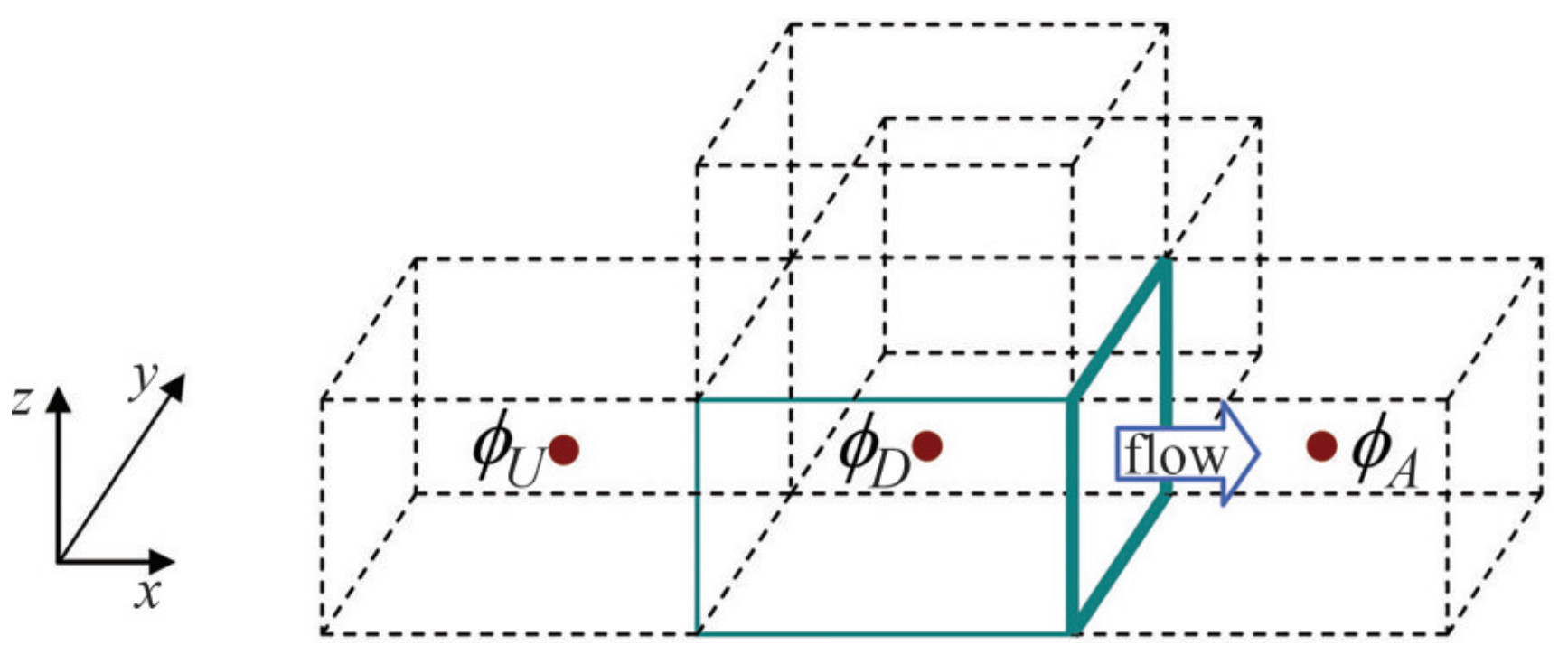Figure  3  Flow direction determines donor, acceptor, and upwind cells (Panahi et al. 2006)

Download: Full-Size Img

Substituting Eq. (20) into (21) results in the estimation of α_f

In the volume of fluid (VOF) approach, the Courant – Friedrichs–Lewy (CFL) number plays an important role in the stability of a solution. Here, the Courant number was calculated according to Eq. (22) for each cell and was set to be less than 0.2 for all two-phase flow test cases Panahi et al. (2009).

As mentioned before, a body attached mesh was used to simulate body motions. In this way, the relative velocity should be applied in all equations:

where u_fluid is the fluid velocity vector and u_body is the velocity of a moving body (which is equal to the mesh velocity).

2.2.3   Coupling of the pressure and velocity

The method used to couple the pressure and velocity fields is the modified fractional steps, which were first proposed by Kim and Choi (2000). We considered the NS equations for the velocity component u_i in its discretized form on a given control volume. The first step was to solve the first intermediate velocity (û_i) with the pressure gradient in the previous time step G_i(Pⁿ):

where

Then, the second intermediate velocity is calculated as

Using Eq. (26) results in the pressure Poisson equation, which gives a new pressure field Pⁿ⁺¹:

By writing Eq. (27) for all cells in the computational domain, a system of equations in the form of (AX = B) was obtained. Solving the system of equations, the velocity at a new time step was computed as follows:

Because this new pressure was used to calculate "modified" velocities, global mass conservation was automatically satisfied. After the calculation of all velocity components in an outer iteration, the control volume face velocity vector was calculated for the next time step from Eq. (29). It includes the effect of the pressure gradient on the calculation of the face velocity vector to overcome the checkerboard pressure in the non-staggered (collocated) arrangement:

A comprehensive in-house computational program was developed based on the mentioned approaches. More details about the implemented algorithms and their validation can be found in Pourmostafa and Ghadimi (2020b).

3   Validation of solvers

Before coupling the inviscid/viscous solvers, they should be validated separately for related test cases. Although each solver was separately validated in the different studies of (Pourmostafa and Ghadimi 2020a; 2020b), here, according to the final test case (research vessel and its highly skewed propeller), two validations of the solvers are presented. A viscous solver was used to simulate the motion of a highspeed catamaran and a 50 m research vessel (RV50) and calculate their resistance forces. The calculated resistance forces were compared with experimental towing tank data and similar works. Meanwhile, an inviscid solver was applied to predict the performance of a highly skewed marine propeller, which was designed for the same research vessel. The BEM results were compared to open water test results. In particular, in all cases, a mesh independent analysis was performed, and the best mesh size was properly selected.

3.1   Resistance and motion of a high-speed catamaran (validation of the viscous solver)

To validate the viscous solver, the motion of a high-speed catamaran was investigated at three velocities (Vel=5, 16.5, 24 kn). The main dimensions of the high-speed catamaran are shown in Table 1. Due to hydrodynamic forces, the catamaran tended to exhibit heave motions and pitching angles, which can be modeled by the developed solver with two degrees of freedom.

The computational domain was discretized by 180992 hexahedron structural grids as shown in Figure 4.

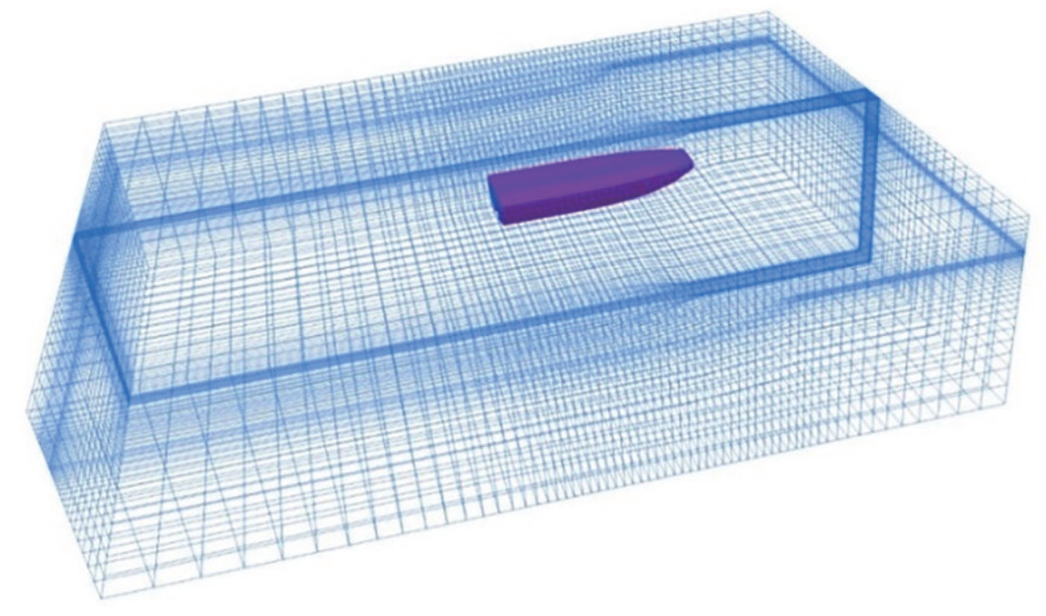Figure  4  Computational domain of the high-speed catamaran

Download: Full-Size Img

When the main hydrodynamic parameters of the catamaran become steady, the heave, trim, and resistance forces were compared with those in the similar work of Panahi et al. (2009), as shown in Figure 5.

Figure  5  Heave motion, trim angle, and resistance force of the catamaran

Download: Full-Size Img

The viscous solver could predict the hydrodynamic force and motions of the high-speed catamaran with good accuracy. The catamaran at Vel = 24 kn is illustrated in Figure 6.

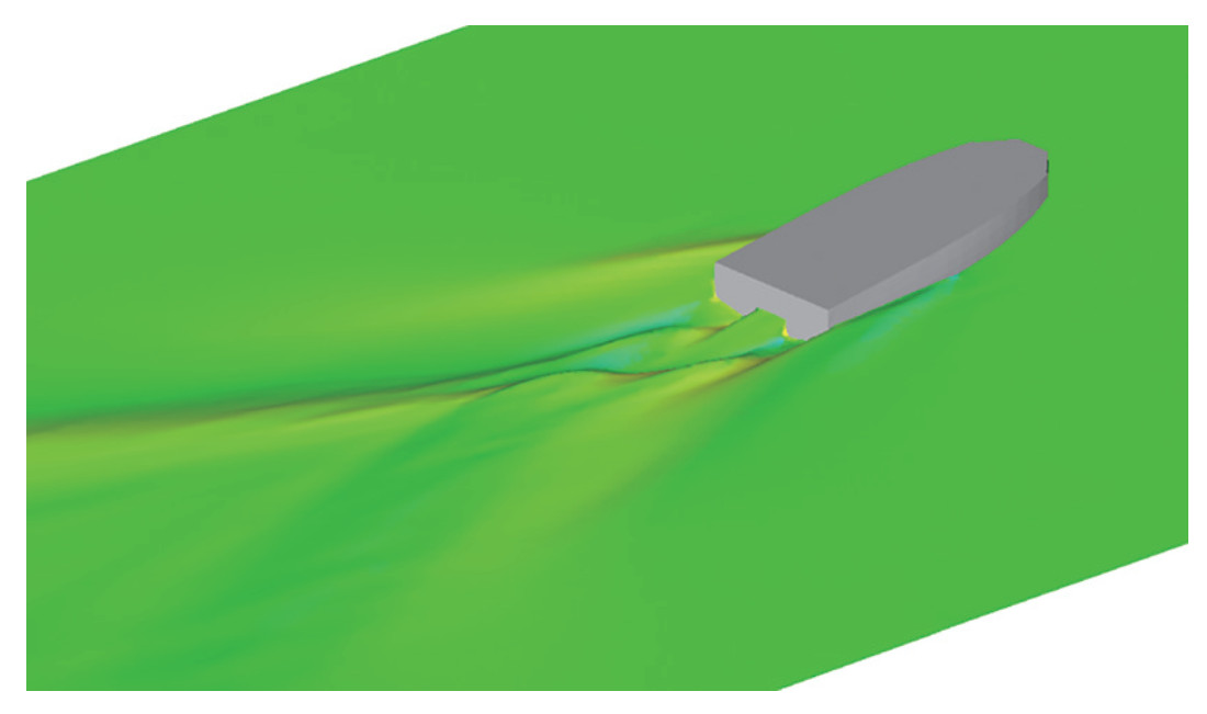Figure  6  Catamaran in a steady condition at V = 24 kn

Download: Full-Size Img

3.2   motion of RV50 in calm water (validation of the viscous solver)

RV50 is a 50 m twin propeller research vessel, which was designed for a cruise velocity of 12.3 kn. In this study, the viscous solver was used to calculate the vessel resistance in still water. Table 2 shows the main characteristic of this ship.

The computational domain is displayed in Figure 7. A total of 306222 unstructured grids were used to discretize the RV50 with full appendages, as shown in Figure 8.

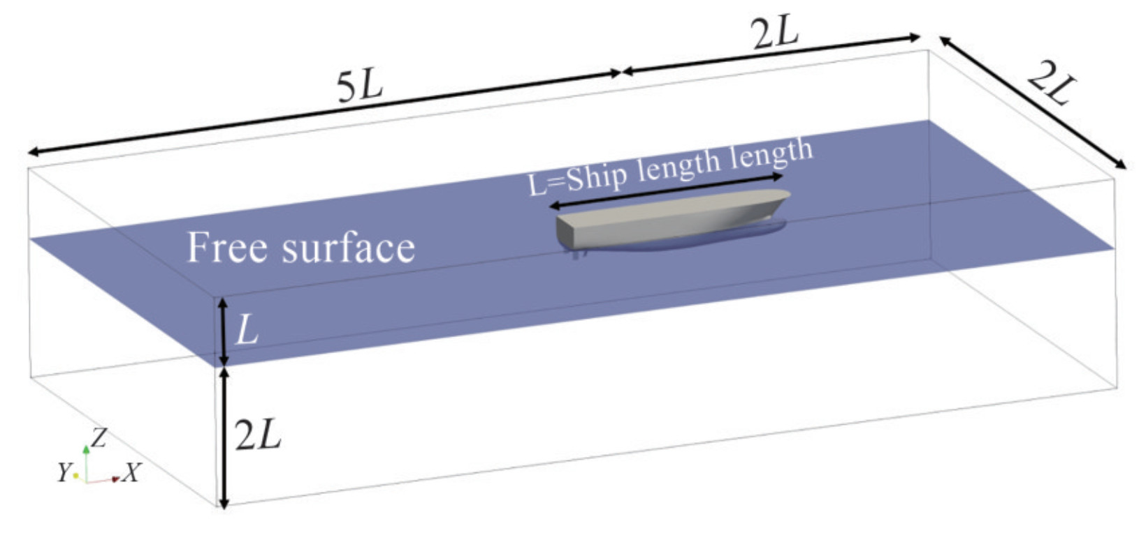Figure  7  Computational domain of the RV50

Download: Full-Size Img

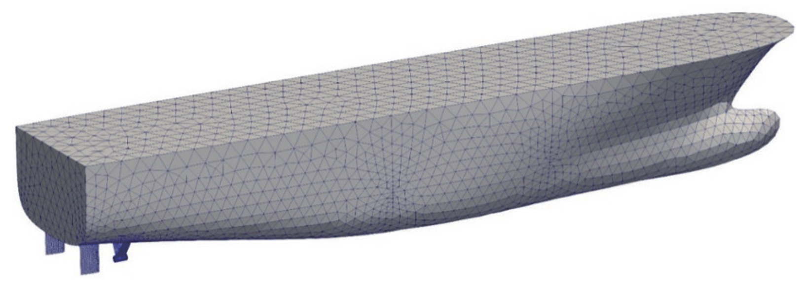Figure  8  Fully unstructured mesh used to discretize the RV50

Download: Full-Size Img

The simulations were performed at seven different velocities, and the results are compared with experimental data of (RV50 Test Report 2011) in Figure 10. The model resistance of the research vessel was measured at the towing tank of Vienna Model Basin with a wooden model on a 1: 12 scale (Figure 9), and the total resistance for the full scale was calculated using International Towing Tank Conference (ITTC) relations. In particular, minor resistance components, such as air resistance and hull roughness effects, were also added to the numerical model based on the experimental relations advised by the technical committee of the (ITTC-Recommended Procedures and Guidelines 2011). Figure 11 displays the free surface elevation near the vessel at V = 14.5 kn.

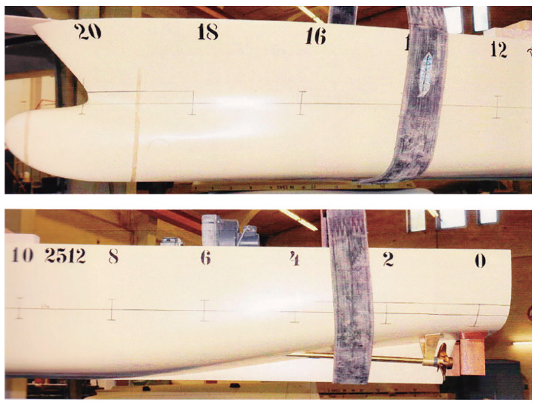Figure  9  Pictures taken from Vienna Model Basin (RV50 Test Report 2011)

Download: Full-Size Img

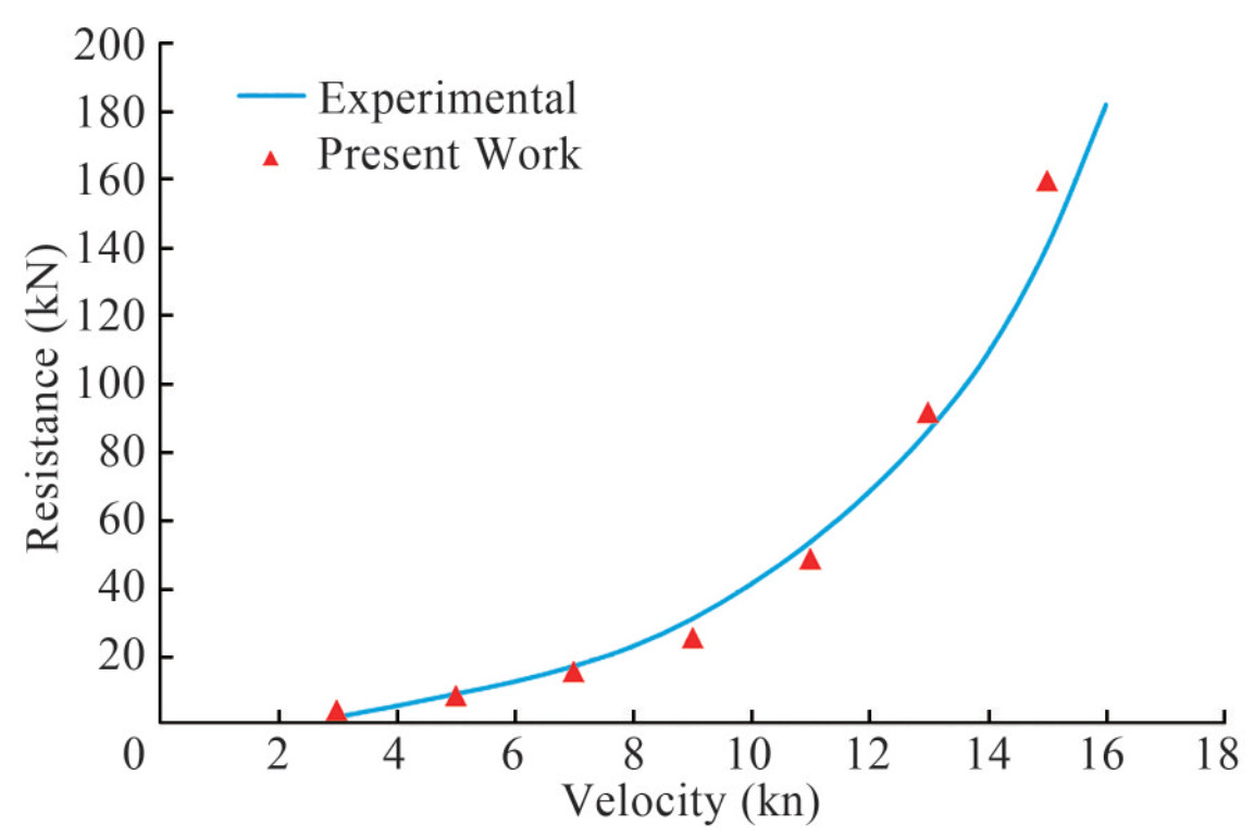Figure  10  RV50 resistance at different velocities

Download: Full-Size Img

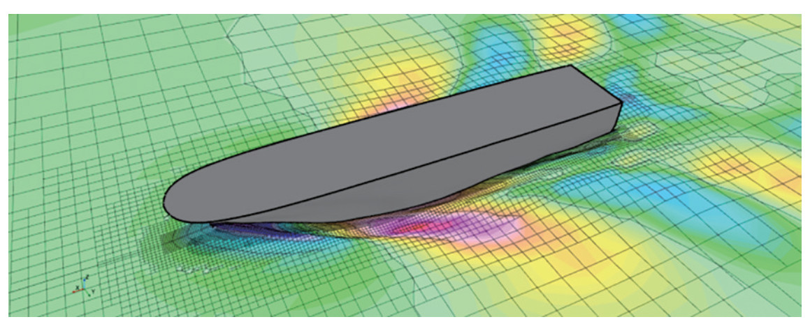Figure  11  Free surface elevation of vessel at V = 14.5 kn

Download: Full-Size Img

The wake field velocity in the propeller plane (in the absence of a propeller) is usually referred to as a nominal wake. The nominal wake of he vessel at its top speed is shown in Figure 12, which was calculated based on (Rao and Yang 2017) as follows:

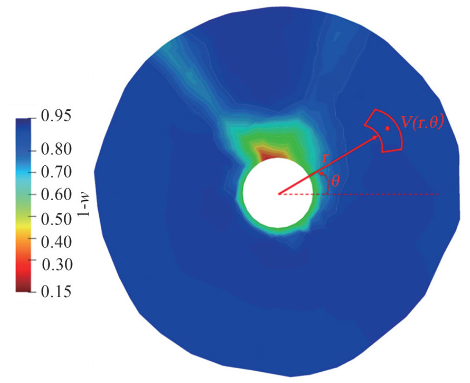Figure  12  Nominal wake of the RV50 at its top speed (V = 14.5 kn)

Download: Full-Size Img

To calculate the disk average wake fraction, one should integrate velocity in this field. In this way, infinitesimal radial elements shown in Figure 12 are defined on the propeller plane.

Having velocities on these points, the average velocity could be calculated using Eq. (30). In the present research, the computational wake was compared with an experimental value measured in the towing test using 5-hole pitot tube probes equal to w = 0.088. Table 3 shows the comparison between the results.

3.3   Performance of the RV50 marine propeller (validation of the inviscid solver)

The inviscid solver was validated through different test cases, such as the DTMB4119 and KP505 marine propellers used in Pourmostafa and Ghadimi (2020a). In this section, the validation of the RV50 propeller is presented because this propeller was used for the simulation in the coupling section. It is a controllable pitch propeller designed for the research vessel. The main particulars of this propeller are shown in Table 4.

The BEM inviscid solver was used to calculate the hydrodynamic parameters of RV50 propeller. Figure 13 shows the comparison between the computation results and open water test results.

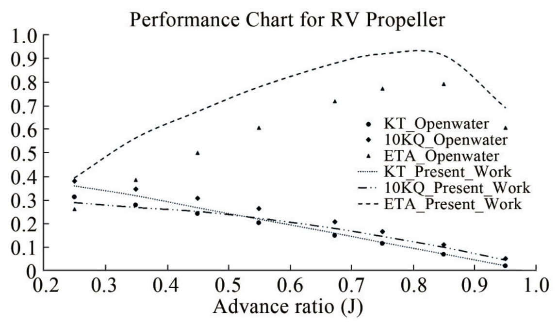Figure  13  Hydrodynamic performance of RV50 propeller

Download: Full-Size Img

The solver could predict the thrust coefficient with reasonable accuracy. Furthermore, as viscous effects were virtually applied in the solver, the torque coefficients were estimated with great errors. This condition results in the efficiency of predicting a greater value than that of the real condition. Figure 14 shows the rollup pattern of the RV50 propeller at a design advance ratio.

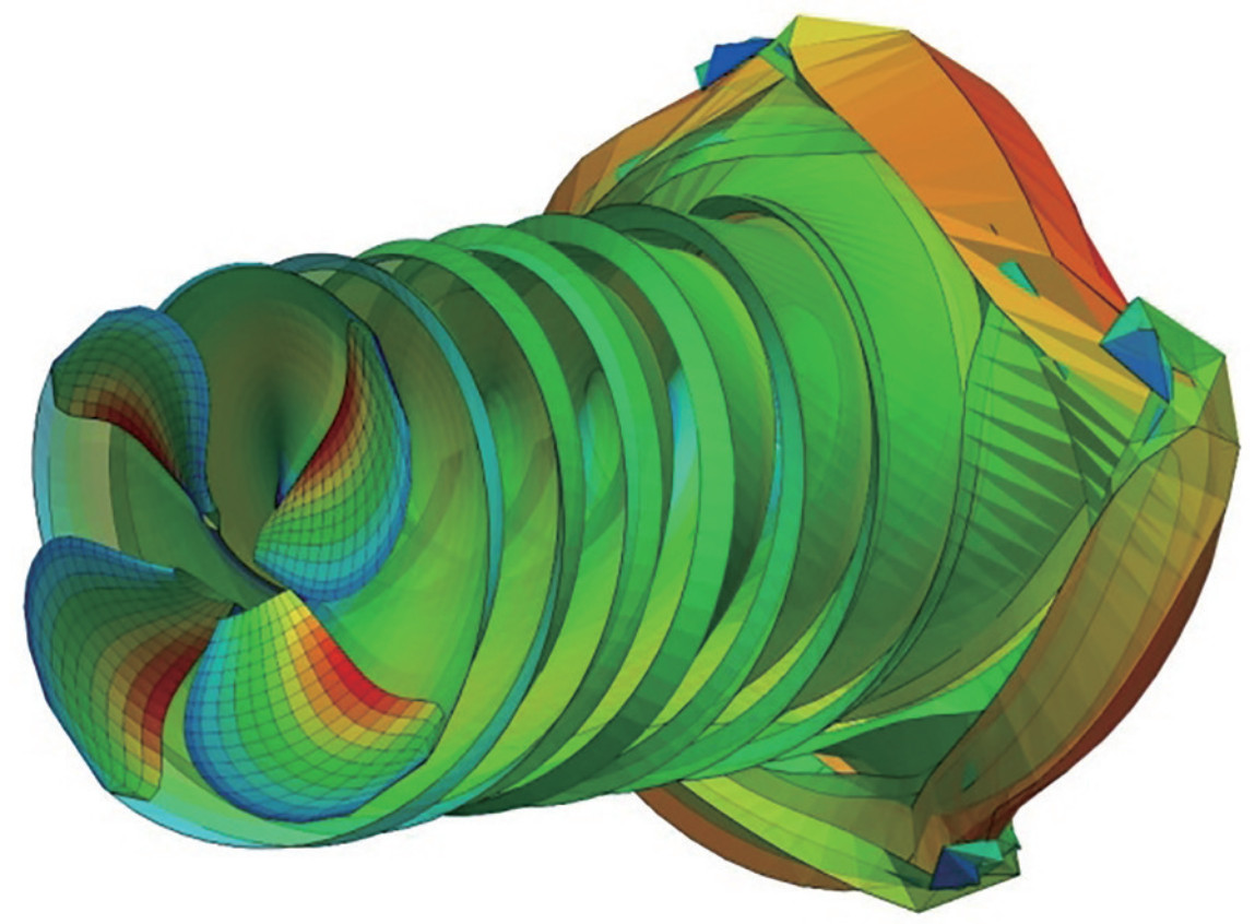Figure  14  Wake sheet pattern of the RV50 propeller at J = 0.623

Download: Full-Size Img

4   Coupling algorithm

After separately validating the solvers, they can be coupled to simulate the twin propeller behavior in the wake field of the RV50 hull. In the coupled solver, first, the fully appended hull was simulated in the NS solver until all the hydrodynamic variables (velocities and pressure field) became steady. Subsequently, the wake field behind the hull was used as the inlet velocity for the propeller in the BEM solver. To accomplish this task, the corresponding volumetric cell should be found (at each time step) for each surface panel for velocity matching. Figure 15 schematically shows the following algorithm.

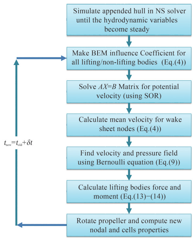Figure  15  Applied algorithm in the coupled solver

Download: Full-Size Img

5   Results and discussion

Based on the presented coupling algorithm, the simulation of the twin propellers of RV50 was simultaneously performed with both propellers, as shown in Figure 16. The propellers' direction of rotation was outward, which implies that the right propeller rotates clockwise, whereas the left propeller rotates counterclockwise.

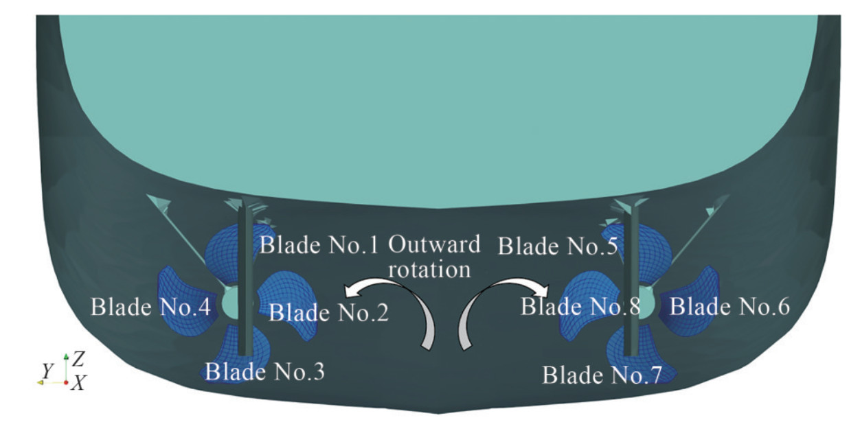Figure  16  Twin propeller of RV50

Download: Full-Size Img

The simulations were performed based on the design parameters (Table 5) on three different ship velocities. As shown in the table, the propeller rotational speed was calculated on its design advance ratio (J = 0.67 − 0.83).

At each velocity, the simulation was performed (based on the algorithm in Figure 15) until the propeller forces became steady. Figure 17 shows the time history of the left propeller force for the ship at a top speed (the right propeller force is almost the same, so its difference is not recognizable in this chart). Due to the completely transient nature of the BEM solver, the burst starting force appears in the chart in the early moments of the propeller rotation.

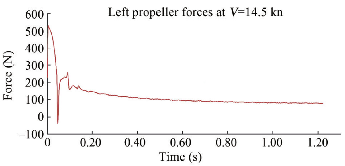Figure  17  Left propeller force at V = 14.5 kn

Download: Full-Size Img

Because each lifting body was separately modeled (Figure 16) in this study, the forces of each blade can be shown in a similar way (Figure 18).

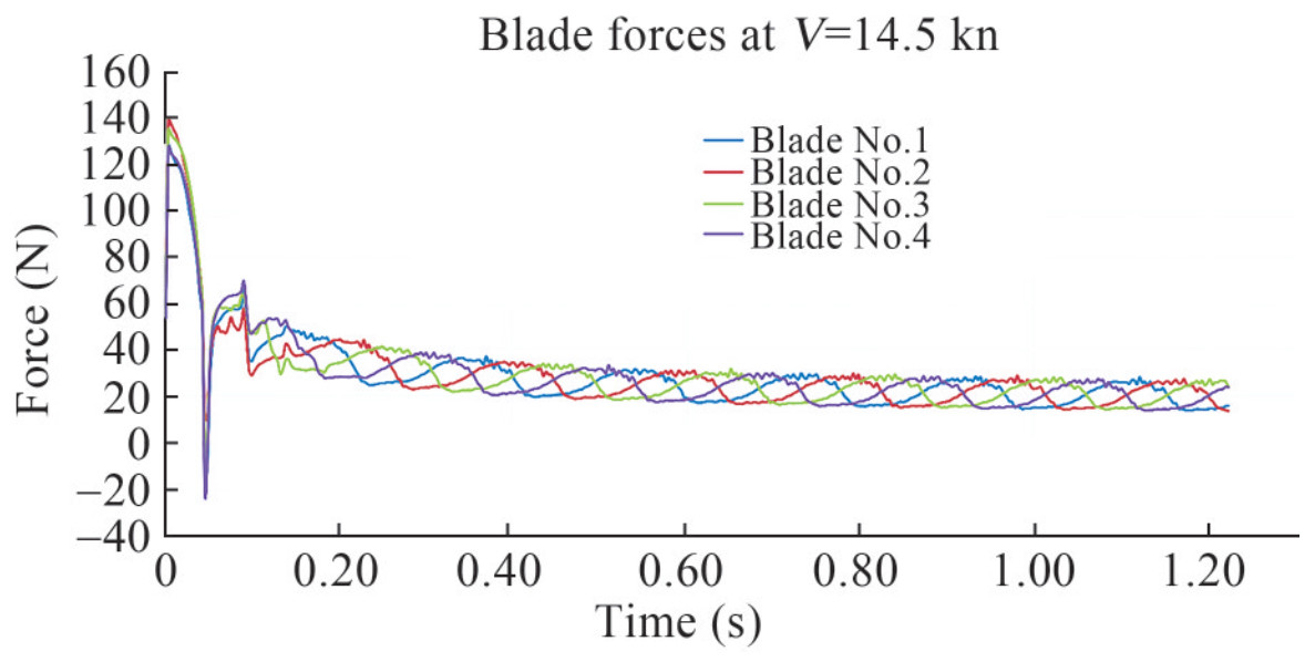Figure  18  Left propeller blade force at V = 14.5 kn

Download: Full-Size Img

As shown in Figure 18, each propeller force has a harmonic behavior, and this property is similar for opposite blades. Blades No. 1 and 3 or blades No. 2 and 4 are in opposite directions (Figure 16). The frequency of this harmonic behavior is almost the same as the propeller revolution (propellers rotate 4.3 rounds per second; see Table 5). Thus, the shaft bracket imposes a harmonic behavior on the blade force.

In the real self-propulsion test, at each specified velocity of the model, the propeller speed gradually increased until the net force on the carriage tended to zero. Table 5 shows the respective velocities for the ship and propeller extracted from the experiment. However, in the numerical self-propulsion (coupled solution in the present research), the fixed propeller speed was applied to the inviscid model, and as a result, the forces of the rotating disk were designated to the RANS model until the vessel's surge velocity converged to a steady value. Accordingly, the time history of balancing forces and ship velocity for n_p = 319.33 r/min (Table 5) is shown. As depicted in Figure 19, the total thrust for the twin propellers reached the vessel drag after almost 66 s. Accordingly, as shown in Figure 20, the vessel speed converged at 15.55 kn.

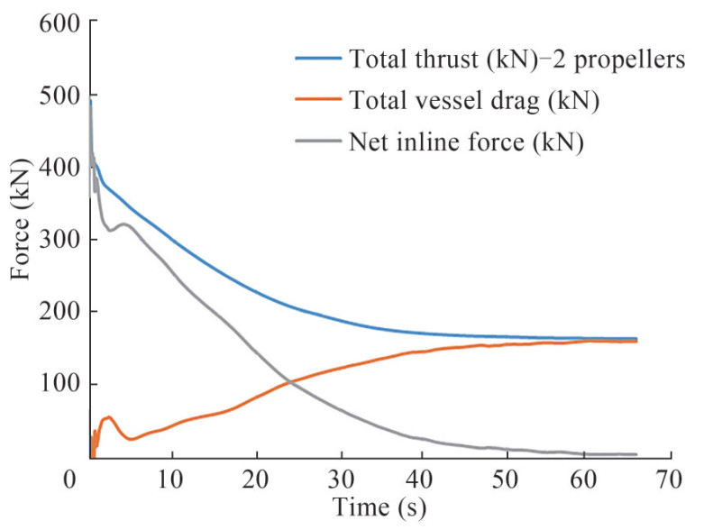Figure  19  Time history of the propeller thrust, ship total drag, and net balance force

Download: Full-Size Img

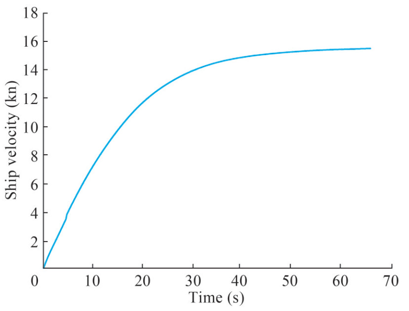Figure  20  Ship velocity increase in the computational self-propulsion until convergence

Download: Full-Size Img

The TSM was applied to capture the unsteady vortex sheet behind the propeller at each time step. Figure 21 shows the wake sheet of the propeller on three different time steps from the top view. Only the wake sheet pattern of blades No.2 and 8 (Figure 16) are shown for a good distinction.

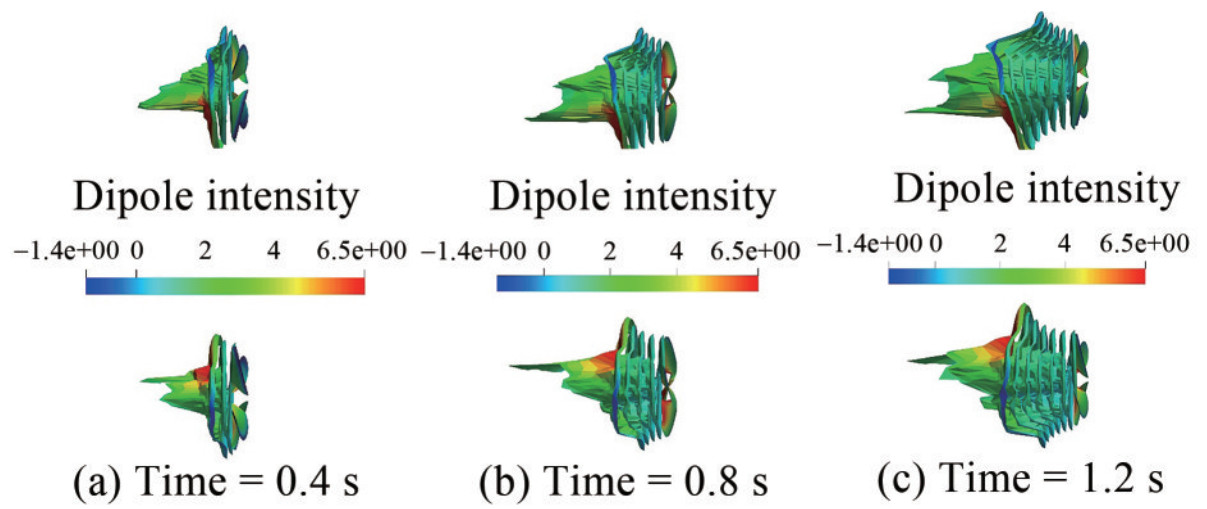Figure  21  Wake sheet pattern of blades Nos. 2 and 8 at V = 14.5 kn (Top view)

Download: Full-Size Img

Figure 22 shows the streamline of the left propeller from the top view. The 3D view of the propeller wake sheet pattern is also illustrated in Figure 23.

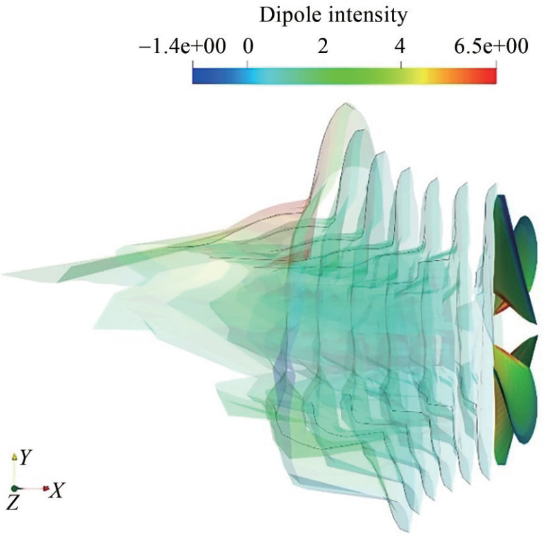Figure  22  Streamline of the wake sheet for the left propeller at V = 14.5 kn (top view; time = 1.2 s)

Download: Full-Size Img

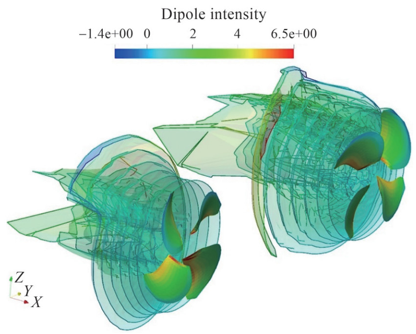Figure  23  3D view of the wake sheet pattern (blades No.2 and 8) at V = 14.5 kn (top view, time = 1.2 s)

Download: Full-Size Img

As a fully unstructured mesh was used, an asymmetrical wake field was produced, which led to different wake sheet patterns of the left and right propellers. Figure 24 shows the ship and propellers and the propeller wake sheet below the water surface.

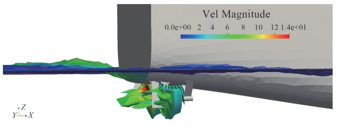Figure  24  Wake sheet below the free surface at V = 14.5 kn, time = 1.2 s

Download: Full-Size Img

By applying the solver on the presented test case at different velocities, based on Table 5, the thrust coefficient curve for the propeller behind the appended ship was achieved. Figure 25 compares the open water thrust coefficient with the fully appended ship results.

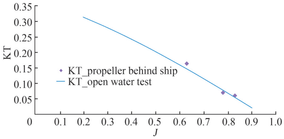Figure  25  Thrust coefficient in different flow conditions

Download: Full-Size Img

The results show that the propeller thrust in the open water test does not have much difference from the propeller thrust behind the RV50 hull. In fact, the average difference is $\frac{\mathrm{KT}_{\text {behind ship }}}{\mathrm{KT}_{\text {open water test }}} \cong 1.06$. Equation (31) defines the relative rotative efficiency η_r value and its range for rough estimations (Carlton 2018).

To get a good view of the subject, we consider the selfpropulsion test of the RV50, which was performed in Vienna Model Basin with the stock propeller No. 1090a4 as shown in Table 6 (RV50 Test Report 2011).

The thrust coefficient of propeller No. 1090a4 for the open water and self-propulsion tests is plotted in Figure 26. As shown, the thrust coefficients for the open water and self-propulsion tests are almost the same. Therefore, the computational results for a highly skewed propeller seem logical.

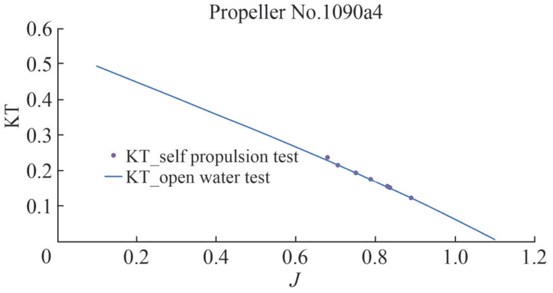Figure  26  Thrust coefficient for the propeller in the open water test and self-propulsion conditions

Download: Full-Size Img

This issue should be taken into consideration when the total propulsion power is estimated, especially in the concept design stage.

6   Conclusions

In the conceptual design of a ship propulsion system, there is tremendous demand for an efficient and accurate solver to predict the hydrodynamic performance of a propeller. In this research, a coupled viscous/inviscid solver was presented to calculate the hydrodynamic behavior of the twin propellers behind a fully appended ship. The inviscid solver is based on the potential flow, which is very efficient in calculating lifting body forces, such as propellers. An unsteady BEM was used to simulate the flows around the propeller. The TSM simulates the free wake rollup and its interaction at each time step. The BEM solver was validated by simulating a highly skewed propeller. The numerical results were compared with available data from the experimental open water test. The wake sheet pattern of the propeller when it encountered a uniform flow was also shown.

Moreover, an unsteady NS solver was used in combination with the VOF approach to capture the free surface. The moving mesh technique was also applied to simulate ship motions. To verify the RANS solver, the resistance of an oceanography research vessel in calm water at different velocities was investigated. The results were compared with a towing tank test results to validate the performance of the RANS solver.

Subsequently, the coupled RANS/BEM solver was used to simulate the twin propellers behind the RV50. In particular, the present study is not a real self-propulsion simulation because the effect of a propeller in disturbing the pressure field around a ship transom was not considered. For this reason, the calculated nominal wake was very low. Indeed, this approach may be called a quasi-self-propulsion because a virtual disk that represents the real propeller was implemented into the RANS solver. However, there is an interaction between the two solvers, as the propeller inflow wake computed in the RANS solver was fed into the unsteady BEM solver.

The proposed solver could simulate propeller thrusts with good accuracy. The solver could also show the wake sheet pattern of a propeller affected by the wake field velocity of the ship.

Nomenclature