Mechatronic Design and Maneuverability Analysis of a Novel Robotic Shark
https://doi.org/10.1007/s11804-022-00274-x
-
Abstract
In this paper, the mechatronic design and maneuverability analysis of a novel robotic shark are presented. To obtain good maneuverability, a barycenter regulating device is designed to assist the posture adjustment at low speeds. Based on the Newton-Euler approach, an analytical dynamic model is established with particular consideration of pectoral fins for three-dimensional motions. The hydrodynamic coefficients are computed using computational fluid dynamics (CFD) methods. Oscillation amplitudes and phases are determined by fitting an optimized fish body wave. The performance of the robotic shark is estimated by varying the oscillation frequency and offset angle. The results show that with oscillation frequency increasing, the swimming speed increases linearly. The robotic shark reaches the maximum swimming speed of 1.05 m/s with an oscillation frequency of 1.2 Hz. Furthermore, the turning radius decreases nonlinearly as the offset angle increased. The robotic shark reaches the minimum turning radius of 1.4 times the body length with 0.2 Hz frequency and 12° offset angle. In the vertical plane, as the pectoral fin angle increases, the diving velocity increases nonlinearly with increase rate slowing down.Article Highlights• The mechatronic design is presented for a novel robotic shark;• An analytical dynamic model is established with particular consideration of pectoral fins for three-dimensional motions;• Maneuverability analysis of the robotic shark is presented based on the established dynamic model. -
1 Introduction
Coral reefs are centers of marine biodiversity that host a large portion of marine life, which can provide irreplaceable economic and ecological functions including coastal protection, tourism and fisheries (Coker et al., 2014). With continuous expansion of human activities to the ocean, the population has decreased in recent years and the function of coral reef ecosystem declines gradually (Hughes et al., 2017; Moeller et al., 2021). Dynamic monitoring and understanding the coral reef system and related water environment such as temperature, dissolved oxygen and PH value is of great significance. Existing monitoring methods such as in-situ observation, ecological monitoring and remote sensing monitoring can't achieve close-up observation in a large range (Cai et al., 2019). As a novel biomimetic underwater vehicle, with excellent maneuverability and low noise, the robotic fish is good at the tasks mentioned above, especially for closeup observation.
In the past two decades, there is significant interest in developing various robotic fish maneuvering in BCF or MPF modes. Liu and Hu (2006) designed a robotic fish to realize fish-like swimming motions such as cruise-straight, cruisein-turn and ascent-decent. Chowdhury et al.(2011, 2014) designed a two-joint three-link robotic fish inspired by a carangiform fish aiming to investigate the swimming ability such as swimming speed and maneuverability. Yang et al. 2016) developed a robotic shark with an embedded vision system, which successfully realized flexible shark-like locomotion containing forward swimming, turning, diving, and surfacing. Inspired by the design of both fin-actuated robotic fish and buoyancy-driven gliding of underwater glider, Wang (2021) and Dong (2020) designed two different gliding fish robots which can swim flexibly and glide energy-efficiently in three dimensions. More about the investigations can refer to the recent review papers (Low, 2011; Raj, 2016; Yu et al., 2018; Duraisamy et al., 2019).
Most research work concerning the study of robotic fish are aiming at laboratory study such as investigations of new propulsion mechanisms, fins materials, maneuverability, control methods and so on. However, apart from the scientific interest paid to robotic fish, the applicative issues also deserve attention, such as watertight-cabin design, obstacle avoidance and disturbance rejection. Therefore, some researchers are beginning to explore the possibility of practical application of robotic fish. Zhang et al. (2016) designed a gliding robotic fish for autonomously sampling multiple water columns and related experiments were carried out in poor and in the Wintergreen Lake, Michigan. Wu et al. (2017) developed a gliding robotic dolphin capable of diving as deep as 300 meters. Also, laboratory and field experiments were conducted to demonstrate the effectiveness of the presented mechatronic design and control methods. Marcin et al. 2020) designed a biomimetic autonomous underwater vehicle for intelligence surveillance and reconnaissance and quantitatively studied noise generated by the vehicle for two different types of installed drives.
As a fundamental issue for analyzing the maneuverability of robotic fish, dynamic modeling has attracted a lot of attention. The most complicated and challenging problem of dynamic modeling lies in describing the hydrodynamics, especially for the thrust and hydrodynamic coefficients. Dynamic analysis modeling and data-driven modeling are two widely accepted methods. Wang and Tan (2013) developed a dynamic model for a tail-actuated robotic fish by merging rigid-body dynamics with Lighthill's large-amplitude elongated-body theory. Wang et al. (2018) formulated a complete three-dimensional dynamic model for the robotic fish actuated by pectoral and caudal fins based on quasi-steady hydrofoil theory. Considering the added mass effect, Du et al. 2019) established a dynamic model for a two-joint robotic fish. Due to the complexity of hydrodynamics, it is difficult to establish an accurate analytical model. Recently, data-driven modeling method emerges as a new method to solve the problem. Ren et al.(2013, 2015) established a data-based model through machine learning from real fish motion data. Verma and Xu (2016) proposed a novel data-assisted dynamical model for speed control, in which data of pulse and step responses were collected from designated experimental trials. Yu et al. (2016) established a data-driven dynamic modeling method for multi-joint robotic fish, in which experimental data of the swimming were collected to identify the parameters directly.
In this paper, due to the convenience of the internal equipment arrangement and excellent static stability, a three-joint robotic shark is developed by mimicking the shape of a shark. Both the mechatronic design and three-dimensional maneuverability analysis are illustrated. Especially, the added mass of each joint is obtained by numerical simulation rather than approximation technique. Based on the dynamic model, swimming speed in different motion parameters and threedimensional spiral motion in different cases are simulated.
2 Mechatronic design
Based on its powerful caudal fin and attached muscles, great white sharks can obtain high-speed and good-maneuverability swimming performance easily. However, limited by the level of engineering materials, it is difficult to find a flexible material that can generate enough power to replicate the motion of sharks. Ignoring the bionic structure and inheriting these advantages in bionic propulsion mode, a robotic shark is designed by mimicking a real great white shark. Figure 1 shows the mechanical design of a novel robotic shark for coral reef detection. The hull design is inspired by the shape of a great white shark because of its cylindrical-like shape. The shape feature allows the robot shark to carry more equipments and has better static stability. The use of waterproof connector makes it more suitable for practical application. The robotic shark is about 1.23 m long and weighs about 8.2 kg. Table 1 shows the basic parameters of the robotic shark.
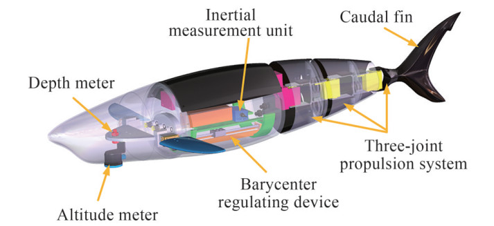 Figure 1 The detailed mechanical configuration of the robotic sharkTable 1 Technical characteristics of the robotic shark
Items Characteristics Dimensions (m)
(L × W × H)~1.23×0.82×0.33 Total mass (kg) ~8.2 Number of joints 3 Driving system Servo motor Sensors 9-DOF IMU, Depth meter, Altitude meter Power supply 14.8 V 5 200 mAh rechargeable Li-Po battery The robotic shark is mainly divided into four parts, a threejoint propulsion system, a barycenter regulating device, a control cabinet, a sensory cabinet. The three-joint propulsion system is the main source of power for propulsion. Three waterproof servo motors are used to drive the three joints. A rigid structure made of aluminum alloy is used to connect adjacent servo motors. In order to ensure good hydrodynamic performance of the three-joint propulsion system, a shell made of photosensitive resin is installed in each joint. In addition, the design of the tail fin is entirely based on the shark's caudal fin and made of photosensitive resin. By adjusting the motion parameters such as frequency, amplitude and offset angles, different swimming modes can be obtained.
A barycenter regulating device is designed to enhance the mobility of vertical motion in low speed by adjusting center of gravity. The mechatronic design of barycenter regulating device is shown in Figure 2. The device is mainly composed of a stepping motor, a lead screw, a movable weight and a bracket. By adjusting the position of the movable weight, center of gravity of the robotic shark can be adjusted.
 Figure 2 The detailed mechanical configuration of barycenter regulating device
In order to ensure sufficient compressive strength, the control cabinet is made of aluminum alloy. Also, O-rings are selected to keep the cabin waterproof. The control cabinet mainly holds a Stm32 controller, a Li-Po battery and an inertial measurement unit (IMU) for attitude perception.
The sensory cabinet mainly holds an altitude meter and a depth meter for position information acquisition in the vertical plane. Besides, adequate space is reserved for water quality monitoring sensors on the back of the robotic shark. The sensor cabinet is also made of photosensitive resin.
3 Kinematics and dynamics
3.1 Kinematics
In order to describe the kinematic and dynamic characters of the robotic shark in six degrees of freedom (DOF), as shown in Figure 3, two coordinates are established, i.e., an earth-fixed reference frame $C_{n}=o_{n} x_{n} y_{n} z_{n}$ and a body-fixed reference frame $C_{g}=o_{g} x_{g} y_{g} z_{g}$. Also, the origin of bodyfixed reference frame is fixed at the center of gravity. The position vector $\boldsymbol{\eta}_{1}=[x, y, z]^{\mathrm{T}}$ and orientation vector $\boldsymbol{\eta}_{2}=[\varphi, \theta, \psi]^{\mathrm{T}}$ of the robotic shark is described in the earthfixed reference frame. The linear velocity vector $\boldsymbol{v}_{1}=$ $[u, v, w]^{\mathrm{T}}$ and angular velocity $\boldsymbol{v}_{2}=[p, q, r]^{\mathrm{T}}$ are defined in the body-fixed reference frame. $\boldsymbol{\tau}_{1}=[X, Y, Z]^{\mathrm{T}}$ and $\boldsymbol{\tau}_{2}=$ $[K, M, N]^{\mathrm{T}}$ describe respectively the forces and moments acting on the robotic shark in the body-fixed reference frame.
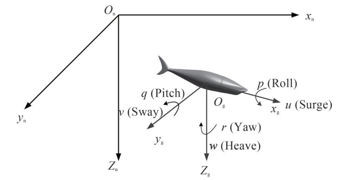 Figure 3 Schematic illustration of two coordinate frames
According to Fossen (2011), the first-order derivative of the position vector and orientation vector in the earth-fixed reference frame can be transformed from the linear velocity vector and angular velocity vector in the body-fixed reference frame. The relationship can be described as,
$$ \left\{\begin{array}{l} \dot{\boldsymbol{\eta}}_{1}=J_{1}\left(\boldsymbol{\eta}_{2}\right) \boldsymbol{v}_{1} \\ \dot{\boldsymbol{\eta}}_{2}=J_{2}\left(\boldsymbol{\eta}_{2}\right) \boldsymbol{v}_{2} \end{array}\right. $$ (1) Here, J1 and J2 represent the Euler transformation matrices, which can be expressed as follows. To simplify the expression, c·= cos (·), s·= sin (·), t·= tan (·).
$$ \boldsymbol{J}_{1}\left(\boldsymbol{\eta}_{2}\right)=\left[\begin{array}{ccc} \mathrm{c} \psi \mathrm{c} \theta & -\mathrm{s} \psi \mathrm{c} \varphi+\mathrm{c} \psi \mathrm{s} \theta \mathrm{s} \varphi & \mathrm{s} \psi \mathrm{s} \varphi+\mathrm{c} \psi \mathrm{c} \varphi \mathrm{s} \theta \\ \mathrm{s} \psi \mathrm{c} \theta & \mathrm{c} \psi \mathrm{c} \varphi+\mathrm{s} \varphi \mathrm{s} \theta \mathrm{s} \psi & -\mathrm{c} \psi \mathrm{s} \varphi+\mathrm{s} \theta \mathrm{s} \psi \mathrm{c} \varphi \\ -\mathrm{s} \theta & \mathrm{c} \theta \mathrm{s} \varphi & \mathrm{c} \theta \mathrm{c} \varphi \end{array}\right] $$ (2) $$ \boldsymbol{J}_{2}\left(\boldsymbol{\eta}_{2}\right)=\left[\begin{array}{ccc} 1 & \mathrm{~s} \varphi \mathrm{t} \theta & \mathrm{c} \varphi \mathrm{t} \theta \\ 0 & \mathrm{c} \varphi & -\mathrm{s} \varphi \\ 0 & \mathrm{~s} \varphi / \mathrm{c} \theta & \mathrm{c} \varphi / \mathrm{c} \theta \end{array}\right] $$ (3) 3.2 Dynamics
The equations of motion related to 6 DOF dynamics of the robotic shark can be written as,
$$ \boldsymbol{M} \dot{\boldsymbol{v}}+\boldsymbol{C}(\boldsymbol{v})\boldsymbol{v}+\boldsymbol{D}(\boldsymbol{v})\boldsymbol{v}+\boldsymbol{g}(\boldsymbol{\eta})=\boldsymbol{\tau} $$ (4) where $\boldsymbol{v}=\left[\boldsymbol{v}_{1}^{\mathrm{T}}, \boldsymbol{v}_{2}^{\mathrm{T}}\right]^{\mathrm{T}}, \boldsymbol{M}=\boldsymbol{M}_{R B}+\boldsymbol{M}_{A}, \boldsymbol{C}(\boldsymbol{v})=\boldsymbol{C}_{R B}(\boldsymbol{v})+$ $\boldsymbol{C}_{A}(\boldsymbol{v}), \boldsymbol{D}(\boldsymbol{v})=\boldsymbol{D}_{l}+\boldsymbol{D}_{n}(\boldsymbol{v}) . \boldsymbol{M}_{R B}, \boldsymbol{C}_{R B}(\boldsymbol{v})$ are mass-inertia matrix and coriolis-centripetal matrix related to rigid body. Also, $\boldsymbol{M}_{A}$ and $\boldsymbol{C}_{A}(\boldsymbol{v})$ are mass-inertia matrix and corioliscentripetal matrix related to added mass. $\boldsymbol{D}_{1}$ is the linear damping matrix and $\boldsymbol{D}_{n}(\boldsymbol{v})$ is the nonlinear damping matrix. $\boldsymbol{g}(\boldsymbol{\eta})$ is the restoring forces and moments in the body-fixed reference system.
In order to simplify the dynamic model, several assumptions are made.
1) The robotic shark moves at low speed, nonlinear and coupled.
2) The robotic shark has several symmetry planes so that the off-diagonal elements in the added mass matrix can be neglected.
Based on the assumptions mentioned above, the relative matrices in the dynamic model can be written as,
$$ \boldsymbol{M}_{R B}=\left[\begin{array}{cccccc} m & 0 & 0 & 0 & 0 & 0 \\ 0 & m & 0 & 0 & 0 & 0 \\ 0 & 0 & m & 0 & 0 & 0 \\ 0 & 0 & 0 & I_{x} & 0 & 0 \\ 0 & 0 & 0 & 0 & I_{y} & 0 \\ 0 & 0 & 0 & 0 & 0 & I_{z} \end{array}\right] $$ (5) $$ \boldsymbol{M}_{A}=\left[\begin{array}{cccccc} X_{\dot{u}} & 0 & 0 & 0 & 0 & 0 \\ 0 & Y_{\dot{v}} & 0 & 0 & 0 & 0 \\ 0 & 0 & Z_{\dot{w}} & 0 & 0 & 0 \\ 0 & 0 & 0 & K_{\dot{p}} & 0 & 0 \\ 0 & 0 & 0 & 0 & M_{\dot{q}} & 0 \\ 0 & 0 & 0 & 0 & 0 & N_{\dot{r}} \end{array}\right] $$ (6) $$ \boldsymbol{C}_{R B}(\boldsymbol{v})=\left[\begin{array}{cccccc} 0 & 0 & 0 & 0 & m w & -m v \\ 0 & 0 & 0 & -m w & 0 & m u \\ 0 & 0 & 0 & m v & -m u & 0 \\ 0 & m w & -m v & 0 & I_{z} r & -I_{y} q \\ -m w & 0 & m u & -I_{z} r & 0 & I_{x} p \\ m v & -m u & 0 & I_{y} q & -I_{x} p & 0 \end{array}\right] $$ (7) $$ \boldsymbol{C}_{A}(\boldsymbol{v})=\left[\begin{array}{cccccc} 0 & 0 & 0 & 0 & -Z_{\dot{w}} w & Y_{\dot{v}} v \\ 0 & 0 & 0 & Z_{\dot{w}} w & 0 & -X_{\dot{u}} u \\ 0 & 0 & 0 & -Y_{\dot{v}} v & X_{\dot{u}} u & 0 \\ 0 & -Z_{\dot{w}} w & Y_{\dot{v}} v & 0 & -N_{\dot{r}} r & M_{\dot{q}} q \\ Z_{\dot{w}} w & 0 & -X_{\dot{i}} u & N_{\dot{r}} r & 0 & -K_{\dot{p}} p \\ -Y_{\dot{v}} v & X_{\dot{i}} u & 0 & -M_{\dot{q}} q & K_{\dot{p}} p & 0 \end{array}\right] $$ (8) $$ \boldsymbol{D}_{l}=\left[\begin{array}{cccccc} X_{u} & 0 & 0 & 0 & 0 & 0 \\ 0 & Y_{v} & 0 & 0 & 0 & 0 \\ 0 & 0 & Z_{w} & 0 & 0 & 0 \\ 0 & 0 & 0 & K_{p} & 0 & 0 \\ 0 & 0 & 0 & 0 & M_{q} & 0 \\ 0 & 0 & 0 & 0 & 0 & N_{r} \end{array}\right] $$ (9) $$ \boldsymbol{D}_{n}(\boldsymbol{v})=\left[\begin{array}{cccccc} X_{u|u|}|u| & 0 & 0 & 0 & 0 & 0 \\ 0 & Y_{v|v|}|v| & 0 & 0 & 0 & 0 \\ 0 & 0 & Z_{w|w|}|w| & 0 & 0 & 0 \\ 0 & 0 & 0 & K_{p|p|}|p| & 0 & 0 \\ 0 & 0 & 0 & 0 & M_{q|q|}|q| & 0 \\ 0 & 0 & 0 & 0 & 0 & N_{r|r|}|r| \end{array}\right] $$ (10) $$ \boldsymbol{g}(\boldsymbol{\eta})=\left[\begin{array}{c} 0 \\ 0 \\ 0 \\ \left(z_{g} W-z_{b} B\right) \cos \theta \sin \phi \\ \left(z_{g} W-z_{b} B\right) \sin \theta \\ 0 \end{array}\right] $$ (11) The dynamic model of the robotic shark can be simplified as,
$$ \dot{u}=\frac{\left(Z_{\dot{w}}-m\right) w q+\left(m-Y_{\dot{v}}\right) v r-X_{u} u-\left.X_{u \mid u}\right|^{u}|u|+X}{m-X_{\dot{u}}} $$ (12) $$ \dot{v}=\frac{\left(m-Z_{\dot{w}}\right) w p+\left(X_{\dot{u}}-m\right) u r-Y_{v} v-Y_{v|v|} v|v|+Y}{m-Y_{\dot{v}}} $$ (13) $$ \dot{w}=\frac{\left(Y_{\dot{v}}-m\right) v p+\left(m-X_{\dot{u}}\right) u q-Z_{w} w-Z_{w|w|} w|w|+Z}{m-Z_{\dot{w}}} $$ (14) $$ \begin{aligned} &\dot{p}=\frac{\left(Z_{\dot{w}}-Y_{\dot{v}}\right) w v+\left(I_{y}+N_{\dot{r}}-I_{z}-M_{\dot{q}}\right) q r-K_{p} p-K_{p|p|} p|p|}{I_{x}-K_{\dot{p}}} \\ &+\frac{-\left(z_{g} W-z_{b} B\right) \cos \theta \sin \varphi+K}{I_{x}-K_{\dot{p}}} \end{aligned} $$ (15) $$ \begin{aligned} &\dot{q}=\frac{\left(X_{\dot{u}}-Z_{\dot{w}}\right) u w+\left(I_{z}-I_{x}+K_{\dot{p}}-N_{\dot{r}}\right) p r-M_{q} q-M_{q|q|} q|q|}{I_{y}-M_{\dot{q}}} \\ &+\frac{-\left(z_{g} W-z_{b} B\right) \sin \theta+M}{I_{y}-M_{\dot{q}}} \end{aligned} $$ (16) $$ \dot{r}=\frac{\left(Y_{\dot{v}}-X_{\dot{u}}\right) u v+\left(I_{x}-I_{y}+M_{\dot{q}}-K_{\dot{p}}\right) p q-N_{r} r-N_{r|r|} r|r|+N}{I_{z}-N_{\dot{r}}} $$ (17) 3.3 Hydrodynamic analysis
Neglecting the hydrodynamic force induced by trailing edge vortex, the force acting on each joint and caudal fin is caused by oscillatory acceleration of the joint. According to Lighthill (1971), the relationship can be expressed as,
$$ F_{c i}=\int_{0}^{l_{i}}-A_{c i} \ddot{\alpha}_{i}\left(\sigma_{i}\right) \hat{\boldsymbol{w}}_{i} \mathrm{~d} \sigma_{i} $$ (18) Here, Aci is the added mass of the ith joint caused by transverse acceleration. αi is instantaneous turning angle of each joint. $\hat{\boldsymbol{w}}_{i}$ is a unit vector perpendicular to the spinal column. Fci is the force acting vertically on each joint.
Based on the force acting vertically on each joint, the total forces and moments acting on the rigid body can be defined as,
$$ X_{c}=\sum\limits_{i=1}^{3} F_{c i} \sin \left(\theta_{c i}\right) $$ (19) $$ Y_{c}=\sum\limits_{i=1}^{3} F_{c i} \cos \left(\theta_{c i}\right) $$ (20) $$ N_{c}=\sum\limits_{i=1}^{3} x_{i}^{c} F_{c i} \cos \left(\theta_{c i}\right)+\sum\limits_{i=1}^{3} y_{i}^{c} F_{c i} \sin \left(\theta_{c i}\right) $$ (21) Here, θci is the angle between the joint and the x-axis in the body-fixed reference frame. xic and yic are distance between the center point of force acting on each joint and the origin of coordinates along x-axis and y-axis in the body-fixed reference frame, respectively. Here, we assume that the center point of force is at the geometric center of each joint.
Also, the force acting on each pectoral fin can be written as,
$$ F_{L i}=\frac{1}{2} \rho s_{p i} v_{p i}^{2} C_{L i} $$ (22) $$ F_{D i}=\frac{1}{2} \rho s_{p i} v_{p i}^{2} C_{D i} $$ (23) Here, FLi is lift force and FDi represents drag force. CLi and CDi are lift coefficient and drag coefficient, respectively. spi is the surface area of the pectoral fin. ρ is the density of water, 998 kg/m3.
The total force and moment of pectoral fins acting on the rigid body can be defined as,
$$ X_{p}=\sum\limits_{i=1}^{2} F_{D i} $$ (24) $$ Z_{p}=\sum\limits_{i=1}^{2} F_{L i} $$ (25) $$ K_{p}=\sum\limits_{i=1}^{2} F_{L i} y_{i}^{p} $$ (26) $$ M_{p}=\sum\limits_{i=1}^{2}\left(F_{L i} x_{i}^{p}+F_{D i} z_{i}^{p}\right) $$ (27) $$ N_{r}=\sum\limits_{i=1}^{2} F_{D i} y_{i}^{p} $$ (28) where xip, yip and zip are distance between the center point acting on each pectoral fin and the origin of coordinates along x-axis, y-axis and z-axis respectively in the body-fixed reference frame.
3.4 Parameter identification
In order to effectively evaluate the motion performance of robotic shark, the relevant parameters need to be identified such as added mass, damping coefficients and so on. In this work, two main methods are used. One is based on HessSmith method, which is used for calculating the added mass. The other method is based on Computational Fluid Dynamics (CFD), which is used for estimate the damping coefficients and hydrodynamic coefficients acting on pectoral fins.
First, based on Hess-Smith method and CFD method, neglecting the effects of pectoral fins, the added mass and damping coefficients are calculated. The results are shown in table 2.
Table 2 Hydrodynamic coefficients and mass properties of the robotic sharkItem Value Item Value $X_{\dot{u}}$(kg) 1.68 Xu|u|(kg/m) -2.26 $Y_{\dot{v}}$(kg) 21.78 Yv|v|(kg/m) -13.04 $Z_{\dot{w}}$(kg) 21.40 Zw|w|(kg/m) -22.33 $K_{\dot{p}}$(kg·m2) 0.005 5 Nr|r|(kg·m2) -0.52 $M_{\dot{q}}$(kg·m2) 0.77 Ix(kg·m2) 0.075 $N_{\dot{r}}$(kg·m2) 1.16 Iy(kg·m2) 0.48 Xu(kg/s) -0.24 Iz(kg·m2) 0.47 Yv(kg/s) -41.98 Ac1(kg·m2) 1.83 Zw(kg/s) -15.78 Ac2(kg·m2) 1.37 Nr(kg·m2/s) -10.53 Ac3(kg·m2) 0.87 The solver adopted in CFD simulations is the STARCCM+ 12.02, using the finite volume, viscous and incompressible unsteady RANS equations. The k-ω shear stress transport (SST) turbulence model is employed owing to its good prediction capability with reasonable computational cost (Gao et al., 2018). As shown in Figure 4, the size of the domain is 10.4 m×5.2 m×5.2 m. The length is eight times the length of the robotic shark. A dimensionless wall distance y + is defined to express thickness for the volume mesh adjacent to the body surface, which is given as $y^{+}=y \sqrt{\rho \tau_{\omega}} / \mu $, ρ is the fluid density, μ is the fluid dynamic viscosity, y is the mesh node distance to wall, τω is the wall shear stress.
$$ y=\sqrt{80} L y^{+} R e^{-\frac{13}{14}} $$ (29) 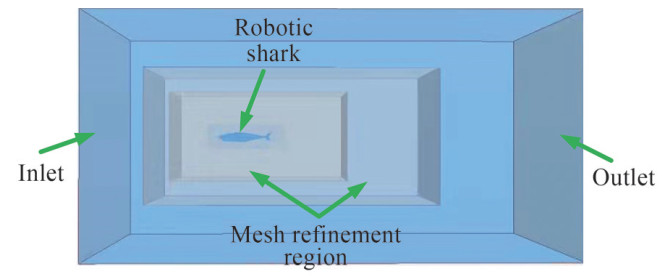 Figure 4 Schematic of computional domain for robotic shark
where Re is the Reynolds number, L is the characteristic length.
The number of grids will directly affect the numerical solution results. In order to verify that the numerical solution results of robotic shark are independent of the grids, the resistance of robotic shark along the x-axis direction are numerically simulated with different y+ values. The results are shown in table 3. It can be seen that when the average y+ is 32, the computational value remains stable. To ensure simulation accuracy and reduce computation costs, the grid size of 1.69 million is adopted.
Table 3 Computational values with different y+Mesh size (million cells) Average y+ value Computational value (N) 4.61 20.9 1.09 1.69 32 1.09 0.62 44.8 1.12 0.24 66.8 1.19 Then, the hydrodynamic coefficients CpiL and CpiD of pectoral fins is determined using Computational Fluid Dynamics (CFD) method. According to previous results, the hydrodynamic coefficients could be simplified as a function of the angle of attack, e.g., quadratic polynomial for a drag coefficient and monomial for lift coefficient. As shown in Figure 4, the computational domain is a cuboid. The size of the domain is 2 m×1.2 m×1.2 m. The length is five times the length of chord length. The boundary conditions on each side of the region are as follows. At the left boundary, a uniform velocity is prescribed. At the four side-walls, symmetryplane boundary conditions are applied. At the right boundary, a pressure-outlet boundary condition is used. The incoming flow velocity is set to be 1 m/s. To simplify the simulation, overlapping grid method is used. The overlapping region is shown in Figure 5.
 Figure 5 Schematic of computional domain for pectoral fin
Also, the polyhedral mesh is adopted and the mesh of the surface of the pectoral fin is shown in Figure 6. The hydrodynamic coefficients of pectoral fin are fitted as follows:
$$ C_{L i}=2.022 \alpha_{p i}-0.198 $$ (30) $$ C_{D i}=1.125 \alpha_{p i}^{2}-0.328 \alpha_{p i}+0.074 $$ (31) 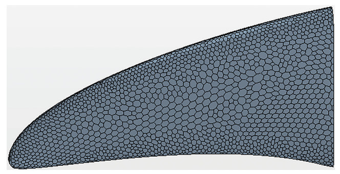 Figure 6 Mesh of the surface of pectoral fin
where αpi represents the angle of pectoral fin.
4 Numerical simulation
4.1 Motion of propulsion system
As shown in Figure 7, the rhythmic movement of each joint can be expressed as
$$ \left\{\begin{array}{l} \alpha_{1}(t)=\alpha_{01}+\alpha_{A 1} \sin \left(2 \pi f_{1} t\right) \\ \alpha_{2}(t)=\alpha_{02}+\alpha_{A 2} \sin \left(2 \pi f_{2} t+\varphi_{21}\right) \\ \alpha_{3}(t)=\alpha_{03}+\alpha_{A 3} \sin \left(2 \pi f_{3} t+\varphi_{32}\right) \end{array}\right. $$ (32) 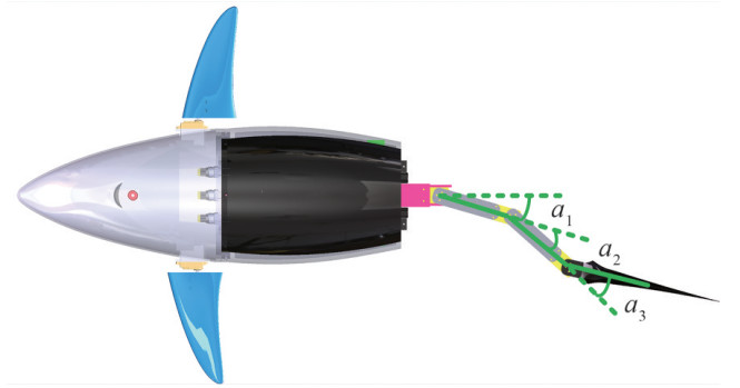 Figure 7 Instantaneous angle of each joint
Here, αi is instantaneous angle of the ith joint. fi and αAi are oscillating frequency and amplitude. α0i is the bias of beating. φ21 and φ32 are phase lags between adjacent joints.
According to our previous work (Gao et al., 2021), based on the optimized parameters, some parameters are determined by fitting the fish body wave. As a result, the motion of each joint follows the sinusoidal law.
$$ \left\{\begin{array}{l} \alpha_{1}(t)=\alpha_{01}+8.5 \sin \left(2 \pi f_{1} t\right) \\ \alpha_{2}(t)=\alpha_{02}+23.17 \sin \left(2 \pi f_{2} t-0.802\right) \\ \alpha_{3}(t)=\alpha_{03}+29.27 \sin \left(2 \pi f_{3} t-1.978\right) \end{array}\right. $$ (33) In the following work, the performance of the robotic shark is estimated by varying the frequency and offset angle.
4.2 Swimming speeds in different cases
In order to estimate the performance of the robotic shark, swimming speeds at different oscillation parameters are first simulated based on the dynamic model established in the last section. To simplify the parameters, the oscillation frequency and offset angle of each joint keep the same. By varying the oscillation frequency and offset angle, different swimming speeds are achieved.
Figure 8 shows the instantaneous swimming speeds at different oscillation frequencies with offset angle 0°. It can be seen that under the action of thrust, swimming speed increases gradually and then keeps periodic oscillation due to the periodic oscillations of propulsion system. Also, with the increase of oscillation frequency, swimming speed increases and the time to reach the maximum value is reduced. Considering the constraints of the driving motor, the maximum oscillation frequency is set to 1.2 Hz. In this case, the robotic shark reaches the maximum swimming speed of 1.05 m/s. The time to reach the maximum swimming speed is about 10 s.
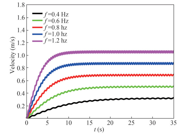 Figure 8 Instantaneous swimming speeds for five oscillation frequencies
Figure 9 shows the average swimming speed at different oscillation frequencies for five offset angles. Considering the geometric constraints of robotic shark, the maximum offset angle of each joint is about 12°. It can be seen that, with the oscillation frequency increasing, the swimming speed increases linearly. Also, although the offset angle has a negative effect on swimming speed, it has smaller effect than oscillation frequency.
 Figure 9 Swimming speeds at different frequencies for five offset angles
4.3 Turning radiuses in different cases
To estimate the turning performance of the robotic shark, turning radiuses and angular velocities at different oscillation frequencies and offset angles are simulated.
As shown in Figure 10, different turning radiuses are achieved by varying oscillation frequency and offset angle. It can be seen that with the increase of offset angle, turning radius decreases nonlinearly. When the offset angle starts to increase, turning radius of the robotic shark decreases rapidly. As the offset angle continues to increase, the change of turning radius gradually moderates. Also, it can be seen that the turning radius decreases with the oscillation frequency decreasing. Therefore, to obtain a small turning radius, it is important to control both the oscillation frequency and offset angle. Among all cases studied, the minimum turning radius is achieved with 0.2 Hz frequency and 12° offset angle, which is about 1.4 times the body length.
 Figure 10 Turning radius at different offset angles for four oscillation frequencies
Figure 11 shows the angular velocities at different oscillation frequencies and offset angles. Angular velocity increases with oscillation frequency and offset angle increasing. Combined with Figure 8, in the case of offset angle 12°, it can be seen that with oscillation frequency increasing, the angular speed greatly increases while the turning radius changes slightly. Therefore, the heading angle can be changed quickly through high oscillation frequency and large offset angle.
 Figure 11 Angular velocities at different offset angles for four oscillation frequencies
4.4 Motion characteristics in the vertical plane
In order to analyze the motion characteristics in the vertical plane, diving velocities at different oscillation frequencies and pectoral fin angles are first simulated. It should be noted that the rotation about x axis and y axis are neglected. In all cases, the offset angle keeps 0°.
As shown in Figure 12, different diving velocities are achieved by varying oscillation frequency and pectoral fin angles. It can be seen that with the increase of pectoral fin angle, diving velocity increases nonlinearly. As the pectoral fin angle increases, the increase rate of diving velocity slows down. One reason is that larger pectoral angle leads to larger resistance, which will reduce the swimming speed at the final steady state. Also, it can be seen that diving velocity increases linearly as the oscillation frequency increases. Among all cases studied, the maximum diving velocity is achieved with frequency 0.8 Hz and pectoral fin angle 30°, which is about 0.19 m/s.
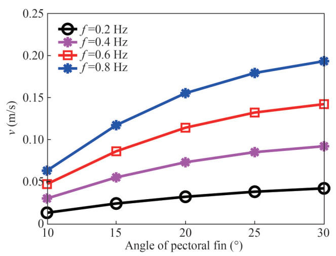 Figure 12 Diving velocities at different pectoral fin angles for four oscillation frequencies
To further analyze the motion characteristic in three-dimensional space, simulation of spiral descent is carried out based on the dynamic model. Initially, the robotic shark keeps static with zero attitude and velocity. The angle of the pectoral fins keeps 30° in the whole simulation. As a result, the robotic shark begins to swim forward and dive. The oscillation frequency and offset angle are set to be 0.5 Hz and 10°, respectively.
The three dimensional path and motion states of the robotic shark in spiral motion are shown in Figures 13 and 14, respectively. It can be seen that driven by the three-joint propulsion system, the robotic shark begins to accelerate. At t=20 s, the robotic shark reaches the maximum speed, about 0.23 m/s and then keeps steady. As the velocity of the robotic shark increases, the lift force generated by pectoral fins also increases gradually. As a result, the velocity of diving firstly increases and finally reaches a stable state. Under the action of pectoral fins, diving velocity of the robotic shark is approximately 0.09 m/s.
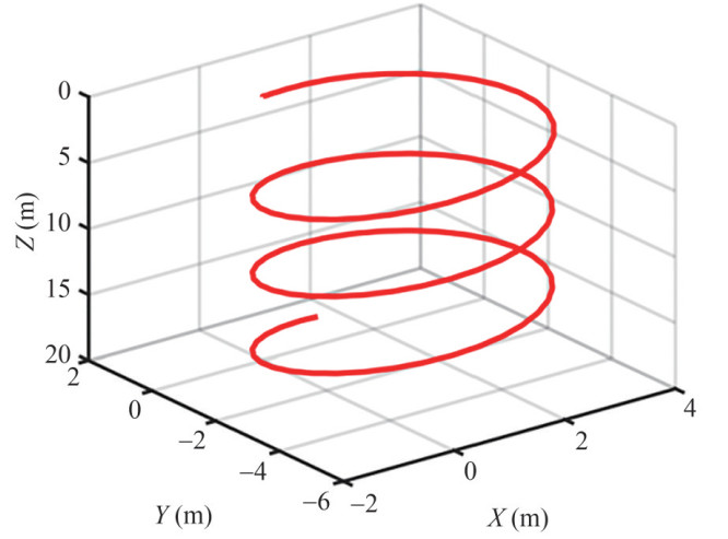 Figure 13 Three dimensional path of the spiral motion
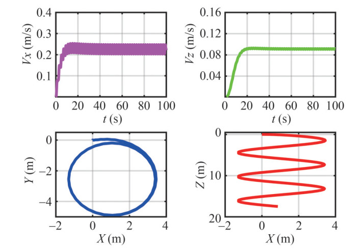 Figure 14 Motion states of the robotic shark in spiral motion
5 Conclusions
In this work, mechatronic design and maneuverability analysis of a novel robotic shark for coral reef detection is presented. Dynamic model is established based on NewtonEuler method. Based on the dynamic model, swimming speeds in different oscillation parameters and spiral motion based on pectoral fins are conducted to further analyze the performance of the robotic shark. The results suggest the following conclusions,
(1) With oscillation frequency increasing, swimming speed increases linearly. The robotic shark reaches the maximum swimming speed of 1.05 m/s when the oscillation frequency is 1.2 Hz.
(2) With offset angle increasing, turning radius decreases nonlinearly. The robotic shark reaches the minimum turning radius of 1.4 times body length with frequency 0.2 Hz and offset angle 12°.
(3) As pectoral fin angle increases, diving velocity increases nonlinearly with increase rate slowing down. The robotic shark reaches the maximum diving speed of 0.19 m/s with frequency 0.8 Hz and pectoral fin angle 30°.
In future work, a real robotic shark will be made as designed. Also, we will continue to build a more accurate dynamic model by taking full account of the influence of barycenter regulating device and variations in hydrodynamic parameters. Finally, experiments will be done to further modify the dynamic model.
-
Figure 1 The detailed mechanical configuration of the robotic shark
Figure 2 The detailed mechanical configuration of barycenter regulating device
Figure 3 Schematic illustration of two coordinate frames
Figure 4 Schematic of computional domain for robotic shark
Figure 5 Schematic of computional domain for pectoral fin
Figure 6 Mesh of the surface of pectoral fin
Figure 7 Instantaneous angle of each joint
Figure 8 Instantaneous swimming speeds for five oscillation frequencies
Figure 9 Swimming speeds at different frequencies for five offset angles
Figure 10 Turning radius at different offset angles for four oscillation frequencies
Figure 11 Angular velocities at different offset angles for four oscillation frequencies
Figure 12 Diving velocities at different pectoral fin angles for four oscillation frequencies
Figure 13 Three dimensional path of the spiral motion
Figure 14 Motion states of the robotic shark in spiral motion
Table 1 Technical characteristics of the robotic shark
Items Characteristics Dimensions (m)
(L × W × H)~1.23×0.82×0.33 Total mass (kg) ~8.2 Number of joints 3 Driving system Servo motor Sensors 9-DOF IMU, Depth meter, Altitude meter Power supply 14.8 V 5 200 mAh rechargeable Li-Po battery Table 2 Hydrodynamic coefficients and mass properties of the robotic shark
Item Value Item Value $X_{\dot{u}}$(kg) 1.68 Xu|u|(kg/m) -2.26 $Y_{\dot{v}}$(kg) 21.78 Yv|v|(kg/m) -13.04 $Z_{\dot{w}}$(kg) 21.40 Zw|w|(kg/m) -22.33 $K_{\dot{p}}$(kg·m2) 0.005 5 Nr|r|(kg·m2) -0.52 $M_{\dot{q}}$(kg·m2) 0.77 Ix(kg·m2) 0.075 $N_{\dot{r}}$(kg·m2) 1.16 Iy(kg·m2) 0.48 Xu(kg/s) -0.24 Iz(kg·m2) 0.47 Yv(kg/s) -41.98 Ac1(kg·m2) 1.83 Zw(kg/s) -15.78 Ac2(kg·m2) 1.37 Nr(kg·m2/s) -10.53 Ac3(kg·m2) 0.87 Table 3 Computational values with different y+
Mesh size (million cells) Average y+ value Computational value (N) 4.61 20.9 1.09 1.69 32 1.09 0.62 44.8 1.12 0.24 66.8 1.19 -
Cai YL, Suo LL, Sun X (2019) Review of methods for coral reef bleaching monitoring. Marine Environmental Science Chowdhury AR, Prasad B, Kumar V, Kumar R, Panda SK (2011) Design, modeling and open-loop control of a BCF mode bio-mimetic robotic fish. 2011 IEEE International Symposium on Safety, Security, and Rescue Robotics, 226–231. https://doi.org/10.1109/SSRR.2011.6106768 Chowdhury AR, Kumar V, Prasad B (2014) Kinematic study and implementation of a bio-inspired robotic fish underwater vehicle in a Lighthill mathematical framework. Robotics and Biomimetics, 1(1): 1–15. https://doi.org/10.1186/s40638-014-0015-2 Coker DJ, Wilson SK, Pratchett MS (2014) Importance of live coral habitat for reef fishes. Reviews in Fish Biology and Fisheries, 24, 89–126. https://doi.org/10.1007/s11160-013-9319-5 Dong H, Wu Z, Chen D (2020) Development of a whale-shark-inspired gliding robotic fish with high maneuverability. IEEE/ASME Transactions on Mechatronics, 25(6): 2824–2834. https://doi.org/10.1109/TMECH.2020.2994451 Du S, Wu ZX, Wang J (2019) Design and control of a two-motor-actuated tuna-inspired robot system. IEEE Transactions on Systems, Man, and Cybernetics: Systems, 51(8): 4670–4680. https://doi.org/10.1109/TSMC.2019.2944786 Duraisamy P, Sidharthan RK, Santhanakrishnan MN (2019) Design, modeling, and control of biomimetic fish robot: a review. Journal of Bionic Engineering, 16(6): 967–993. https://doi.org/10.1007/s42235-019-0111-7 Fossen (2011) Handbook of marine craft hydrodynamics and motion control Gao LY, Qin HD, Li P (2021) Hydrodynamic analysis of fish's traveling wave based on grid deformation technique. International Journal of Offshore and Polar Engineering, 31(2): 178–185. https://doi.org/10.17736/ijope.2021.mt29 Gao T, Wang Y, Pang Y (2018) A time-efficient CFD approach for hydrodynamic coefficient determination and model simplification of submarine. Ocean Engineering, 2018, 154:16–26. https://doi.org/10.1016/j.oceaneng.2018.02.003 Hughes TP, Kerry JT, Álvarez-Noriega M, Álvarez-Romero JG, Anderson KD, Baird AH (2017) Global warming and recurrent mass bleaching of corals. Nature, 543, 373–377. https://doi.org/10.1038/nature21707 Lighthill MJ (1971) Large-amplitude elongated-body theory of fish locomotion. Proceedings of the Royal Society of London, 179: 125–138. https://doi.org/10.1098/rspb.1971.0085 Liu JD, Hu HS (2006) Biologically inspired behaviour design for autonomous robotic fish. International Journal of Automation and Computing, 3(4): 336–347. https://doi.org/10.1007/s11633-006-0336-x Low KH (2011) Current and future trends of biologically inspired underwater vehicles. 2011 Defense Science Research Conference and Expo, 1–8. https://doi.org/10.1109/DSR.2011.6026887 Marcin M, dam S, Jerzy Z (2020) Fish-like shaped robot for underwater surveillance and reconnaissance — Hull design and study of drag and noise. Ocean Engineering, 217:107889. https://doi.org/10.1016/j.oceaneng.2020.107889 Moeller M, Pawlowski S, Petersen-Thiery M (2021) Challenges in Current Coral Reef Protection — Possible Impacts of UV Filters Used in Sunscreens, a Critical Review. Frontiers in Marine Science, 8:665548. https://doi.org/10.3389/fmars.2021.665548 Raj A, Thakur A (2016) Fish-inspired robots: design, sensing, actuation, and autonomy-a review of research. Bioinspiration & Biomimetics, 11(3): 031001. https://doi.org/10.1088/1748-3190/11/3/031001 Ren QY, Xu JX, Fan LP (2013) A gim-based biomimetic learning approach for motion generation of a multi-joint robotic fish. Journal of Bionic Engineering, 10(4): 423–433. https://doi.org/10.1016/S1672-6529(13)60237-1 Ren QY, Xu JX, Li XF (2015) A data-driven motion control approach for a robotic fish. Journal of Bionic Engineering, 12(3): 382–394. https://doi.org/10.1016/S1672-6529(14)60130-X Verma S, Xu JX (2016) Data assisted modeling and speed control of a robotic fish. IEEE Transactions on Industrial Electronics, 64(5): 4150–4157. https://doi.org/10.1109/TIE.2016.2613500 Wang C, Lu J, Ding X (2021) Design, modeling, control and experiments for a fish robot based IoT platform to enable smart ocean. IEEE Internet of Things Journal, 8(11): 9317–9329. https://doi.org/10.1109/JIOT.2021.3055953 Wang JX, Tan XB (2013) A dynamic model for tail-actuated robotic fish with drag coefficient adaptation. Mechatronics, 23(6): 659–668. https://doi.org/10.1016/j.mechatronics.2013.07.005 Wang W, Xia D, Li L (2018) Three-dimensional modeling of a fin-actuated robotic fish with multimodal swimming. IEEE/ASME Transactions on Mechatronics, 23(4): 1641–1652. https://doi.org/10.1109/TMECH.2018.2848220 Wu ZX, Liu JC, Yu JZ, Fang H (2017) Development of a novel robotic dolphin and its application to water quality monitoring. IEEE/ASME Transactions on Mechatronics, 22(5): 2130–2140. https://doi.org/10.1109/TMECH.2017.2722009 Yang X, Wu Z, Yu J (2016) Design and implementation of a robotic shark with a novel embedded vision system. 2016 IEEE International Conference on Robotics and Biomimetics 841–846. https://doi.org/10.1109/ROBIO.2016.7866428 Yu J, Wang M, Dong H, Zhang Y, Wu Z (2018) Motion control and motion coordination of bionic robotic fish: a review. Journal of Bionic Engineering, 15(4): 579–598. https://doi.org/10.1007/s42235-018-0048-2 Yu J, Yuan J, Wu Z (2016) Data-driven dynamic modeling for a swimming robotic fish. IEEE Transactions on Industrial Electronics, 63(9): 5632–5640. https://doi.org/10.1109/TIE.2016.2564338 Zhang FT, Ennasr O, Litchman E, Tan XB (2016) Autonomous sampling of water columns using gliding robotic fish: algorithms and harmful-algae-sampling experiments. IEEE Systems Journal, 10(3): 1271–1281. https://doi.org/10.1109/JSYST.2015.2458173