1   Introduction

Due to their autonomous navigation capability, unmanned ships can replace humans in performing dangerous tasks and thus have become a hot spot in marine research (Zhou et al. 2009). Since the birth of the first surface unmanned ship, its development has lasted more than 20 years (Manley 2008). With scientific and technological development, research on unmanned ships has further developed, progressing from surface conditions to underwater conditions. Unmanned ships include fully autonomous, remote-controlled, and semi-autonomous ships (Chen et al. 2013). According to ship type, they can be divided into semi-submersible, conventional planning, hydrofoil, etc. Among these, semi-submersible ships are widely favored for their excellent radar stealth performance, long-term endurance, and high adaptability to different sea conditions (Watkins 2011). In recent years, researchers have studied hydrodynamic, control, and self-propelled performances of various forms of semi-submersible ships (Li et al. 2018; Alleman et al. 2012). These ships have enormous application potential in scientific research, the military, and other fields. As a special semi-submersible ship, a submersible surface unmanned ship has the abilities of semi-submersible concealment and high-speed sailing on the surface, which can inspire new ideas for designing multi-navigation vehicles in the water (Huo and Dong 2016).

To avoid interference from wind and waves on the sailing of SSS under high sea conditions and to minimize the influence of waves during high-speed sailing. Hirayama et al. (2005b) proposed a new design concept for an SSS. The SSS has a hull different from conventional ships, and wings and ailerons are located in the middle and stern of the ship. It also has a cross-domain "surface-underwater" sailing function. It can sail on calm water, similar to ordinary surface ships. When waves are violent or severe caused by high-speed sailing, they can dive to a certain depth below the water's surface to continue sailing. Since the SSS can sail on water, frictional resistance caused by a large wetted surface at full depth is reduced. It can also actively dive into the water according to surface conditions. By "dodging waves", the degree of interference of waves on sailing is significantly reduced. Therefore, whether it is in calm or rough sea conditions, the ship can select its sailing state in a targeted manner and maintain excellent performance.

The initial hull scheme of the SSS is a conventional container ship. Hirayama et al. (2005b) conducted a multi-condition experimental study and found that the performance during underwater navigation was not optimal. The bulbous bow was removed, and the profile at the upper deck was treated as a smooth retraction. This improved the hydrodynamic performance of the submarine state by making the main hull shape more holistic (Hirayama et al. 2005a). Ueno theoretically deduced hydrodynamic derivatives of SSS based on wing and rudder parameters for its maneuverability. The motion responses of straightness, submergence, and rotation with different wing or rudder angles were simulated (Ueno 2010; Ueno et al. 2011). Many factors, such as wetted surface area, surface waves, and underwater turbulence, will significantly impact the rapid performance of this type of ship under different sailing conditions, such as water surface and multiple submarine depths. As a result, it is necessary to investigate the multi-depth cases of these ships.

There is a wealth of domestic and international research on the hydrodynamic performance of the surface and underwater ships. The existing research on submarines primarily focuses on the Suboff submarine model in the United States and on rotating and non-rotating models of different shapes. Zhou (2008) investigated the CFD numerical simulation of the Suboff-S full appendage submarine model using an RSM turbulence model using ANSYS'commercial computational fluid dynamics (CFD) software. Liu et al. (2009) established up to 15 different computational domain grids for the Suboff. Four types of turbulence models were used to calculate the submarine model's flow field morphology and resistance performance. The influence of grid division and turbulence model selection on the calculation of the submarine flow field was studied. Sarkar et al. (2015) believed that a significant number of ship-type test analyses were needed to obtain reliable test data, and it was expensive and time-consuming to complete these tasks. The authors calculated four different types of ships. Through an efficient ship form design, the propulsion power of propeller and hull efficiency were generally improved after optimizing ship hull, and the use of fuel was significantly reduced. Nan Zhang used four different turbulence models to solve the Reynolds-averaged Navier–Stokes (RANS) equation using the Suboff as a research object and found that the turbulence model greatly influenced numerical simulation results (Zhang et al. 2005; 2007). Zeng (2006) used the volume of fluid (VOF) method and the RNG k − ε turbulence model to numerically simulate the motion of the ellipsoid near the free surface. The results show that when diving depth is three times greater than the diameter of the rotary body, the influence of the free surface can be ignored in simulated working conditions. Nematollahi et al. (2015) studied hydrodynamic characteristics of a rotary body named Afterbody-1 near a free surface. The study used CFX combined with standard k−ε and VOF methods to calculate the influence of model domain size and grid number on calculation results at a specific speed point. The research on cross-domain "surface-underwater" ships is insufficiently deep. Thus, this research performed numerical simulations on surface and underwater navigation conditions and analyzed the hydrodynamic performance of a cross-domain SSS under various conditions.

CFD is a popular method for predicting ship resistance performance. On this basis, ship form optimization is carried out, and the best scheme is selected and applied to real ships. However, the CFD method takes too long to calculate ship resistance by viscous flow. Many factors, such as grid division, turbulence model, and so on, affect the calculation of the CFD method, requiring a high degree of user experience. In recent years, computer software and hardware technology has developed rapidly. Machine learning algorithms are gradually forming a trend in ship engineering that has high engineering application value and scientific research significance. Khan et al. (2005) combined neural network, fuzzy logic, and data fusion technology to develop engineering applications for very short-term forecasts of ship motion. Xing and Mccue (2010) applied the neural network method to the ship rolling model and the fitting of test data. Two multivariable nonlinear models are used to describe the forced nonlinear rolling motion of ships at sea, and experimental data verify the neural network method. Ling et al. (2016) applied deep neural network structure to a RANS turbulence model. Gurgen et al. (2018) used an artificial neural network to predict the length, width, and draft of the ship with maximum deadweight and a design speed of the ship as input. These results show that neural networks can predict the parameters of the ship well. Miyanawala and Jaiman (2017) used a convolutional neural network to predict the main flow field parameters of unsteady flow around rigid bodies. Liu et al. (2021) established a multi-step direct-mapping ship motion very short-term forecast model based on a long short-term memory network and used filtered ship motion data to carry out forecast analysis under different working conditions. For this paper, sample training of a BPNN was carried out, and this neural network was used to predict the resistance performance of an SSS, providing data for future research on the fast performance.

To sum up, in this research, resistance tests of the SSS model were carried out first. Then, hydrodynamic performance of different scale SSS under different cases was analyzed by STAR-CCM+. Finally, a digital model of SSS resistance prediction based on a BPNN was established.

2   Model towing test

2.1   Test ship model parameters

In this study, only the sailing resistance of the main hull is considered, ignoring the influence of appendages such as wings and rudders on the resistance. Figure 1 depicts the SSS model involved in the test, and the body line is shown in Figure 2.

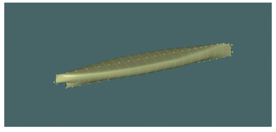Figure  1  Schematic diagram of the naked hull of the SSS test model

Download: Full-Size Img

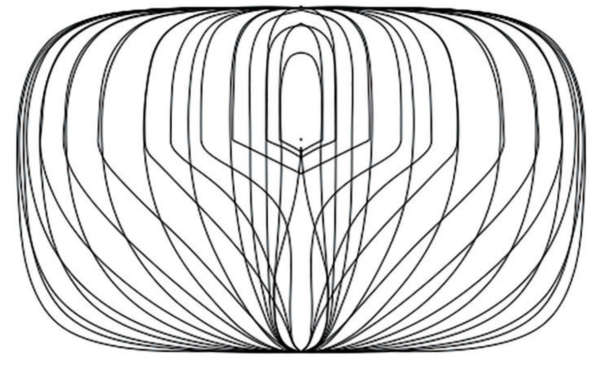Figure  2  Body line of the SSS model

Download: Full-Size Img

A bulbous bow, similar to water droplets, can be seen in the bow of the hull. The shape of the stern is similar to that of a cruiser stern in a conventional ship, and there is room for thrusters and rudders. The side top, which has an arc-shaped top side with a large radius of curvature to transition smoothly and tangentially to the deck, is the most significant difference from conventional surface ships. The overall shape is also well-integrated.

Table 1 presents the main dimensions and related overall parameters of the SSS model.

2.2   Test scheme

The scale of the ship model towing tank of the Dalian University of Technology is 160.0 m × 7.0 m × 3.7 m (length × width × water depth). Pool trailer speeds range from 0.010 m/s to 8.000 m/s with a speed accuracy of 0.1%.

Model resistance at different diving depths was tested. The resistance at 0.4 m/s, 0.6 m/s, 0.8 m/s, 1.0 m/s, 1.1 m/s, 1.2 m/s, 1.3 m/s, 1.4 m/s, 1.5 m/s, 1.6 m/s, and 1.7 m/s was tested under each diving depth. Accordingly, the range of Froude number (Fr) is 0.101 0–0.429 1, and the range of Reynolds number (Re) is 0.528 4 × 10⁶–2.245 9 × 10⁶. A total of six cases (#0–#5) were tested, and the corresponding diving depths were respectively 0 m, 0.054 m, 0.32 m, 0.48 m, 0.64 m, and 0.96 m, all based on the designed waterline. Table 2 shows the test setup, and Figure 3 depicts the resistance test site.

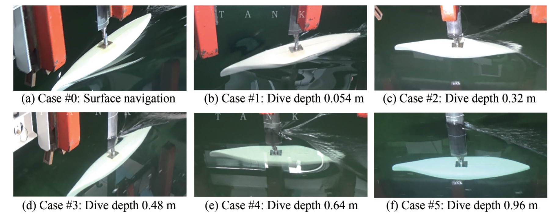Figure  3  Towing test site photos

Download: Full-Size Img

2.3   Towing test results and analysis

After each group of towing experiments, the multi-speed test results of various cases were obtained. Since the sensor is subjected to resistance due to water flow during measurement, SSS's resistance is equal to the difference between the resistance measured with the sensor and the resistance of the single sensor. Table 3 depicts the resistance of SSS by analyzing test data.

Figure 4 presents the curve of the abovementioned V_m−R_tm measurement results.

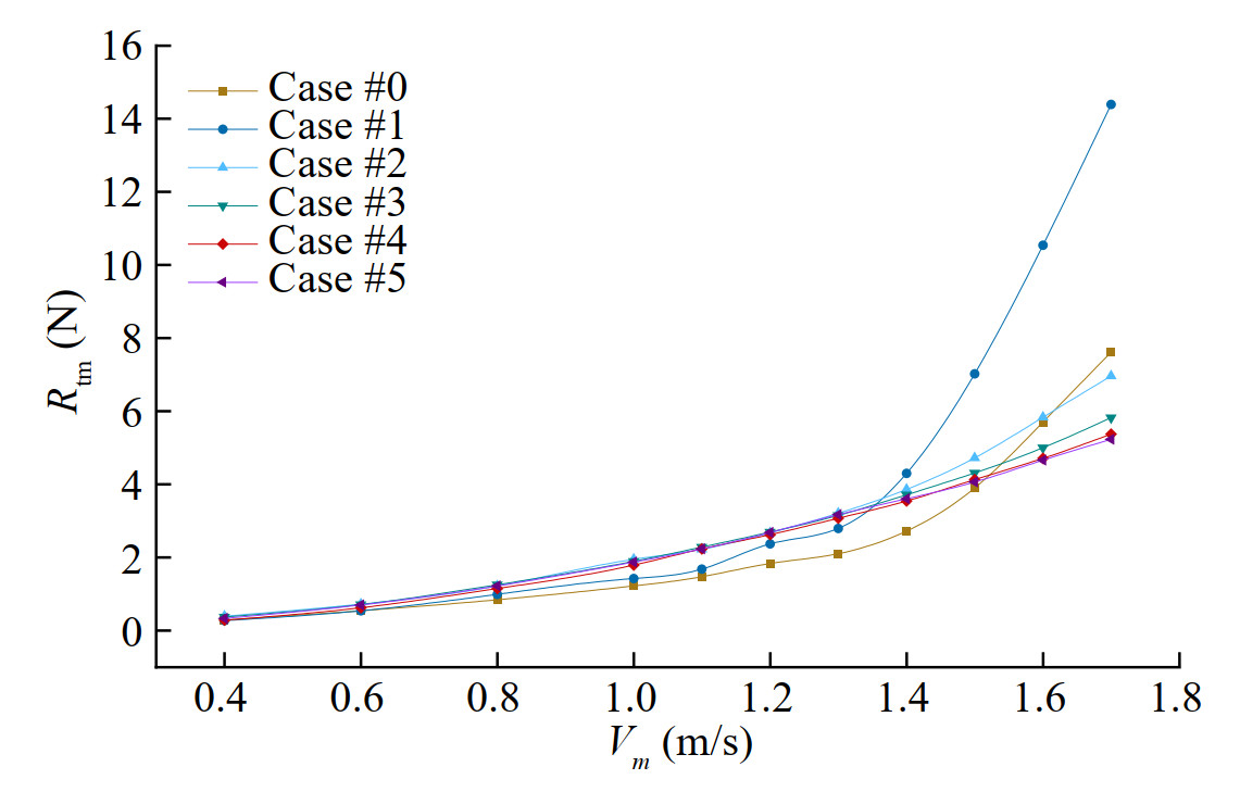Figure  4  The V_m−R_tm curve of SSS

Download: Full-Size Img

As shown in Table 2 and Figure 5, the resistance performance of SSS is analyzed as follows according to the relative position of the ship and water and speed changes in various cases:

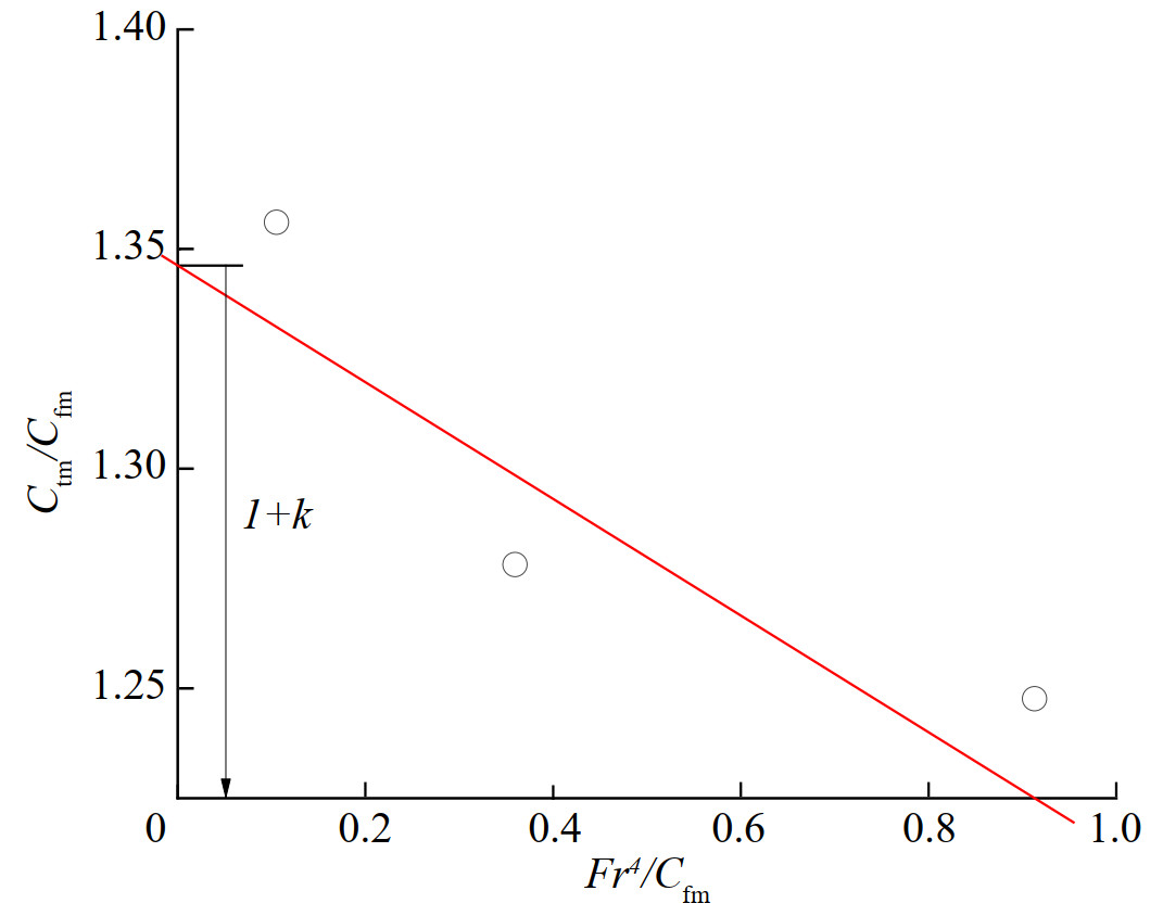Figure  5  Prohaska method to determine form factor

Download: Full-Size Img

1) When V_m is 0.4–0.8 m/s, the difference in resistance of each case is not significant. Therefore, the ship's resistance for surface navigation and submerged navigation are similar, and the trend of resistance increases with the increase in speed is not obvious. The resistance of Case #0 is slightly lower than in other cases, and the resistance of Cases #2–#5 has no obvious change in direct proportion to depth.

2) When V_m is 1.0 – 1.3 m/s, Case #0 and Case #1 (in which the upper surface of SSS coincides with the water surface) are significantly smaller than Cases #2–#5. However, the difference in resistance of each underwater case is not obvious. This shows that no violent wave-making occurs when sailing on the water surface at this speed. Most resistance components are friction resistance, which strongly correlates with wetted surface area. The particularity of Case #1 is that the upper surface of the hull and water surface theoretically coincide, but a wetted surface does not completely cover the hull due to fluctuation of the water surface during sailing. Specifically, the upper deck and surface close to the wetted surface area have no obvious wet effect, and their friction resistance is thus reduced.

3) When V_m is 1.4 – 1.7 m/s, Fr reaches 0.35 or more, which is categorized as high-speed sailing. At this time, the wave effect of SSS tends to be significant, so the resistance of Case #0 and Case #1 has an obvious positive trend with speed. Because increasing wave-making effect with increasing speed changes the resistance component of the hull, frictional resistance is gradually replaced by wave-making resistance as the main component of resistance at high speed. When speed is 1.7 m/s, due to violent wave-making and the flapping of irregular water surface on the upper surface of the hull, the increase in wave resistance with speed goes with V⁵. Simultaneously, according to the Smith effect, wave characteristics of fluid particles below the water surface decay exponentially. As a result, the resistance of various underwater cases also decreases with increased depth, and this trend becomes more significant with increased speed. The resistance difference between Case #4 and Case #5 is insignificant in this entire speed range, indicating that the influence of fluid particles by surface wave fluctuation in this diving depth range has nearly disappeared.

3   Real-scale resistance prediction method

ITTC1978 ship model test extrapolation method (threedimensional method) has been widely used worldwide. The resistance coefficient of the real-scale ship can be expressed as

where k + 1 is the form factor; C_fs is the frictional resistance coefficient; C_r is the residual resistance coefficient; ΔC_f is the roughness coefficient; C_AA is the air resistance coefficient.

For the frictional resistance estimation of the realscale ship, the Grigson formula shows higher prediction accuracy than the ITTC1957 formula, and its formula is as follows:

where L_pp is the length of the ship; V is the trailer speed; v is the kinematic viscosity coefficient.

The roughness coefficient becomes

where the roughness performance K_s = 0.15 mm.

where A_T is the projected area of the hull above the waterline on the middle cross section; S is the wet surface area.

In this study, the air resistance has little effect on the total resistance, so the effect of air resistance is ignored.

According to the test results in the range of Fr = 0.1–0.2, the form factor (1 + k) was determined.

In Eq. (5), C_tm, C_fm, and Fr can be obtained from the ship model resistance test data. The C_tm/C_fm and Fr/C_fm are plotted linearly. And the intercept of the line is then the form factor 1 + k, as shown in Figure 5. Finally, the form factor 1 + k is determined to be 1.34.

4   Numerical calculation method

This study was based on the RANS method. The SST k−ω turbulence model was used to study the SSS resistance and flow field characteristics at different scales. A VOF model was used to capture the free surface.

4.1   Calculation of objects and case

The parameters of the model scale and real-scale SSS are shown in Table 4, and the geometric model is shown in Figure 7.

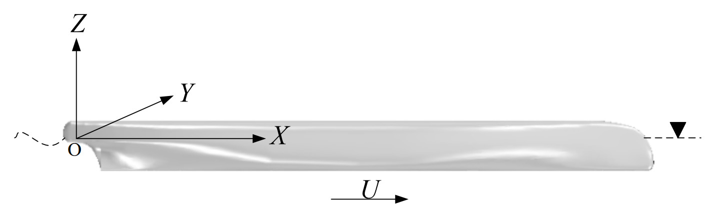Figure  6  Geometric model

Download: Full-Size Img

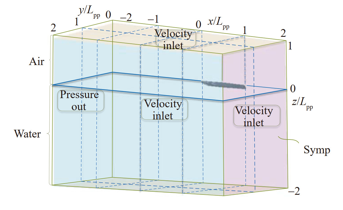Figure  7  Boundary condition display diagram

Download: Full-Size Img

4.2   Computational domain and mesh generation

During numerical simulation, SSS is in a state of uniform linear motion on the water surface. A geodetic coordinate system was used to study the problem, with X-axis pointing to the bow as positive, Y-axis pointing to the starboard side as positive, and Z-axis pointing up as positive. The issue of SSS sailing at a constant speed can be transformed into a problem of water flowing around the submarine. The hull has strict symmetry; thus, 1/2 symmetry was used to simulate the SSS model. The origin of coordinates was defined as the intersection of the vertical line of the stern and the design waterline, the distance from the bow one time the length of the SSS as an entrance, and the distance from the stern two times the length of the SSS as an exit. The hull distance to the upper boundary of the calculation domain was one time the length of the ship, and the lower boundary of the distance calculation domain was two times the length of the ship. To better present Kelvin waves in their entirety, the shipboard distance from the side boundary of the computational domain was two times the length of the ship. The cutting body of software was used to divide the mesh. The basic grid size is L_PP/50, and the number of boundary layers, boundary layer growth rate, and Y+ settings of model scale and real-scale are shown in Table 5. Mesh refinement was performed on bow and stern, free surface, calculation domain, and obvious wave-making areas to ensure accuracy of numerical simulation calculations. Figure 7 depicts the boundary conditions, whereas Figure 8 presents the meshing diagram at the real scale and model scale.

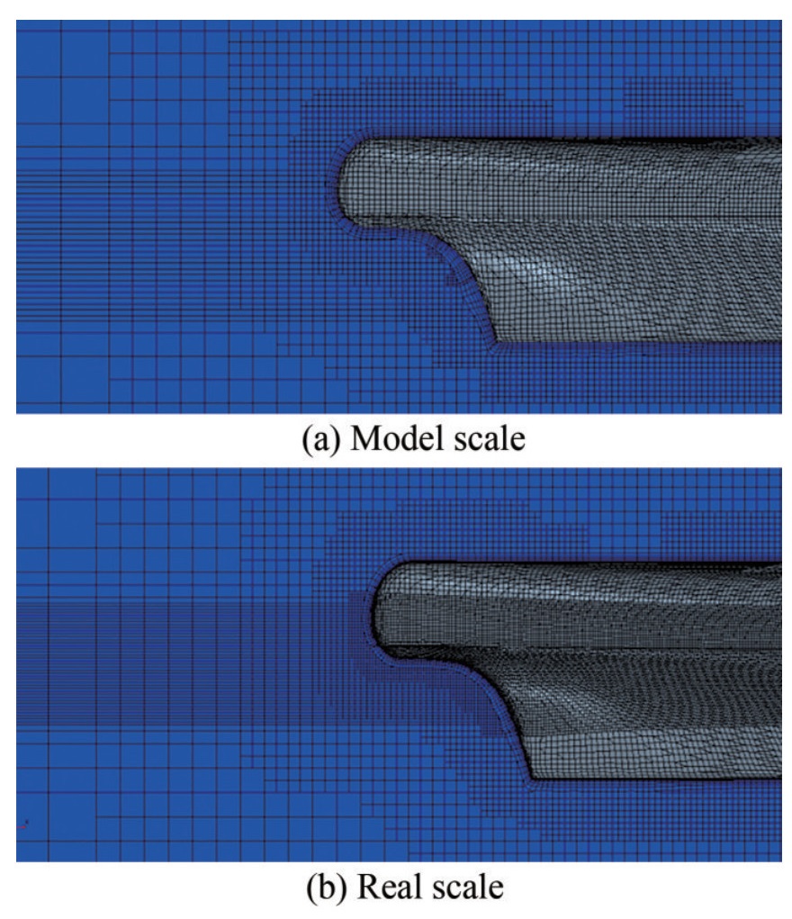Figure  8  Meshing diagram

Download: Full-Size Img

4.3   Numerical calculation result comparison

In order to confirm the correctness of the mesh topology used in this study, the mesh independence analysis was carried out on the model scale ship and the real-scale ship with Fr = 0.202. The mesh-independent validation was carried out based on the Richardson extrapolation. Three sets of meshes with different numbers were generated, the time step of the model scale was taken as 0.005 L_pp/V according to the recommendations of ITTC regulations, and the time step of real-scale calculation was taken as 0.002 5 L_pp/V.

Tables 6–8 depict the results of resistance deviation and independence analysis, where C_t is the resistance coefficient of the model scale as the test result of the SSS model; the resistance coefficient of the real-scale ship is the extrapolated resistance value based on the SSS model test; R_G is the mesh convergence rate; U_G is uncertainty; D₀ is the corresponding test (extrapolation) result; P_G is the accuracy order.

Table 8 shows that the resistance calculation results of the three sets of mesh at the model scale have high accuracy, and the deviation is within 7%. The mesh convergence rate R_G of the two scales is less than 1, indicating that the mesh converges monotonically. The numerical uncertainty U_G of model scale and real-scale resistance is 0.176%D₀ and 0.742%D₀ (less than 1%D₀), indicating a high level of numerical simulation verification. In general, this mesh topology has good convergence and can be used to study the scale effect of ship resistance. The subsequent two-scale calculations are based on the coarse mesh, and the time cost can be reduced.

5   Results and analysis

5.1   Ship resistance

The comparison of the resistance calculation results of the CFD model scale, experimental model scale, CFD real scale, and real-scale extrapolation is shown in Figure 9. It can be seen from Figure 9 that the CFD real-scale results and the extrapolation results are in good agreement, and the average difference is 5.27. It shows that the extrapolation results can be used to replace the numerical simulation results to a certain extent, and the time cost can be reduced. By comparing the results of the CFD real scale and CFD model scale, it is not difficult to find that under the same Fr, the total resistance has an obvious scale effect.

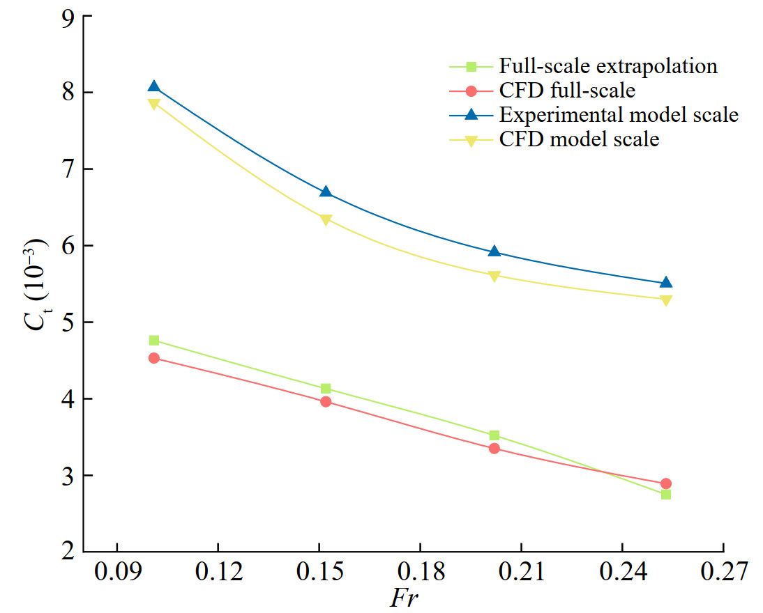Figure  9  Comparison of resistance at different scales

Download: Full-Size Img

5.2   Scale effect of the surrounding flow field

Scale effects arise due to dissimilarities in force ratios between model and real-scale ships (Terziev et al. 2020). Therefore, studying the scale effect when solving the real-scale hydrodynamic performance is necessary.

Figure 11 shows the distribution of the hydrodynamic pressure coefficient (C_P) on the hull of the model scale and real scale for Fr = 0.404.

where P is the total pressure, ρ the density of water, g the acceleration of gravity, h the water depth, and V₀ the speed.

Figure 10 shows that the hydrodynamic pressure distribution of the hull under the model scale and the real scale has a high similarity, but there are certain differences in the bow and stern. The hydrodynamic pressure of the bow at the real scale is slightly larger, reflecting that the wave-making at the bow has a specific scale effect. The pressure coefficient at the stern is smaller at the real scale, mainly due to the smaller viscous force. The difference in the distribution of pressure coefficients at the model scale and realscale explains the reason for the scale effect of the form factor.

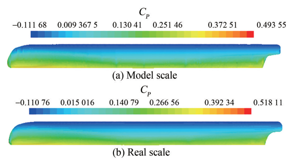Figure  10  Surface pressure distribution of ships at different scales

Download: Full-Size Img

Figure 11 shows the model scale and real-scale free surface waveforms when Fr = 0.404. Moreover, the waveform at the two scales has a high similarity, as presented in Figure 11. However, the amplitudes of the bow and stern waves at the model scale are significantly lower, resulting in a weakened prediction of the wave-making resistance at the model scale.

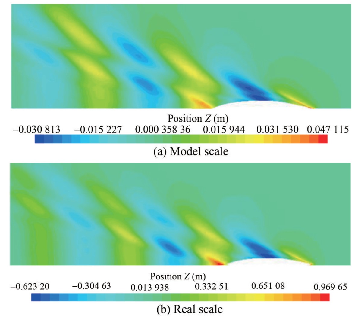Figure  11  Free surface waveforms

Download: Full-Size Img

6   Neural network prediction model

6.1   Sample data acquisition

According to the previous SSS resistance test data (Table 3), 55 sets of sample data were obtained (due to the special case of working condition 1, the data of working condition 1 were discarded). V and D^* of the SSS were used as the network input, and the sailing resistance was used as the output of the prediction network model.

6.2   K-fold cross-validation

The flowchart in Figure 12 shows that first, the data are randomly divided into K groups, and then, for each group, the following operations are performed:

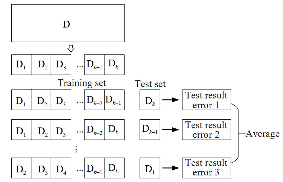Figure  12  K-fold cross-validation flow char

Download: Full-Size Img

• One training fold was chosen as the test dataset.

• The remaining K−1 is used as the training set.

• The selected training dataset is used to train the model, and the test dataset is used to evaluate it.

In the small sample dataset of this work, K was set to 5. Neural network simulation results in low bias and moderate variance results were directly utilized. Therefore, in this simulation, the comprehensive data set was randomly divided, 44 groups were selected as the training set, and the remaining 11 groups were used as the test set. The 44 sets of samples were then divided into five training folds. Furthermore, each time, a different test fold from D₁ to D₅ is chosen as the validation set. Then these five sets of data are input into the back propagation neural network (BPNN) model. The inaccuracy of model evaluation caused by accidental segmentation of the sample dataset can be ruled out with five cross-validations.

6.3   BPNN and genetic algorithm

Based on the advantages of BPNN, such as nonlinear mapping ability, self-learning adaptive ability, generalization ability, and fault tolerance ability, the applicability of BPNN in predicting the SSS resistance is discussed.

The activity level of neuron j in layer L is:

The tansig activation function is:

Neural network weights:

In the formula, the "δ" of the output layer and the hidden layer are respectively:

The empirical value of "α" is selected between 0 and 1, and the learning rate η=0.01.

In the BPNN, the neural network has a nonlinear mapping ability and is suitable for solving problems with complex mechanisms, so the neural network can predict the output of nonlinear functions. It can get random weights and thresholds from the split samples and start training the model. Regarding the genetic algorithm (GA) part, the steps of calculating fitness value, crossover, mutation, etc., select the optimal group until it is close to the optimal solution (Ferreira 2001). In general, GA adopts binary coding and divides the program into four parts: input and hidden layer link weights, hidden layer weights, hidden layer and output layer weights, and output layer weights. Each weight and threshold is coded with m-bit binary, and then the optimized weight and threshold are input to the BPNN.

6.4   Model parameter settings

In this study, 55 sets of data were selected as training and testing samples for development. The sum of the absolute values of the prediction errors of the training data is used as the fitness value of the individual. The smaller the fitness value of the individual is, the better the individual is.

To achieve the optimal simulation of the BPNN model, the number of neurons in the hidden layer needs to be changed according to the learning rate, number of neurons, learning algorithm, etc., and is determined after many experiments (Nguyeo 2019). In addition, it is assumed that the number of hidden layer neurons is 2−12. In addition, the simulation results of BPNN are used to test the optimal number of neurons (the predicted results are shown in Figure 13). The main purpose of this study is to improve the predictive model through a K-fold cross-validation approach. During this process, when the number of neurons in the hidden layer changes, it is difficult to determine whether the prediction results are changed by the K-fold cross-validation method. Therefore, controlling the number of neurons in the hidden layer can provide a more intuitive view for this method. Figure 14 shows the final network structure of the neural network used in this study for SSS resistance prediction.

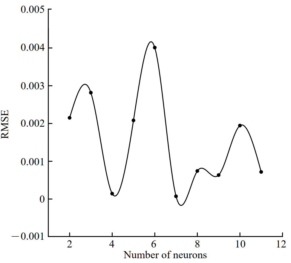Figure  13  Average test error of 5-fold cross-validation for different neuron models

Download: Full-Size Img

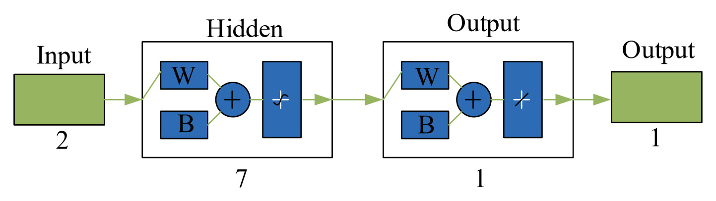Figure  14  Neural network structure

Download: Full-Size Img

In the BPNN, the number of samples was randomly divided into two groups, the first group of 44 samples was used for training, and the remaining 11 samples were used as test samples. This can better illustrate the authenticity of the simulation results. In the GA-BPNN, the number of samples is also divided, but the weights and thresholds vary with the best gene individuals selected. The GA parameters were set as follows: the total population size of the genetic algorithm was 20, the maximum number of iterations was 30, the crossover rate was 0.8, and the mutation probability was 0.1.

6.5   Evaluation indicators

This paper used five statistical evaluation indicators to evaluate the performance of different models. They are mean absolute error (MAE), mean square error (MSE), root mean square error (RMSE), coefficient of determination (R²), and mean absolute percentage error (MAPE).

These metrics are calculated as follows:

In Eqs. (12)−(16), n is the number of data sets, y is the average value of the test resistance of the SSS, ${\hat y}$ is the predicted resistance value, and y_i is the test resistance.

MSE, MAE, and RMSE are measures of mean error and are used to assess the degree of variability in the data. Also, RMSE has a smooth loss function. Furthermore, R² is used to characterize the fit by the variation of the data. Its normal range is [0, 1], and the closer it is to 1, the better the variable y in the equation explains, and the better the model fits the data. Additionally, MAPE can determine how well different models evaluate the same data; the lower the value, the better the prediction.

6.6   Model prediction performance comparison

The K-fold cross-validation method is used to sequentially select training samples as input data, and then BP and GA-BP neural networks are used to predict the resistance of the SSS. Table 9 shows the results, which presents the K-fold cross-validation results for five different datasets. This step selects the model with the best predictive performance by comparing the evaluation metrics. Although some test groups had high correlation values close to 1, they performed poorly on the RMSE and MSE measures.

After K-fold cross-validation, Table 9 shows that the best model should be group 5, and the MAE, MSE, and RMSE values in group 5 are lower than in other models. In Table 9, evaluation metrics can be used to evaluate the predictive performance of each group of models. The smaller values of MAE, RMSE, and MAPE improve the generalization ability of the prediction model. Also, R² is informative, and the value of a perfect model should be closer to 1. Therefore, when the MAE exceeds 0.1, groups 2, 3, and 4 should be discarded. Moreover, the R² evaluation metric also provided a reason to exclude the first group because the R² value corresponding to group 1 (0.994) was smaller than that of group 5 (0.998). Therefore, group 5 was selected comprehensively. Then, the weights and thresholds were recorded and fed into the BPNN model for comparison with the test set. After the initial weights and thresholds were changed, the prediction model of the BPNN was also improved.

Figure 15 shows that GA and K-fold cross-validation work well to improve the prediction accuracy of BPNN, including the error ranges for different models. Figure 4 depicts that the maximum error of the neural network model using K-fold is reduced from 0.25 to 0.1. Similarly, the maximum error of the GA-BPNN model is reduced from 0.25 to 0.07. Furthermore, most of the 11 test data errors of GA-BPNN are closer to 0 (Figure 15), showing that for this study, GA is better than K-fold cross-validation in reducing error.

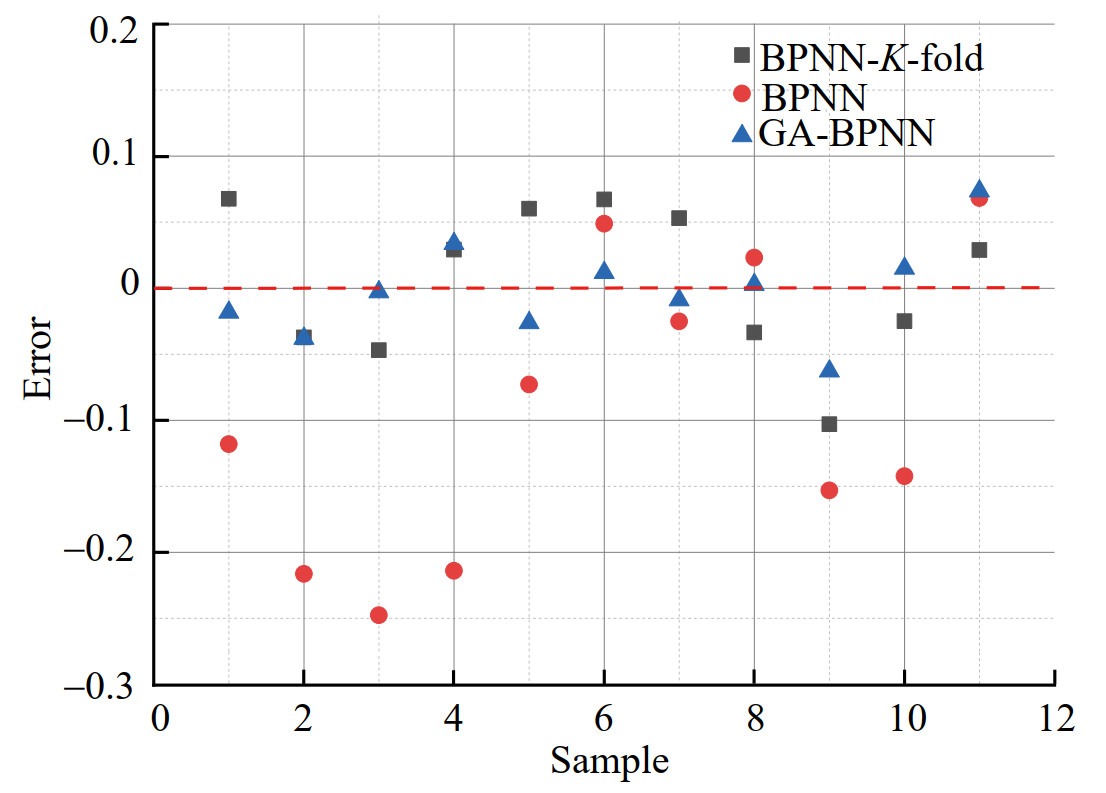Figure  15  Error distribution between different models

Download: Full-Size Img

The predicted value of the BPNN model has a higher error value than that of the GA-BPNN. In particular, the prediction errors of groups 1–5 of the BPNN are larger. This result is because fewer data are selected for training, and the threshold and weight derivation of BPNN are limited. After optimizing the thresholds and weights by GA, the BPNN also performed well (Figure 16). And both models achieved good results in the last five test data. However, the 5th group error of the neural network model using K-fold is too large (as shown in Figure 18). Overall, the prediction results of the GA-BPNN are in good agreement with the actual values.

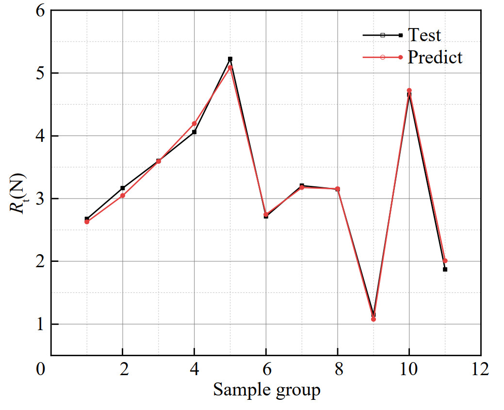Figure  16  Prediction results of GA-BPNN

Download: Full-Size Img

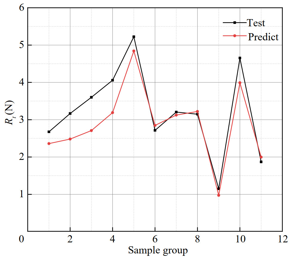Figure  17  Prediction results of BPNN

Download: Full-Size Img

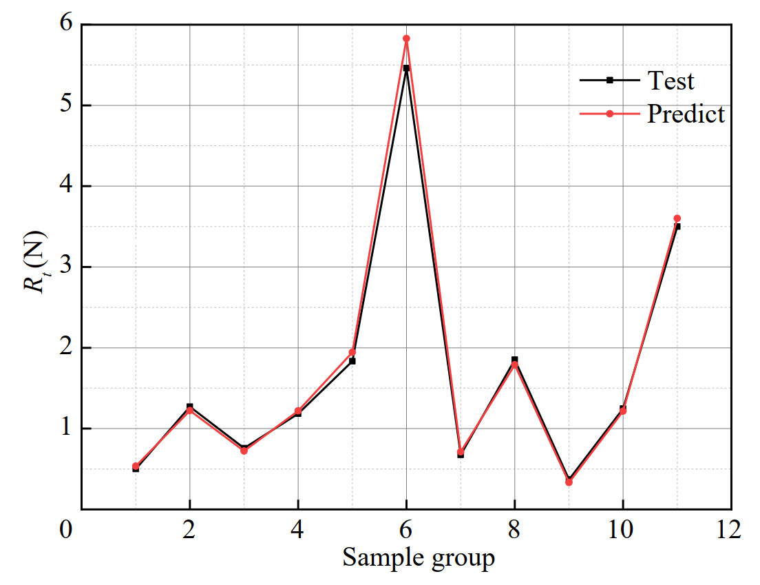Figure  18  BP neural network optimized by K-fold cross-validation

Download: Full-Size Img

BPNN generally performs poorly without parameter optimization due to the random generation of thresholds and weights. A GA can find the optimal weights and thresholds. Also, by entering the weights and thresholds filtered by K-fold cross-validation, the network can be improved.

The reciprocal of MAE, MSE, RMSE, MAPE, and R² are plotted as a radar chart of model performance evaluation metrics, as shown in Figure 19. Through K-fold cross-validation optimization, the fit of the model is improved, R² is improved from 0.895 to 0.998, but the MAPE is only reduced by about 0.07. Furthermore, BPNN optimized by GA has a better effect than BPNN. The values of MAE, MSE, RMSE, and MAPE all decreased, and the correlation coefficient increased by 0.1. This result is better than the neural network after K-fold cross-validation. Compared with the neural network after K-fold cross-validation, the GA significantly impacts the optimization of the neural network by setting better initial weights and thresholds. The simulation results show that although K-fold cross-validation also has a specific optimization effect on the neural network, the improvement is insufficient. However, after optimization by GA, the RMSE, MSE, MAE, and MAPE values of the neural network model are the lowest (as shown in Table 10), and the optimization effect is the best.

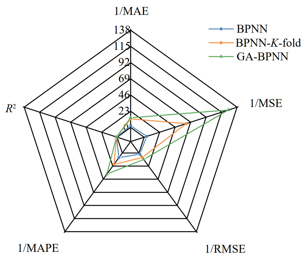Figure  19  Model performance evaluation index radar chart

Download: Full-Size Img

7   Conclusions

This study aims to investigate the performance of the optimized BPNN in predicting the resistance of SSS. By entering different V and D, the resistance performance of the SSS in multiple sailing states is studied. The specific conclusions are as follows:

1) By analyzing the results of the resistance test and numerical simulation, it can be found that when an SSS is sailing at medium or low speed (V_m = 0.4–1.3 m/s), the effect of different cases on the resistance performance is not obvious. At high speeds (V_m = 1.4–1.7 m/s), the resistance of the edge diving case (Case #1; that is, the upper surface of the ship coincides with the water surface) and the surface case (Case #0) increases sharply with the increase in speed.

2) In this study, the resistance performance of SSS in various scales is solved based on the RANS method. The hydrodynamic pressure of the bow at the real scale is slightly larger, reflecting that the wave-making at the bow has a specific scale effect. The wave amplitudes of the bow wave system and the stern wave system at the model scale are significantly lower, resulting in a weakened prediction of the wave-making resistance at the model scale.

3) In this paper, the original data are normalized to ensure that the dataset is easier to use. The 55 sets of experimental data come from the resistance test results done by the author. The dataset is randomly divided into two groups: the first group contains 44 sample data for model training and validation; the remaining data are used to verify the accuracy of the model. In this paper, BPNN is used, and GA and K-fold cross-validation are used to optimize the network parameters of the model. After K-fold cross-validation models, the five groups of data, in turn, optimize the initial threshold and weight of BPNN. Conversely, the genetic algorithm finds the optimal thresholds and weights in successive iterations. However, both methods improve the accuracy of BPNN prediction results. But based on the statistical results of MAE, MSE, RMSE, MAPE, and R², GA-BPNN is the best predictive model for SSS resistance.

4) As a new type of ship, research on the fast performance of the SSS has potential application value in the engineering field. In the next step, we can combine the innovative design of ship form and introduce complex marine environment elements such as waves and ice loads for more in-depth research.

Nomenclature