1   Introduction

Supercavitating projectiles are weapons launched by artilleries, and fly with very small drag by using supercavitation drag reduction technology. Supercavitating projectiles fly underwater by consuming initial kinetic energy, and destroy small underwater objectives by the hit-to-kill mode, so is not equipped with any explosive and propulsion devices (Saranjam, 2013). A well-designed projectile can fly 100 m underwater, the residual speed is still higher than 200 m/s, and the residual kinetic energy is strong enough to break down a 100 mm-thick steel plate (Zhao et al., 2021). To achieve a larger defensive range and stronger lethality, a higher initial speed of supercavitating projectiles is expected. Currently, launching speed of small-caliber artilleries can be up to 1 800 m/s, and can be further increased to 3 000 m/s if electromagnetic guns are used (Yao et al., 2017). Therefore, it is necessary and realizable for supercavitating projectiles to achieve the underwater supersonic speed, which is higher than 1 483 m/s.

However, supercavitating projectiles encounter new challenges when flying with a high-speed approaching the sonic speed in water (Yao et al., 2017; Wang et al., 2020). For example, when the speed is approximately equal to 1 500 m/s, the stagnation pressure ahead of cavitator can be up to 1.1 GPa. Given that the bulk modulus of water at room temperature (about 25 ℃) is only 2.2 GPa, so the water compressibility can't be ignored (Serebryakov, 2003). Further, a bow shock occurs when supercavitating projectiles flies in supersonic conditions, which exerts significant influences on the flow regime, supercavity shape, and hydrodynamic characteristics (Al've, 1983). Resultantly, the flow field characteristics are totally different from that of conventional supercavitating vehicles (~100 m/s).

A series of experimental and numerical investigations on high-speed supercavitating projectiles were previously carried out. In 1983, Al've numerical studied the subsonic, transonic and supersonic flow field of water around a cone at the first time, and pointed out that the drag coefficient is not a constant and depends on the Mach number (Ma) (Al've, 1983). Savchenko et al. carried out experiments of subsonic supercavitating projectiles, obtained the supercavity in high-speed condition, and believed that the stagnation pressure coefficient before the cavitator increases with speed because of water compressibility (Savchenko et al., 1993). Jenkins et al. experimentally investigated the external flow field of a supersonic supercavitating projectile and an underwater bow shock is observed by using a high-speed camera (Jenkins and Evans, 2004). Hrubes et al. investigated the supercavity shape and motion stability of the high subsonic (Ma 0.654) projectile and supersonic (Ma 1.032) projectile by high-speed photography, and also studied the formation mechanism of the underwater bow shock (Hrubes, 2001). Savchenko et al. pointed out that the underwater bow shock strongly influences the supercavity shape (Savchenko, 2001). Dyment et al. studied the relationship between the water compressi-bility and flow speed by studying the impingement of a high-speed flow on the stationary rigid body, and obtained the influence of a high-speed rigid body on the free surface of water (Dyment, 2015).

To predict the supercavity shape and the hydrodynamic characteristics of cavitator, the subsonic, transonic, and supersonic flow fields underwater are also analytically solved. Serebryakov built a method to predict the supercavity behind a slender cavitator in subsonic and supersonic flow field by using the matched asymptotic expansion method (MAEM) (Serebryakov, 1992). MAEM was also adopted by Wang et al. to calculate the supercavity produced by slender cones in high-speed supercavitation flow (Wang et al., 2017). However, MAEM is suitable for slender cavitators, of which the angle between the tangent lines of cavitators and supercavities at the initial point of supercavity should be no more than 10°, and the calculation precision decreases as the angle increases. For disk cavitators and blunt cone cavitators, MAME can't calculate the supercavity accurately (Serebryakov, 1994). In addition, Serebryakov (Serebryakov, 1994) also held the idea that the results calculated by the developed asymptotic theory is uncertain for the transonic region, and it is hard to build a unified correlation to describe the supercavitation flow regime in the subsonic, transonic, and supersonic region. Li et al. theoretically analyzed the influence of projectile speed on the position and shape of underwater bow shock and the flow parameters ahead and behind the bow shock (Li et al., 2018). Further research shows that the supercavity produced in high-speed condition significantly influenced by Ma, and the influence laws for blunt cavitators are very different from that for slender cavitators (Serebryakov, 2001).

According to the published literature, water compressibility has significant influence of the flow regime, supercavity shape, and hydrodynamic characteristics for high-speed supercavitating projectiles, and must be considered. Although the experiments of high-speed projectile have been conducted, the effective results are insufficient because of limited testing method in so high-speed underwater conditions, particularly for supersonic projectiles. Numerical simulations are focusing on the computational method for compressible supercavitation flows and the capturing method for underwater shocks. Analytical method has a poor accuracy for solving the transonic and supersonic problems in water. In addition, most of the published results focus on the slender cavitator. The flow regime of high-speed water pasting a slender cavitator is obvious different from that of a blunt cavitator. Although blunt cavitators, especially disk cavitators, are mainly used as the cavitator of supercavitating projectiles because of the good stability of motion (Mansour et al., 2020), the relevant results are rare. The influences of water compressibility and underwater shock on supercavity shape and hydrodynamic characteristics are not explained quantitatively and the mechanism is also unclear. These problems are essential to further explore motion characteristics of high-speed supercavitating projectiles.

In this paper, the compressible supercavitation flow field of supersonic supercavitating projectiles during the deceleration process (from supersonic speed to subsonic speed) is studied using the computation fluid dynamic (CFD) method. The quantitative influence of the speed on the supercavity shape and hydrodynamic characteristics in the range of 200–1 800 m/s are explained. The remainder of this paper is organized as follows. The numerical model applied to the compressible supercavitation flow field is first established, followed by the model validation. Then, the supercavitation flow regimes around a supercavitating projectile with a disk cavitator in the compressible and incompressible waters at different speeds are numerically calculated and compared. The influences of water compressibility and flying speed on the supercavity shape and hydrodynamic characteristics of supercavitating projectiles are finally obtained.

2   Numerical model

2.1   Governing equations

The external flow field of supercavitating projectiles includes a two-phase flow and a mass transfer between vapor and water, and a clear and stable interface exists between the two phases. Volume of fluid (VOF) model is an effective method to solve multiphase flow fields, and especially suitable for the flow filed of which the interactions between different phase is not very strong and the interface is continuous and stable (Wang et al., 2017; Li et al., 2018). The VOF model solves only one set of momentum equations and calculates multiphase flow by tracking the volume fraction of each phase, and is featured by high computational efficiency and strong adaptability for dealing with complex flow problem. Since the temperature increase is not significant, the energy equation is neglected when modeling the flow field of supercavitating projectiles. The basic control equations consist of the mass conservation equation and the momentum conservation equation. In addition, the gravitational force is not taken into account because of the large Froude number (Xu et al., 2021).

For the q^th phase of multiphase flow, the mass conservation equation is written as follows.

where, α_q is the volume fraction of the q^th phase; v denotes the velocity, m/s; ρ_q is the density of the q^th phase, kg/m³; ${{\dot m}_{pq}}$ and ${{\dot m}_{qp}}$ represent the mass transfer rate between the p^th phase and the q^th phase, kg/(m³·s); n is the total number of all the phases, and n=2 for the supercavitation flow field.

To close the mass conservation equation, a relationship describing the sum of the volume fraction of each phase is supplemented as follows.

In a control volume, the momentum conservation equation based on the average density and the average kinetic viscosity can be described as follows.

where, ρ_m is the average density of all the phases, kg/m³; μ_m is the average kinetic viscosity of all the phases, N·s/m². ρ_m and μ_m can be expressed as follows.

The mass transfer rate between water and vapor in the mass conservation equation can be calculated by a cavitation model. Schnerr-Sauer cavitation model has the advantages of simple form, high computational efficiency, and strong numerical stability (Huang et al., 2015), which is expressed as follows.

where, $\dot{m}_{e}$ is the evaporation rate, kg/(m³·s); $\dot{m}_{c}$ is the condensation rate, kg/(m³·s); P_v is the saturated vapor pressure at room temperature, Pa; P is the local static pressure, Pa; ρ_v, ρ_l and ρ_m are the density of vapor phase, water phase and mixture phase, respectively, kg/m³; α denotes the volume fraction of the vapor phase, which is related to the quantity of microbubbles in per unit volume of water phase and the size of the micro-bubbles.

To close the control equations, a turbulence equation is included. The realizable k-ε turbulence model can achieve high simulation accuracy and strong numerical stability when used to calculating the supercavitation flow field, which is adopted in this paper (Muhammad, 2014). However, the realizable k- ε turbulence model is applicable to the fully developed turbulent flow field under the high Reynolds number conditions. Thus, a wall function is also required to accurately calculate the wall shear stress and heat flux. The scaled wall function is chosen as the supplement of the realizable k-ε turbulence model.

According to the test data, Lyons proposed an empirical correlation based on Tait equation to govern the relationship among density, pressure and temperature, and also called an improved version of the Tait equation (Lyons, 1996). This correlation is a widely accepted state equations to describe the liquid density with the changes of pressure and temperature. The effect of temperature is excluded in this paper, and the temperature is taken as a constant value of 25 ℃. Then, the state equations are simplified as follows.

where, p is the static pressure, n is the compressible coefficient of water, and takes value of 7.15, ρ and K are the density and bulk modulus of water, respectively, a and b are the constants.

The sonic speed is the propagation speed of pressure disturbance in the medium, and can be calculated as:

In the normal condition, the operating pressure is 101, 325 Pa, which is equal to the static pressure at 1 m depth underwater, the density of water is 1 000 kg/m³, and the bulk modulus of water takes value of 2.2 GPa. Substituting these parameters into Eqs. (7) and (8), the values of the parameters a and b can be calculated, a is 307.59 MPa, b is 1.09×10⁻¹³. Moreover, the underwater sonic speed at the normal condition can be calculated by Eq. (9), and the value is approximately equal to 1 483 m/s.

2.2   Geometric model

The supercavitating projectile is a revolution solid, and typically consists of two cone sections and one cylindric section. The configuration and geometric parameters of the supercavitating projectile are displayed in Figure 1. The diameter of the disk cavitator (D_n) is equal to 2.5 mm and the geometry of the projectile can be determined as shown in Figure 1.

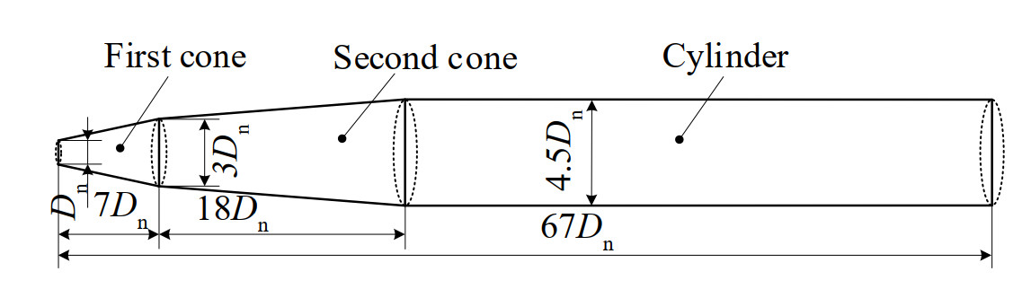Figure  1  Configuration and geometric parameters of supercavitating projectile

Download: Full-Size Img

2.3   Computation domain

The moving frame method is utilized to model the motion of supercavitating projectiles. The supercavitating projectile is regarded as a moving body, and the far field is considered as stationary. The computational domain is designed to be a large cylinder, and shown in Figure 2. The reference coordinate system is fixed with the projectile and the moving speed is equal to the flying speed of the supercavitating projectile. The pressure inlet and pressure outlet boundary conditions are utilized for the inlet and outlet, respectively. The operating depth is set as 1 m, and the total pressure at the inlet and the static pressure at the outlet are both set as 111, 125 Pa. The outer cylindrical surface is modelled as a slipping wall.

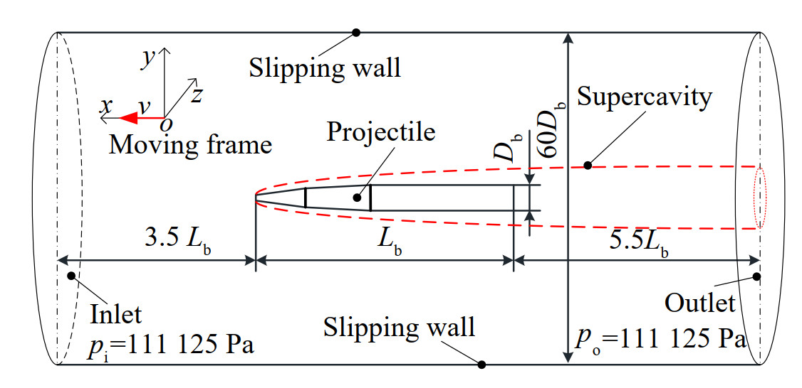Figure  2  Computational domain and boundary conditions

Download: Full-Size Img

Huang et al. demonstrates that a large enough radial extent of the computational domain is necessary to minish the influence of the boundary on the flow regime and supercavity shape, and obtains requirement of the dimensions the computational domain (Huang et al., 2015). As shown in Figure 2, the diameter of the computational domain is 60 D_b and the total length is 10 L_b, which can ensure independent calculation results. Where, D_b and L_b are the maximum diameter and length of the supercavitating projectile. The inlet is 3.5 L_b ahead of the cavitator. Since only the supercavity around the projectile is of interest, the supercavity far behind the projectile is not modelled in this paper.

Hexahedral grids are used to mesh the computational domain. The grids near walls are refined to ensure the y-plus within the range of 30 – 300 to satisfy the requirement of the turbulence model (Muhammad, 2014). The grids at the wake region and phase change region are also refined to achieve an independent result of supercavity profile. The resulting total grid number is approximately 1.2 million. Though not shown here, the grid independence study is performed.

3   Model validation

Hrubes conducted an experimental investigation of subsonic and supersonic projectiles, and the operating depth is 4 m underwater (Hrubes, 2001). The supercavity profile at the speed of 970 m/s (Ma 0.654) and the underwater shock of the case with speed of 1 530 m/s (Ma 1.032) are observed. The experimental results are used to validate the rationality of the numerical method. The supercavity profiles at the speed of 970 m/s (Ma 0.654) from numerical simulations and experimental results are compared in Figure 3. The axial and radial size of the supercavity and supercavitating projectile are normalized by the cavitator diameter (d_n =1.41 mm). Numerical simulations are performed with compressible and incompressible water to highlight the influence of water compressibility. It is shown that numerical results in compressible and incompressible water are both slightly larger than experimental results, and the relative differences are less than 5%. The comparison demonstrates the feasibility of the numerical method in simulating the subsonic supercavitation flow field. Moreover, the supercavity profile obtained from numerical simulation in compressible water is smaller and closer to the experimental results. It shows that the water compressibility slightly decreases the size of the part of supercavity near the supercavitating projectile.

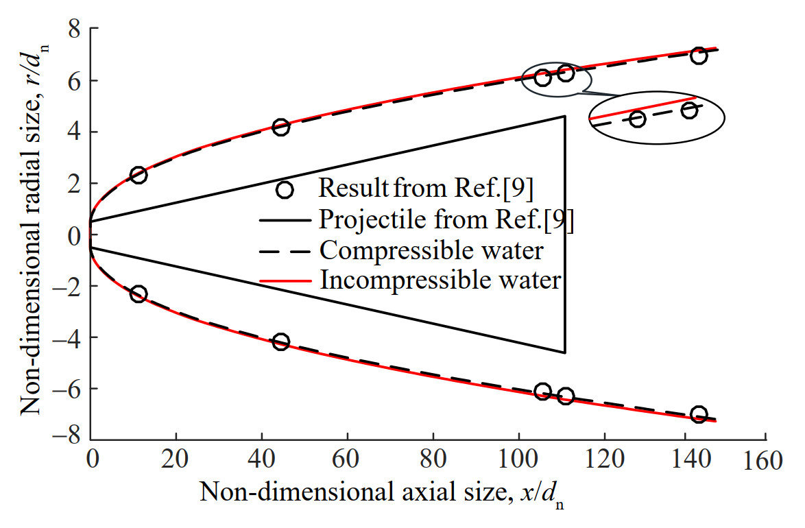Figure  3  Comparison of numerical and experimental supercavity profiles

Download: Full-Size Img

The schlieren of the underwater shock at the speed of 1 530 m/s (Ma 1.032) is also provided (Hrubes, 2001). The velocity contour in log-scale shows a bow shock in front of the projectile, which is shown in Figure 4. Therefore, the feasibility of numerical method in predicting the underwater supersonic flow filed is well validated. In addition, this case is simulated by using compressible water as fluid medium, and no underwater shock is observed by using incompressible water.

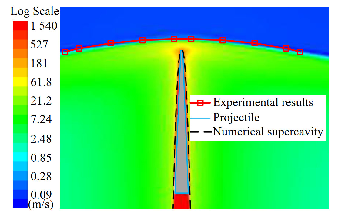Figure  4  Comparison of numerical and experimental underwater bow shocks

Download: Full-Size Img

4   Results and discussions

The initial speed of the supercavitation projectile is approximately 1 800 m/s (Ma 1.214). To produce the big enough supercavity, the ending speed must be no less than 200 m/s (Ma 0.135), which also ensures enough kinetic energy to kill targets. Therefore, the flow fields around the supercavitating projectile with the speed of 200 – 1 800 m/s (Ma 0.135 – 1.214) are simulated, and the interval value is 100 m/s. In addition, numerical simulations with incompressible water are also included as reference to highlight the influence of water compressibility.

4.1   Flow regime

The pressure contours at different Mach number (Ma 0.135–1.214) are first extracted and compared. Three representative cases, Ma 0.405 (subsonic speed), Ma 0.809 (high subsonic speed) and Ma 1.214 (supersonic speed) are chosen and displayed in Figure 5 (incompressible water) and Figure 6 (compressible water). When the water compressibility is not taken into account, the stagnation pressure ahead of the cavitator increases with Ma by square relationship, and the pressure distribution laws around the cavitator are approximately the same. However, the pressure distribution laws for cases with different Ma are totally different in compressible water, and shown in Figure 6. With the increase of Ma, the high-pressure area extends in radial direction, and shrinks in axial direction. Further, the pressure distribution exhibits the underwater bow shock for the supersonic condition.

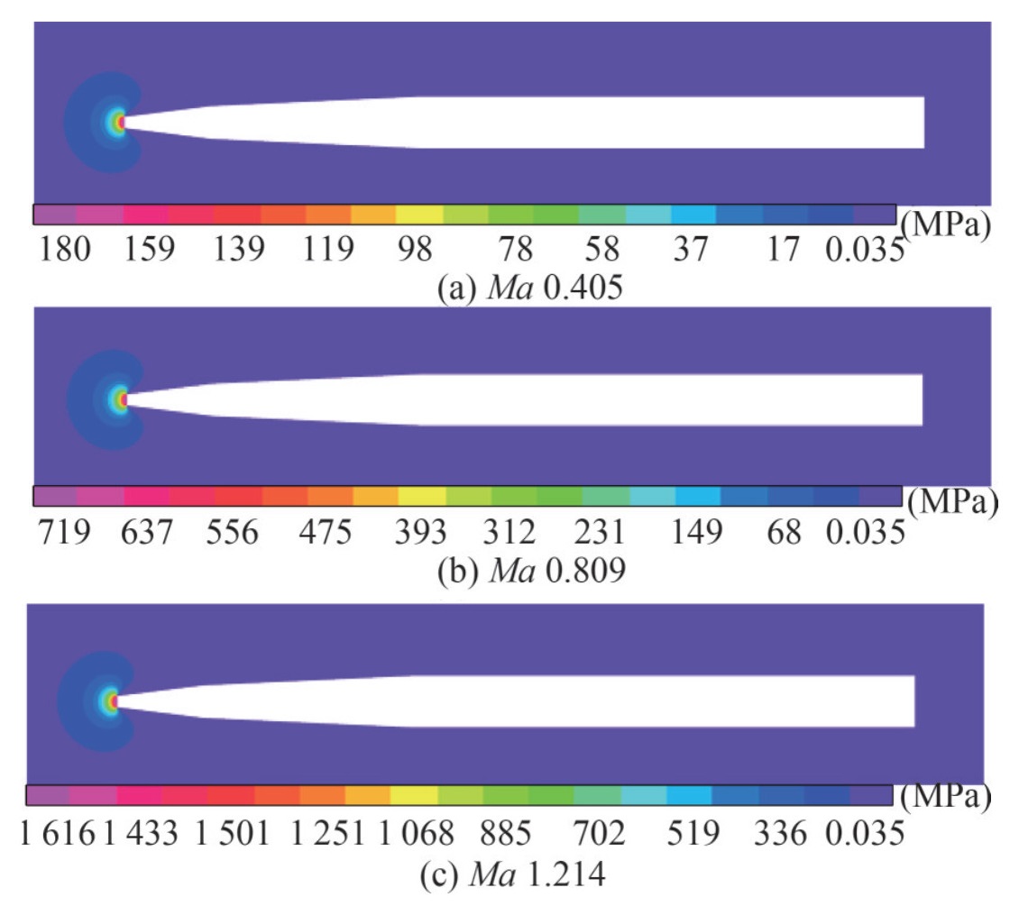Figure  5  Influence of Ma on pressure profiles when ignoring water compressibility

Download: Full-Size Img

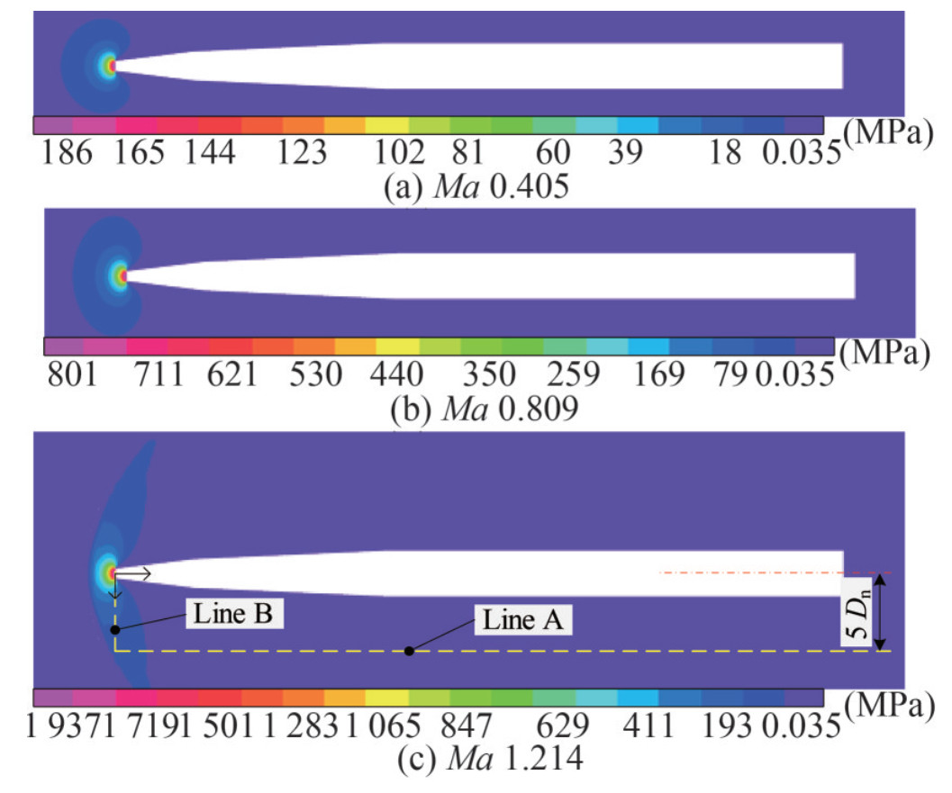Figure  6  Influence of Ma on pressure profiles when considering water compressibility

Download: Full-Size Img

By comparing the stagnation pressures of Figures 5 and 6 for the conditions with same speed, it is found that the stagnation pressure before the disk cavitator is significantly higher when the water compressibility is considered, and the difference increases with the speed. To explain this phenomenon, the relationship between static pressure and speed in compressible water is derived. The differential form of Bernoulli's equation is:

where, v is the speed of free stream, Φ is the potential function and can be regard as to zero.

Substituting Eq. (7) into Eq. (10), The following relation can be obtained.

Therefore, the compressible Bernoulli equation shown in Eq. (11) can be rewritten as:

Combining Eq. (7), Eq. (12) has the form as follows:

Eq. (13) describes the conversion relationship between the static pressure and dynamic pressure in compressible water.

The static pressure and speed of the freestream are p_∞ and v_∞, respectively, and the stagnation pressure is assumed to be p_s. Then, the conservation relationship between the freestream and stagnation point can be described as follows.

Eq. (14) can be further rewritten as:

Eq. (15) is a theoretical expression of the stagnation pressure in compressible water. For incompressible water, the stagnation pressure is equal to the sum of static pressure and dynamic pressure of far field, and can be expressed by incompressible Bernoulli equation. The change of stagnation pressure with the projectile speed in the compressible and incompressible water is displayed in Figure 7.

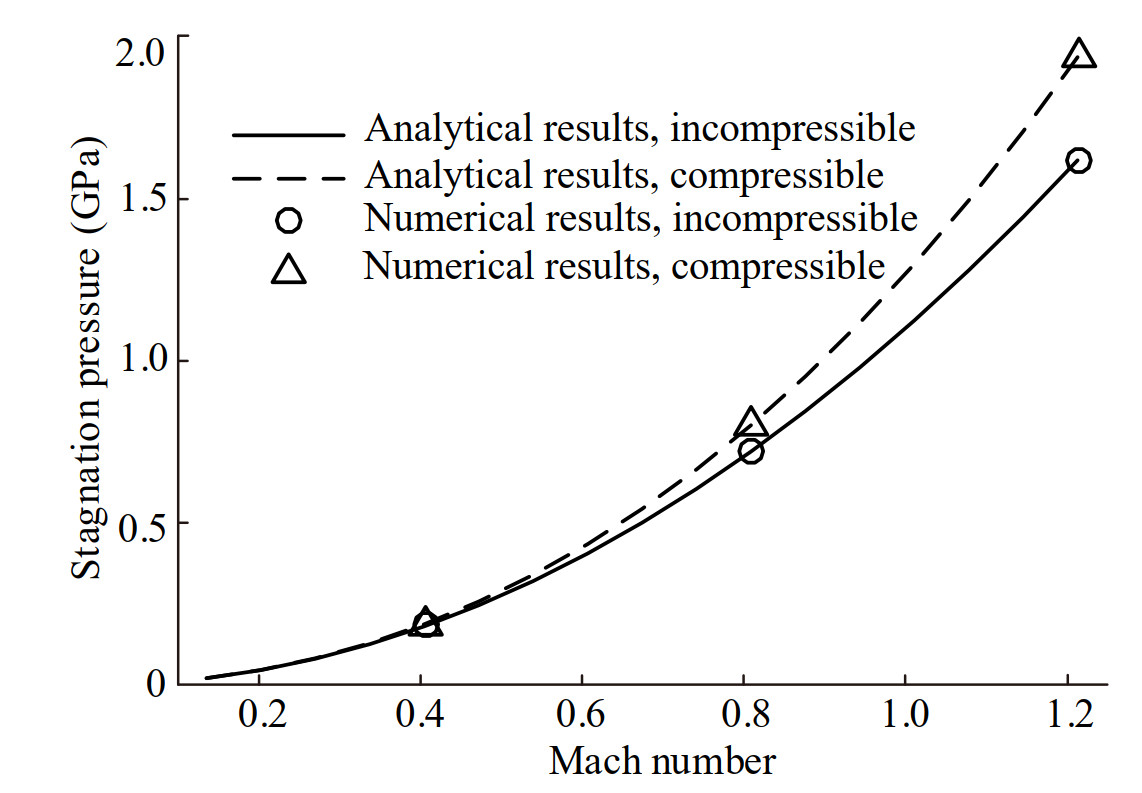Figure  7  Comparison of stagnation pressures in compressible and incompressible water

Download: Full-Size Img

It is shown that the analytical results (Eq.15) are consistent with the numerical results. The conversion relationship between the static pressure and dynamic pressure of compressible water is different from that of incompressible water. The stagnation pressure in compressible water is larger than that in incompressible water, and the difference increases with Ma.

The local pressure profile at line A (seen in Figure 6) is extracted and displayed in Figure 8. For the incompressible water, the static pressure at line A increases with Ma, and decreases gradually in the streamwise direction. By considering the water compressibility, the obtained static pressure is similar to that of incompressible water for the conditions of Ma 0.405 and 0.809. However, for the supersonic case, the static pressure sharply increases to a very high peak, and then decreases gradually because of the underwater bow shock. Further comparisons show that the water compressibility slightly increases the static pressure at the position close to the tail of the supercavitating projectile.

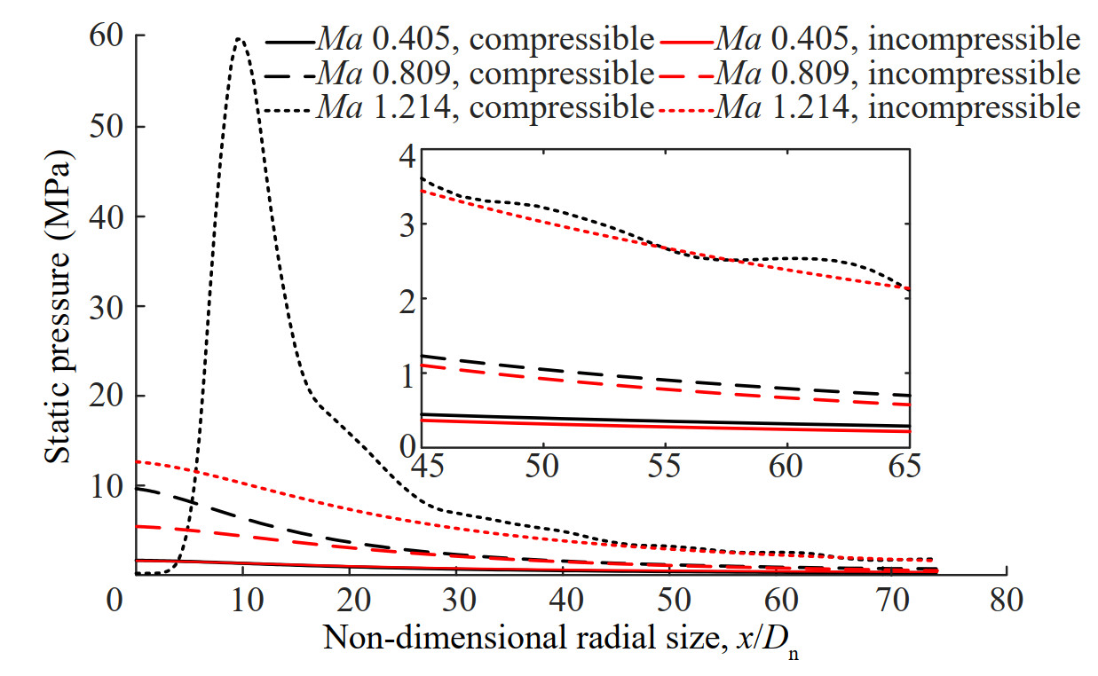Figure  8  Comparison of pressure profiles at different Ma

Download: Full-Size Img

When a supercavitating projectile flying underwater, the cavitator receives a drag and pushes the surrounding water aside. An additional radial speed is thereby produced in the water near the cavitator. The radial speed at line A is depicted in Figure 9. When the water compressibility is considered, the radial velocity at line A is approximately the coincident with the incompressible result in subsonic condition, and a gradually significant difference is found between the transonic and supersonic cases. For the supersonic condition, the radial speed increases rapidly, and then decrease gradually. The change law along the streamwise direction is obviously different from the subsonic conditions because of the underwater bow shock. In addition, For the region of line A with axial-position responding to the cylinder section of the supercavitating projectile, the radial speed in compressible water is about half of that in incompressible water in the condition of Ma 1.214.

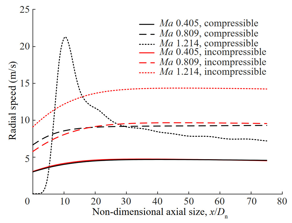Figure  9  Influence of Ma on radial velocity in line A

Download: Full-Size Img

The axial speed at line B (seen in Figure 6) is also displayed in Figure 10, where line B is in the radial direction and the initial point locates at the edge of the cavitator. The maximum axial speed is equal to the flying speed of the supercavitating projectile, and rapidly decreases to an approximate constant value. For the conditions of Ma 0.405 and 0.809, the steady speed is slightly larger than that in incompressible water at the same position. For the conditions of Ma 1.214, the finally speed is about 2 times larger than that in incompressible water. It is demonstrated that the supersonic supercavitating projectile provides stronger disturbance to the flow field because of the existence of underwater shock wave.

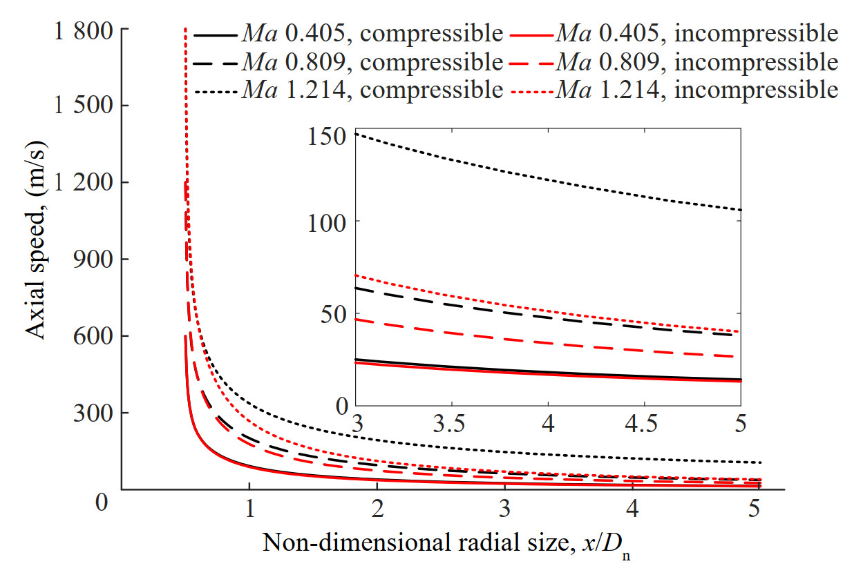Figure  10  Influence of Ma on axial velocity in line B

Download: Full-Size Img

4.2   Supercavity shape

Cavitation number is a non-dimensional parameter used to describe the supercavity shape, and defined as:

where, σ is cavitation number, p_v is the cavitation pressure, ρ_∞ is the density of freestream.

For the calculated cases, the cavitation number changes from 5.4×10⁻³ to 6.6×10⁻⁵, and the full length of the corresponding supercavity is approximately 350D_n – 27 200D_n. The hydrodynamic and motion characteristics are only determined by the supercavity near the projectile (Wang et al. 2020). The length of this part of supercavity is approximately 70D_n. Therefore, only the part of supercavity around the supercavitating projectile is focused.

The contour of the volume fraction of water phase equaling to 0.5 is regarded the boundary of supercavity, and the supercavity profiles are extracted from the numerical results. The outline of supercavity at Ma 1.012 and Ma 1.214 are compared in Figure 11. The axial and radial sizes of the supercavitating projectile and supercavity are normalized by D_n. Moreover, the results from numerical simulations in incompressible water are taken as the reference. The supercavities obtained from the cases with different Ma are approximately the same when the water compressibility is not taken into account. On the contrary, the supercavity size decreases with the increase of Ma if the water compressibility is considered. For the cases with same speed, the water compressibility tends to reduce the radial size of the supercavity near the supercavitating projectile, and the influence further increases with Ma.

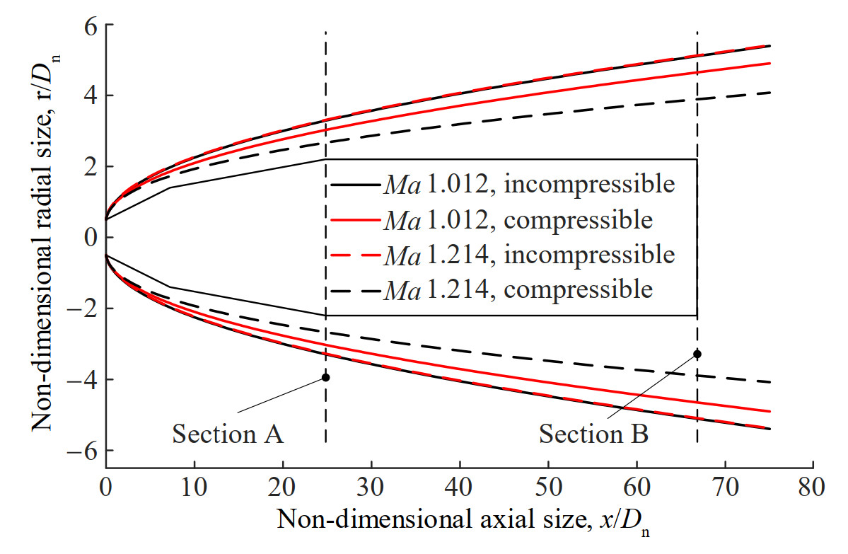Figure  11  Influence of water compressibility on supercavity shape

Download: Full-Size Img

The supercavity profile is roughly a parabola, and can be described by three points (Serebryakov et al., 2009a). The first point related to the supercavity profile is located at the cavitator and its coordinate is (0, 0.5 D_n) as shown in Figure 11. Other two points are also required to fully determine the supercavity. Thus, two cross-sections are selected as characteristic section. The first cross-section (section A) locates at the beginning of the cylinder section of the supercavitating projectile, the other section (section B) is at the tail section of the supercavitating projectile. The positions of section A and section B are displayed in Figure 11. The supercavity diameters at the two sections are quantitatively compared shown in Figure 12.

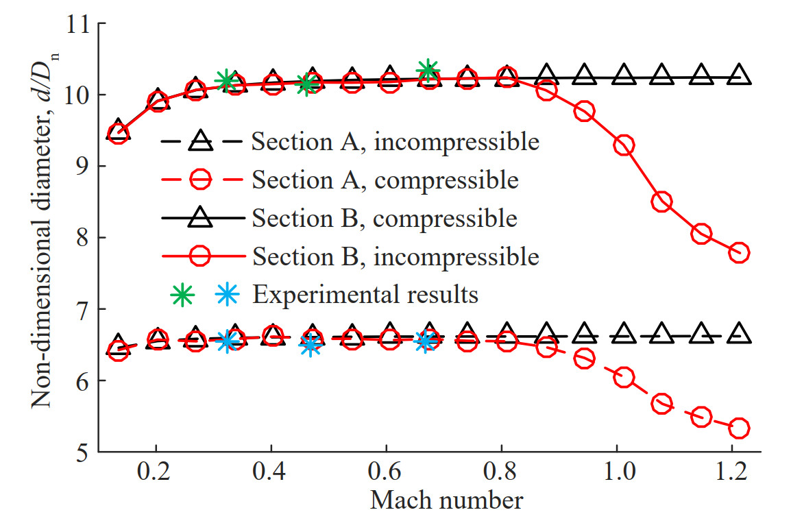Figure  12  Influence of water compressibility and Ma on supercavity size

Download: Full-Size Img

Experimental results of supercavity diameter at the positions of x = 10D_n, 20D_n, 40D_n, 50D_n, 60D_n and 80D_n in the conditions of Ma = 0.331, 0.454, and 0.667 are published (Savchenko et al., 1993). By using the interpolation method, the experiment results at the positions of 25D_n (Section A) and 67D_n (Section B) are obtained, which are compared with the calculation results. The comparison is also displayed in Figure 12. For the three experimental conditions, the relative differences between experimental and numerical results are no more than 3.2% at section A, and no more than 3.8% at section B.

For the cases with speed less than Ma 0.607, the supercavity diameters obtained from incompressible and compressible water are almost the same at both section A and section B. The reason lies in that the compressed extent of water is limited in the low-speed conditions. Then, a tiny difference in the supercavity shape is observed in the range of Ma 0.607–0.809. However, in spite of the speed is same, the supercavity of compressible water is much smaller than that of incompressible supercavity at both section A and section B for the transonic and supersonic conditions. In addition, the difference increases with Ma. The comparison shown in Figure 12 demonstrates that the water compressibility exerts little influence on the supercavity shape near supercavitating projectiles for the subsonic condition, and results in a significant shrinkage of the part of supercavity for the transonic and supersonic conditions.

As described by the principle of independent expansion (Serebryakov, 2009b), the water near the cavitator moving in the radial direction forms a cross-section of supercavity, and overcomes the pressure of far field by consuming the radial moment. The imbalance between radial inertia forces and pressure forces results in the gradually enlarged diameter of the cross-section. The radial speed finally decreases to zero at the point where the diameter of the cross-section expands to the pick value. Thereafter, the pressure from far field forms a reversed radial speed and accelerates gradually, the diameter of the cross-section decreases to zero consequently. In this process, the pick value of the cross-section is the maximum diameter of the supercavity, the flowing distance of the free stream during the existence time of the cross-section is the full length of the supercavity. Therefore, the supercavity shape is determined by both the pressure of far field and radial speed.

As shown in Figures 8 and 9, the static pressure increases and the radial speed decreases in the high-speed conditions when considering water compressibility. It indicates that the kinetic energy forming the supercavity decreases and the resistance preventing the expansion of the supercavity increases in the compressible water. This phenomenon is more obvious in the supersonic conditions. Consequently, the water compressibility significantly shrinks the part of supercavity near supercavitating projectiles in the high-speed condition, especially in the supersonic condition.

To further analyze the effect of water compressibility on the supercavity, the shrinkage ratio of the supercavity at the key section in compressible water is defined as follows.

where, ε is the shrinkage ratio of supercavity, d_i and d_c are the diameter of the compressible supercavity diameter and incompressible supercavity diameter at section A or section B, respectively.

According to the data of Figure 12, the shrinkage ratios at section A and section B at the speed of Ma 0.135–1.214 are calculated in Figure 13. The shrinkage ratios at the two sections are almost zero when the speed is no more than Ma 0.607. When the supercavitating projectile flying with a speed within Ma 0.607–0.809, the water compressibility begins to have slightly influence on the shape of the surrounding supercavity, the maximum shrinkage ratio at section A is about 1.5%, and that of section B is less than 0.5%. For the case of Ma 1.012, the shrinkage ratios at section A and section B are 8.54% and 9.13%, respectively. When the speed is up to Ma 1.214, the shrinkage ratios at the two sections are 19.41% and 23.98%, respectively. To summarize, the shrinkage ratio increases sharply with Ma after the underwater bow shock occurs.

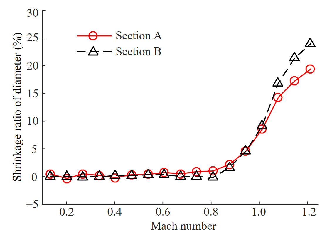Figure  13  Change of shrinkage ratio of supercavity with Ma in compressible water

Download: Full-Size Img

4.3   Hydrodynamic characteristics

The motion characteristic of supercavitating projectiles is determined by the hydrodynamic force. For the calculated conditions, the supercavitating projectile is assumed to fly with no angle of attack and no angle of sideslip, and only subjected to the drag force. Moreover, the supercavitating projectile is fully enveloped by a supercavity, and the drag force only acts on the cavitator. Serebryakov (Serebryakov et al., 2009a) points out that the drag coefficient of the disk cavitator is also related to the pressure coefficient, and the following analytical correlations are proposed.

where, c_* is the pressure coefficient at stagnation point, C_d is the drag coefficient of the disk cavitator.

The drag coefficients of the supercavitating projectile of different speed are obtained by numerical and analytical methods, and compared in Figure 14. The drag coefficient is calculated by dividing the drag by the dynamic pressure of far field. The drag coefficient obtained from compressible water is largely different from that from incompressible water, and this difference increases with Ma. For example, when Ma = 0.135, the drag coefficients are roughly equal between incompressible and compressible water. However, for the case of Ma 1.214, the drag coefficient is increased by 23.90% because of water compressibility. The comparison between numerical simulation in compressible water and theoretical correlations are close, and the relative differences are within 3.5%. It can be seen from Figures 5 – 7 that the stagnation pressure in incompressible water is equal to the sum of the dynamic pressure and static pressure. The dynamic pressure is much larger than the static pressure in the high-speed condition, therefore the drag coefficient is approximately a constant value. However, the water compressibility causes the significant increase of the stagnation pressure, and the increment increases with Ma as shown in Figure 7. Eventually, the drag coefficient of the projectile increases with Ma when water compressibility is taken into account.

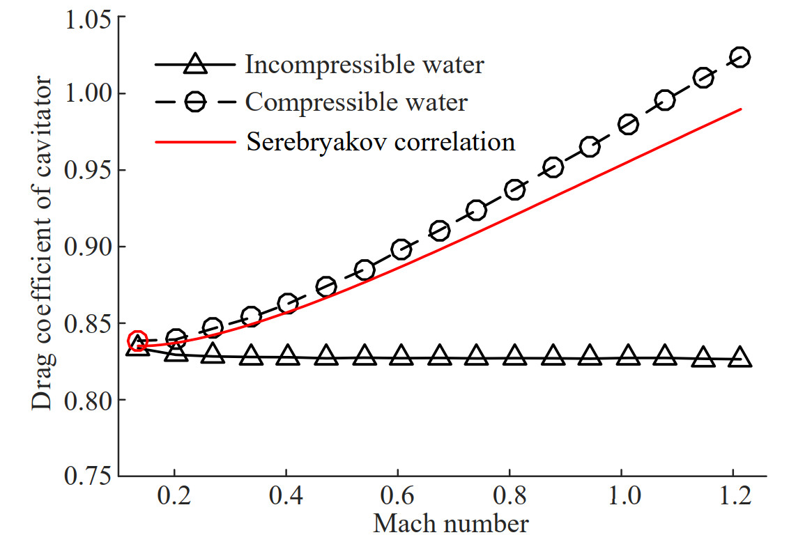Figure  14  Influence of Ma on drag coefficient of disk cavitator

Download: Full-Size Img

When supercavitating projectiles fly in low speed, the compressed extent of water is limited, and the water can be addressed as incompressible fluid. Thus, the value of c_* expressed by Eq. (12) tends to be 1.0, and the drag coefficient of disk cavitator can be regard as 0.827 (1 + σ).Therefore, the drag coefficient is slightly influenced by cavitation number in incompressible water, and the influence is further weakened with the decreases of the cavitation number. The cavitation number decreases from 5.4×10⁻³ to 2.4×10⁻³ when the speed increases from Ma 0.135 to Ma 0.202, and decreases from 2.4×10⁻³ from to 6.6× 10⁻⁵ when the projectile speed increases from Ma 0.202 to Ma 1.214. Therefore, the drag coefficient of the cavitator in incompressible water slightly decreases with the increase of speed, and the change mainly occurs in the range of Ma 0.134 to Ma 0.202.

5   Conclusions

In this paper, numerical simulations are performed to investigate the influence of water compressibility on the subsonic, transonic and supersonic supercavitation flow fields. The flow regime, supercavity shape and hydrodynamic characteristics are compared. The key findings are as follows:

(1) For the supersonic conditions, the water compressibility has significant influences on the distributions of the pressure, radial speed and axial speed, and must be considered. In compressible water, a bow shock is observed in supersonic condition, and a larger stagnation pressure on the disk cavitator is obtained. In addition, the shock changes the distributions of the radial and axial speed of water around supercavitating projectiles.

(2) Water compressibility has no influence on the shape of the part of supercavity near supercavitating projectiles when speed is less than Ma 0.607, leads to a slightly shrinkage of the supercavity in Ma 0.607 – 0.809, and causes a significant shrinkage when speed is more than Ma 0.809. By contrast with the results of incompressible water, the diameter of supercavity at the tail decreases by 9.13% for Ma 1.012, and 23.98% for Ma 1.214.

(3) By considering the water compressibility, the increased stagnation pressure on the disk cavitator results in the increase of drag coefficient comparing with the case of same speed in incompressible water. The drag coefficient increases by 23.90% for the case of Ma 1.214. The calculation change law of drag coefficient with Ma is coincident with the published analytical result.