Research on the Viscoelasticity of Polyester Mooring Lines Using the Absolute Nodal Coordinate Formulation
https://doi.org/10.1007/s11804-022-00273-y
-
Abstract
The taut mooring system using synthetic fiber ropes has overcome the shortcomings such as the large self-weight of the mooring lines and provides better mooring performance for the floating structures. The polyester rope has attracted much attention among numerous synthetic fiber rope materials due to its lightweight, low price, corrosion resistance, and high strength. Thus, the mooring characteristics of it are worth studying. Polyester mooring lines are flexible in deep water, when a marine structure is moored by them, the geometric nonlinearity such as large displacement, large stretch, and large bending deformation, and the material nonlinearity like viscoelastic of the polyester ropes become complex integrated problems to be studied. Considering the nonlinear phenomenon, the simulation and calculation of a polyester line were carried out by the absolute nodal coordinate formulation (ANCF) in this paper since the ANCF method has advantages in dealing with the significant deformation problems of the flexible structures. In addition, a chain mooring line was also simulated for comparison, and the results show that the polyester ropes reduce the self-weight of the mooring lines and provide sufficient mooring strength at the same time, and the nonlinear phenomenon of the polyester ropes is different from that of the chain mooring lines.Article Highlights• The absolute nodal coordinate formulation (ANCF) is more sensitive in capturing the strain of each element, which leads to a difference from the lumped mass method with the mean strain assumption;• A critical value of the motion amplitude was found, making the difference between ANCF and LMM inversed;• The viscoelastic factor affects the hysteresis loop of the polyester rope, and the larger it is, the more obvious the hysteresis effect is. -
1 Introduction
In the field of deepwater exploration and development, the mooring system has brought a series of new problems, such as the suddenly increased weight of the mooring lines, which affects the load weight and motion response of marine structures. Considering this issue from the perspective of economy and security, the taut mooring system composed of synthetic fiber ropes provides a lighter weight, and better mooring performance has been considered more suitable for operation. However, the mechanical properties of synthetic fiber ropes are complex with a robust nonlinear phenomenon, which are different from that of chain cables and steel wires. Many theoretical studies and engineering tests have been carried out with immediate needs in recent years, and compared with other synthetic fiber ropes, polyester cables have become the popular deepwater mooring line because of their excellent characteristics such as good corrosion and fatigue resistance. Francois and Davies (2008) have studied the characterization of polyester mooring lines, including quasi-static stiffness and dynamic stiffness, and relative tests were performed, which provided a model of the visco-elastoplastic response of polyester fiber ropes. Catipovic et al. (2011) have proposed an improved stiffness model using the finite element method, and the highly extensible polyester mooring lines were studied. The conclusions showed that the improved model achieved a better agreement with the analytical results. In addition, a coupled-dynamic analysis of floating structures with polyester mooring lines was carried out (Tahar and Kim, 2008), and the mooring-line dynamics were based on a rod theory and the finite element method with the governing equations described in a generalized coordinate system, and the results indicated that the nonlinearity of polyester ropes was obviously different from linear elastic lines. Ma et al. (2014) have introduced a method for large stretched slender rod theory with the finite element method to deal with the problems of the large rotation and the large deformation, and the rod model works well with the viscoelastic model. Besides, there are a series of researches about fatigue analysis and damage inspections of the polyester ropes (Flory et al., 2006; Beltran and Williamson, 2010), which have provided some engineering references.
In processing the problems of large deformation of structures, Researchers (Berzeri et al., 2001) have proposed the absolute nodal coordinate formulation, which leads to a simple expression for the inertia forces and a nonlinear expression for the elastic forces since the global displacement coordinates and slopes are established in the global coordinate system. Many scholars have applied this formulation in different fields, such as the analysis of composite tires (Patel et al., 2016), the high-order quadrilateral plate (Ebel et al., 2017), and also membrane structures (Zhang et al., 2016), etc. The absolute nodal coordinate formulation can also study polyester mooring lines considering its convenience and efficiency. In this paper, a polyester rope will be modeled, and the nonlinear properties of the rope will be studied by the ANCF method.
2 Absolute nodal coordinate formulation
2.1 Equations of motion
The absolute nodal coordinate formulation defines the nodal element coordinates in a fixed inertial coordinate system, including the global displacement and the slopes. Hence, no transformation matrices are required to define the kinematic position and velocity equations of the elements.
Owing to the large aspect ratio, the deformation of mooring lines is axial stretch and bending. Based on the three-dimensional beam elements of Ahmed et al. (2001) shown in Figure 1, the torsion and shear of mooring lines can be ignored. Thus, an element can be defined as two nodes and twelve absolute nodal coordinates:
$$ \boldsymbol{q}=\left[\begin{array}{llll} q_{1} & q_{2} & \cdots & q_{12} \end{array}\right]^{\mathrm{T}} $$ (1) 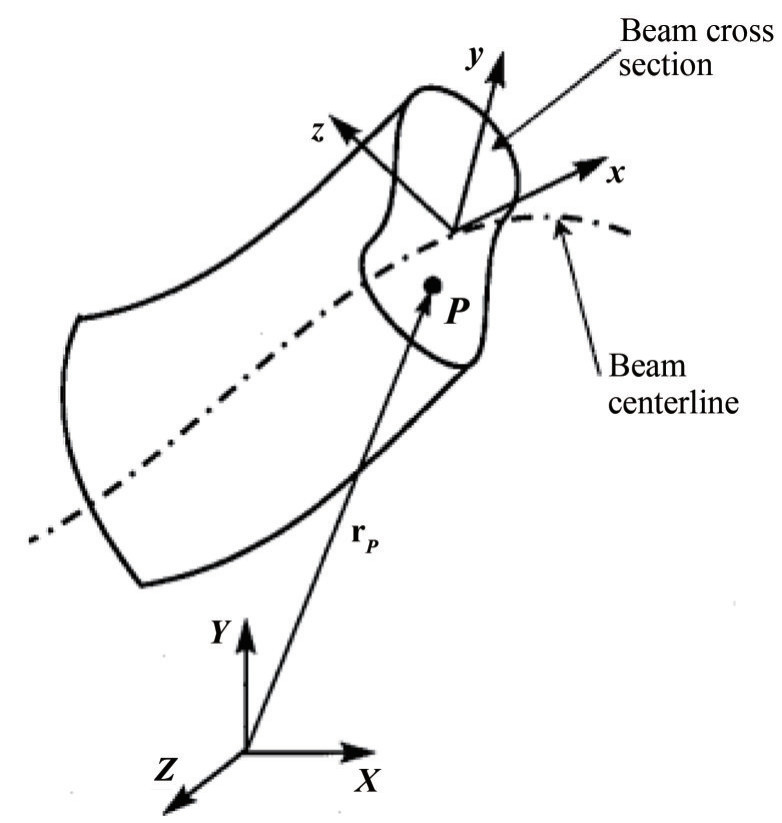 Figure 1 3D beam element model
where q1, q2 and q3 are the displacement terms and q4, q5 and q6 are the slope terms of the left node. Thus, the sagittal diameter of an arbitrary point P on the cross section of a beam element can be defined in the global coordinate system as:
$$ \boldsymbol{r}=\boldsymbol{S q} $$ (2) where S is the element shape function, and Hermite interpolation polynomial was employed here to ensure the continuity of the displacement and slope.
Using the global position vector r defined in Eq. (2), the kinetic energy of the finite element can be defined as (Berzeri et al., 1998; Zhang et al., 2019):
$$ T=\frac{1}{2} \int_{V} \rho \dot{\boldsymbol{r}}^{\mathrm{T}} \dot{\boldsymbol{r}} \mathrm{d} V=\frac{1}{2} \dot{\boldsymbol{q}}^{\mathrm{T}}\left(\int_{V} \rho \boldsymbol{S}^{\mathrm{T}} \boldsymbol{S} \mathrm{d} V\right) \dot{\boldsymbol{q}}=\frac{1}{2} \dot{\boldsymbol{q}}^{\mathrm{T}} \boldsymbol{M} \dot{\boldsymbol{q}} $$ (3) where ρ and V are the mass density and the volume of the element, respectively, and M is the mass matrix defined as (Gerstmayr and Shabana, 2006):
$$ \boldsymbol{M}=\int_{V} \rho \boldsymbol{S}^{\mathrm{T}} \boldsymbol{S} \mathrm{d} V $$ (4) The motion equations can be defined as follows:
$$ \boldsymbol{M} \ddot{\boldsymbol{q}}+\boldsymbol{Q}_{s}-\boldsymbol{Q}_{e}=\bf{0} $$ (5) where Qs is the elastic force and Qe is the externally applied force, and the elastic force Qs can be defined using the strain energy U as (Gerstmayr and Shabana, 2006):
$$ \boldsymbol{Q}_{s}=\left(\frac{\partial U}{\partial \boldsymbol{q}}\right)^{\mathrm{T}}=\int_{0}^{L} E A \varepsilon\left(\frac{\partial \varepsilon}{\partial \boldsymbol{q}}\right)^{\mathrm{T}} \mathrm{d} s+\int_{0}^{L} E I K_{\kappa}\left(\frac{\partial K_{\kappa}}{\partial \boldsymbol{q}}\right)^{\mathrm{T}} \mathrm{d} s $$ (6) The external forces Qe can be defined as:
$$ \boldsymbol{Q}_{e}=\int_{0}^{L}\left(\frac{\partial \boldsymbol{r}}{\partial \boldsymbol{q}}\right)^{\mathrm{T}} \cdot \boldsymbol{f} \mathrm{d} s $$ (7) where f is the generalized external force.
2.2 Viscoelastic force
The viscoelastic force should be employed for synthetic fiber ropes to demonstrate the material nonlinearity. Thus, based on the elastic force defined in Eq. (6), and considering the viscoelastic force (Garcíd et al., 2005), the expression of the supplementary form of Qs is:
$$ \begin{aligned} &\boldsymbol{Q}_{s}=\left(\frac{\partial U}{\partial \boldsymbol{q}}\right)^{\mathrm{T}}=\boldsymbol{Q}_{s 1}+\boldsymbol{Q}_{s 2} \\ &=\int_{0}^{L} E A(\varepsilon+\gamma \dot{\varepsilon})\left(\frac{\partial \varepsilon}{\partial \boldsymbol{q}}\right)^{\mathrm{T}} \mathrm{d} s \\ &+\int_{0}^{L} E I\left(K_{\kappa}+\gamma \dot{K}_{\kappa}\right)\left(\frac{\partial K_{\kappa}}{\partial \boldsymbol{q}}\right)^{\mathrm{T}} \mathrm{d} s \end{aligned} $$ (8) where γ is the viscoelastic damping factor, and the over-dot denotes derivation with respect to time. It should be noted that there are axial strain terms and bending curvature terms in Eq. (8). Since the mooring lines are slender flexible structures, the latter contributes less to the calculation. The derivation of the bending curvature will not be described in detail below.
The axial strain ε and its derivative to q are:
$$ \varepsilon=\sqrt{\boldsymbol{r}^{\prime \mathrm{T}} \boldsymbol{r}^{\prime}}-1 $$ (9) $$ \left(\frac{\partial \varepsilon}{\partial \boldsymbol{q}}\right)^{\mathrm{T}}=\frac{\boldsymbol{S}^{\prime \mathrm{T}} \boldsymbol{r}^{\prime}}{\sqrt{\boldsymbol{r}^{\prime \mathrm{T}} \boldsymbol{r}^{\prime}}} $$ (10) where r' = S'q.
Thus, the strain rate $\dot{\varepsilon}$ is:
$$ \dot{\varepsilon}=\dot{\boldsymbol{q}}^{\mathrm{T}}\left(\frac{\partial \varepsilon}{\partial \boldsymbol{q}}\right)^{\mathrm{T}}=\dot{\boldsymbol{q}}^{\mathrm{T}} \frac{\boldsymbol{S}^{\prime \mathrm{T}} \boldsymbol{r}^{\prime}}{\sqrt{\boldsymbol{r}^{\prime \mathrm{T}} \boldsymbol{r}^{\prime}}} $$ (11) The generalized force in Eq. (8) is composed of the elastic terms and the damping terms. Therefore, Qs1 can also be expressed in the following form:
$$ \boldsymbol{Q}_{s 1}=\boldsymbol{K}_{1} \boldsymbol{q}+\boldsymbol{D}_{1} \dot{\boldsymbol{q}} $$ (12) where K1 and D1 are the stiffness matrix (Lin and Sayer, 2015; Petruska et al., 2005) and damping matrix of the element:
$$ \boldsymbol{K}_{1}=\int_{0}^{L} E A \varepsilon \frac{S^{\prime \mathrm{T}} S^{\prime}}{\sqrt{r^{\prime \mathrm{T}} r^{\prime}}} \mathrm{d} s $$ (13) $$ \boldsymbol{D}_{1}=\int_{0}^{L} E A \gamma\left(\frac{\partial \varepsilon}{\partial \boldsymbol{q}}\right)^{\mathrm{T}} \frac{\partial \varepsilon}{\partial \boldsymbol{q}} \mathrm{d} s $$ (14) 2.3 External force
Assuming that the mooring lines are subjected to uniform gravity and buoyancy, for elements of length ds, the gravity fg and buoyancy fb can be defined as:
$$ \boldsymbol{f}_{g}=-\rho_{m} A_{m} g \boldsymbol{e}_{y} $$ (15) $$ \boldsymbol{f}_{b}=\rho_{s} A_{m} g \boldsymbol{e}_{y} $$ (16) where g is the acceleration of gravity, Am is the circular area of the mooring lines, ρm and ρs are the density of mooring lines and seawater, respectively, ey is the unit vector in the Y direction of the global coordinate system (as shown in Figure 1).
Wave forces acting on a microelement ds can be obtained by the Morison Equation (Kim et al., 2005):
$$ \begin{aligned} &\boldsymbol{f}_{\mathrm{wave}}(s, t)=\frac{1}{2} \rho_{s} C_{d} D \boldsymbol{N}\left(\boldsymbol{v}_{s}-\dot{\boldsymbol{r}}\right)\left|\boldsymbol{N}\left(\boldsymbol{v}_{s}-\dot{\boldsymbol{r}}\right)\right| \\ &+\rho_{s} A_{m}\left(1+C_{m}\right) \boldsymbol{N} \dot{\boldsymbol{v}}_{s}-\rho_{s} A_{m} C_{m} \boldsymbol{N} \ddot{\boldsymbol{r}} \end{aligned} $$ (17) where, Cd and Cm are the drag coefficient and added mass coefficient, D is the diameter of the mooring line, vs and $\dot{\boldsymbol{v}}_{s}$ are the velocity and acceleration of the wave particle, $\dot{\boldsymbol{r}}$ and $\ddot{\boldsymbol{r}}$ are the velocity and acceleration of the mooring line. N is a 3D normal transformation matrix to ensure that the direction of wave force is perpendicular to the mooring line, it is defined as:
$$ \boldsymbol{N}=\boldsymbol{I}-\frac{\boldsymbol{r}^{\prime} \boldsymbol{r}^{\prime \mathrm{T}}}{\boldsymbol{r}^{\prime \mathrm{T}} \boldsymbol{r}^{\prime}} $$ (18) Since the seabed soil force has not been involved in the taut mooring system, and the current force fcurrent(s, t) is also calculated by the Morison Equation, the generalized external force f can be summarized as:
$$ \boldsymbol{f}=\boldsymbol{f}_{g}+\boldsymbol{f}_{b}+\boldsymbol{f}_{\text {wave }}+\boldsymbol{f}_{\text {current }} $$ (19) 3 Key parameters of the mooring line
The properties of the main components of the mooring lines are presented in Table 1. The polyester mooring line has three main components out of the fairlead: top chain, polyester rope, and ground chain.
Table 1 Mooring line configuration and propertiesComponent Diameter(mm) EA(MN) Dry weight(kg/m) Length(m) Fairlead Chain 157 1 960.0 493.0 125.0 Polyester 256 71.4 45.1 1 950.0 Ground Chain 157 1 960.0 493.0 259.0 The water depth of the operation area is about 1 424 m, and the total length of the mooring line is 2 334 m. In addition, the horizontal distance between the fairlead and the anchor point is about 1 916 m.
Aiming to study the dynamic characteristics of the mooring lines, the fairlead will move in a wide range. Thus, the breaking strength of each component has not been given. In addition, the axial stiffness of the polyester rope referred to the average performance of OrcaFlex.
Figure 2 gives the main view of the mooring line, the origin sets on the static position of the fairlead, which is assumed to be fixed on the water surface because the motion of marine structures has not been considered yet in this paper. Instead, a horizontal harmonic motion is set at the fairlead to inspect the dynamic properties of the polyester rope more apparently. The amplitude of the harmonic motion is 5 m, 10 m, 20 m, 30 m, 40 m, and 50 m, respectively, and the circular frequency is 0.2 rad/s with the initial phase − π/2.
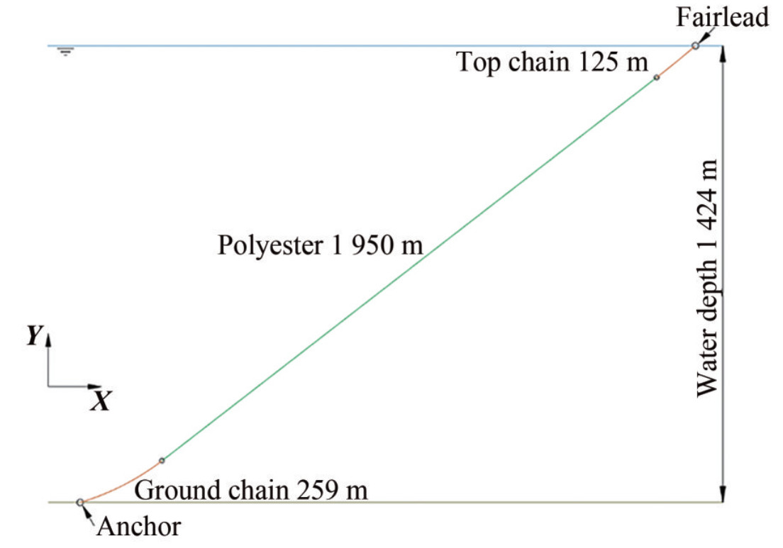 Figure 2 Diagram of the polyester mooring line
4 Results and discussions
4.1 Chain mooring line
The simulation results of the ANCF method have been compared to the OrcaFlex, the theory of which calculating the motions and effective tension of the mooring line is the lumped mass method.
The large magnitude of axial stiffness leads to minor axial strain for the mooring line consisting of the chain cable. Thus, the mean axial strain assumption of the lumped mass method can ensure high precision for the simulation results.
As shown in Figure 3, the solid line represents the static position of the mooring line calculated by the ANCF method, and the dashed line is the simulation results of the lumped mass method. In this case, no external wave and current loads are applied, and the mooring line achieves the static position under the buoyancy and gravity.
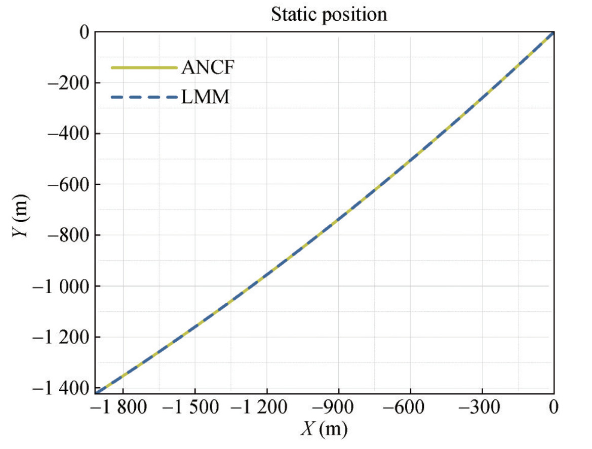 Figure 3 Static position of the chain mooring line
The circular frequency of 0.2 rad/s referred to the motion RAOs of the platform obtained from the frequency domain calculation. To better observe the viscoelastic property, only a single mooring line was simulated in this paper, and the platform with the mooring system was not studied. Finally, we applied this circular frequency on the single polyester rope.
Before calculating the polyester rope, a mooring line only consisting of chains was simulated to verify the applicability of the calculation method. The approach is to replace the polyester rope in Figure 2 with the chain cable, and the detailed parameters of the mooring line are listed in Table 2.
Table 2 Mooring line configuration and propertiesComponent Diameter(mm) EA(MN) Dry weight(kg/m) Length(m) Chain 157 1 960.0 493.0 2 334.0 Apparently, the static position calculated by the ANCF method and the lumped mass method achieves a high agreement. Thus, the initial shape of the mooring line can be considered the same. In addition, Figure 4 displays the effective tension along the mooring line.
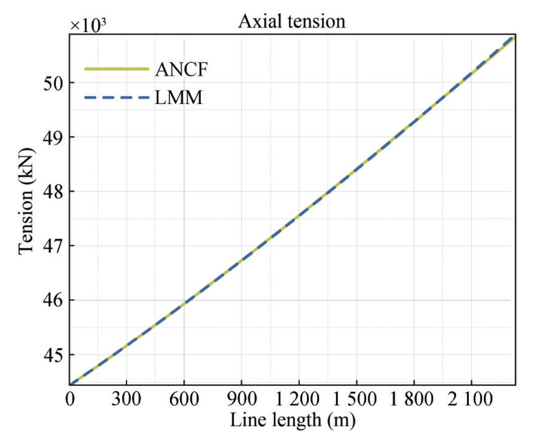 Figure 4 Axial tension along the chain mooring line
At the fairlead, the tension calculated by the lumped mass method is 50 886.91 kN, while the result gained by the ANCF method is 50 862.32 kN, and the error is about 0.048% of the two simulation results. On this basis, the dynamic simulation can be considered comparable.
The dynamic simulation results are shown in Figure 5. The solid lines are the effective tension of the fairlead with different amplitudes of the harmonic motion calculated by the ANCF method. The dashed lines represent the results of the lumped mass method. It should be noted that since the breaking strength (Saidpour et al., 2020; Xu et al., 2021) of the mooring line is not considered in this paper, the effective tension is assumed to be available when the mooring line moves at large amplitudes.
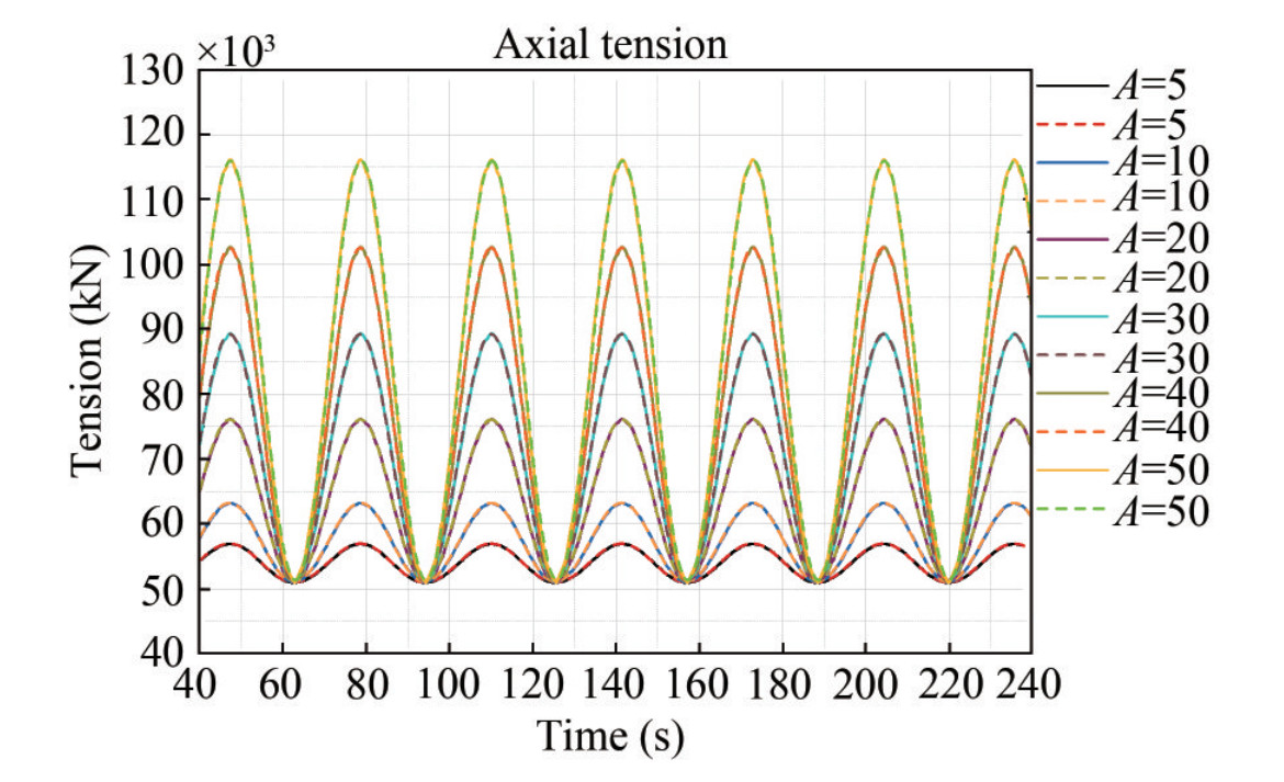 Figure 5 Effective tension of the mooring line in harmonic motion
By comparing the results of the two simulation methods, the effective tension curves agree well, and the error is about 0.05% at the maximum motion amplitude. The results indicate that the dynamic calculation of mooring lines by the ANCF method has high reliability.
4.2 Polyester mooring line
To better observe the difference between the ANCF method and the lumped mass method, the external wave loads and current forces will not be applied.
As mentioned above, the axial stiffness of chain material makes the mean axial strain assumption of the lumped mass method available. Under the large stretch condition, the axial strain of each element is not the same. The calculation results of averaging the large strains generated by local elements to the entire mooring line may be distorted. Thus, the mechanical properties of mooring lines such as polyester ropes may be quite different.
In the following, the ANCF method will be employed to study the mechanical properties of polyester ropes under the large stretch circumstance. Based on the comparison results of the chain mooring line, the same approach will be used to study the mooring characteristics of polyester ropes. Due to the difference in material properties, the mean strain assumption may cause some errors in the calculation results.
As shown in Figure 6, the static position of the polyester mooring line is also roughly the same under the two calculation methods. Nonetheless, there is a tiny difference near the anchor point, which is that the position gained by ANCF is lower by about 7 meters than that of the lumped mass method. Owing to the enormous gravity of the ground chain, the axial strain of the polyester rope is relatively large at the connection of the ground chain and polyester line. Subsequently, the large stretch of polyester rope makes the ground chain reach a static equilibrium at a lower position. However, the mean axial strain assumption averages the strain in each polyester element so that the static position of the line is high.
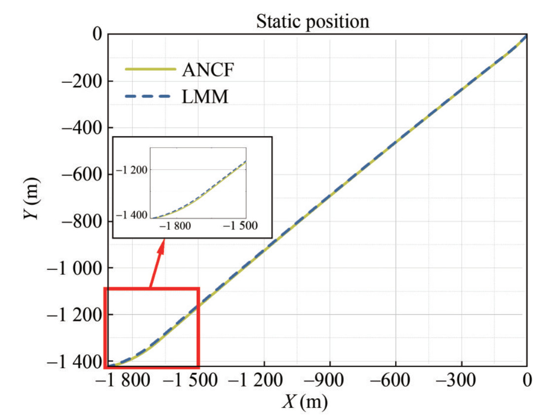 Figure 6 Static position of the polyester mooring line
Meanwhile, the tension of the fairlead obtained from the lumped mass method is 2 623.67 kN, while the result of the ANCF method is 2 598.19 kN, and the error of the effective tension at the fairlead is about 0.98% (Figure 7), which ensures that the comparison of the dynamic calculations is credible.
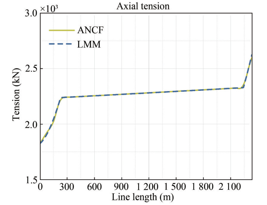 Figure 7 Axial tension along the polyester mooring line
To observe the difference in the effective tension carried out by the two methods, Figure 8 presents the tension of the fairlead under different amplitudes of the harmonic motion respectively.
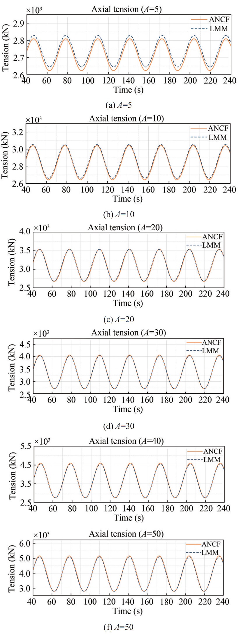 Figure 8 Effective tension of the polyester mooring line
For the same mooring line, the axial strain of polyester rope should be more significant than that of the chain. As shown in Figures 8(a) and 8(b), the simulation results of the ANCF method are smaller than that of the lumped mass method. This phenomenon is because ANCF captures the axial strain of each element. When the amplitude of harmonic motion is small (such as A = 5 m and A = 10 m), the axial elongation of the top chain is mainly at the connection between the two mooring materials. However, the mean strain assumption averages the elongation to each element of the chain so that the effective tension of the lumped mass method is large.
In Figure 8, the max axial tension is almost the same, which indicates that the displacement of the fairlead makes the strain of the top chain also large. The strain is almost equivalent to that caused by the stress of the polyester rope on the top chain. Thus, the effective tension obtained by the two calculation methods is close to each other.
Furthermore, it seems like there is a critical value of the amplitude. When the amplitude of harmonic motion exceeds it, the axial tension of the ANCF method is more significant than that of the LMM. Under a large amplitude of over 30 m, the axial elongation of the fairlead chain captured by ANCF should be more prominent. However, the LMM averages the elongation in each element so that the axial tension is small.
Combined with the analysis above, Figure 9 shows the maximum axial tension and the difference at each amplitude of the harmonic motion. The bar chart represents the tension, and the line graph shows the difference. In addition, the percentage of the difference is also marked. As amplitude increases, the maximum axial tension difference between ANCF and LMM increases from small to large, and there is indeed a critical point that makes the two calculations equal. In general, the effective tension error obtained by the two methods is still small in the calculation of the mooring line model in this paper.
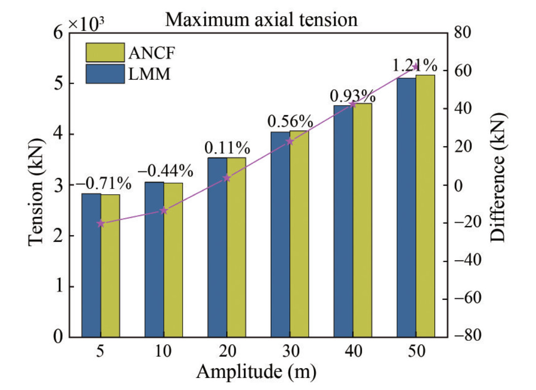 Figure 9 Maximum effective tension and the difference
4.3 Influence of the damping coefficient
The damping factor γ defined in Eq. (8) is an important parameter that affects the viscoelasticity of the polyester rope. In the above simulation results, γ considered to be 0.1, the coefficient depends on the hysteresis effect of materials (Garcíd et al., 2005). In this section, to study the hysteresis phenomenon (Lian et al., 2019; Huang et al., 2013; Liu et al., 2014) of polyester rope, three different damping coefficients will be calculated, and the simulation results will be compared and analyzed.
As shown in Figure 10, the solid lines, dashed lines, and dot lines present that γ =0.5, 0.1, and 0.01, respectively, the amplitudes of the harmonic motion are the same as above, and the details of the curves are enlarged in the red frame. By comparing Figure 5 and Figure 10, the obvious phenomenon is that the valley value of the harmonic curve of polyester rope is not equal, which indicates that the viscoelasticity of the polyester rope does affect the effective tension of the mooring line. The effective tension of linear elastic material such as the chain in Figure 5 is also linear with the displacement of the fairlead. However, when the fairlead of the polyester mooring line reaches the point with the minimum displacement from a distance, the effective tension is not the same under different amplitudes, mainly because of the hysteresis relationship between the stress and strain of polyester rope.
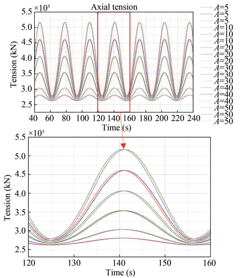 Figure 10 Effective tension of the polyester mooring line with different γ
The hysteresis phenomenon will be analyzed in detail in the following, combined with the enlarged view in Figure 10. Firstly, one obvious piece of information that can be reflected in the figure is that the larger γ it is, the earlier the curve reaches the maximum value, which indicates that the hysteresis increases with the increase of γ. When the displacement increases, the ratio of stress to strain exceeds the dynamic stiffness, which means that the effective tension will increase rapidly, and the growth rate decreases with the increase of displacement and reaches the maximum value. For example, when the amplitude of the harmonic motion is 50 m γ = 0.5, the effective tension is larger than the other two at the same point in time. On the contrary, during the process that the displacement decreases, the effective tension will decline rapidly. However, it will not go back to the initial value of the static condition, which explains that the minimum effective tension does not equal each other under different amplitudes.
5 Conclusions
In this paper, a chain mooring line and a polyester mooring line were modeled and simulated by ANCF, and the calculations were compared to the same model under LMM. The main conclusions can be summarized as follows:
1) Under the small-strain condition, the ANCF model reaches high precision compared to the LMM by OrcaFlex software, which provides a reliable foundation for calculating the immense strain.
2) The material nonlinearity of polyester rope makes the results of ANCF different from those of LMM, and the former is more sensitive in capturing the strain of the element. The mean strain assumption of LMM leads to some errors in calculating the effective tension.
3) The viscoelastic factor affects the hysteresis loop of the polyester rope, and the larger it is, the more obvious the hysteresis effect is. In engineering practice, the viscoelastic factor can be obtained by some experiments and measurements to get a more reliable value.
-
Figure 1 3D beam element model
Figure 2 Diagram of the polyester mooring line
Figure 3 Static position of the chain mooring line
Figure 4 Axial tension along the chain mooring line
Figure 5 Effective tension of the mooring line in harmonic motion
Figure 6 Static position of the polyester mooring line
Figure 7 Axial tension along the polyester mooring line
Figure 8 Effective tension of the polyester mooring line
Figure 9 Maximum effective tension and the difference
Figure 10 Effective tension of the polyester mooring line with different γ
Table 1 Mooring line configuration and properties
Component Diameter(mm) EA(MN) Dry weight(kg/m) Length(m) Fairlead Chain 157 1 960.0 493.0 125.0 Polyester 256 71.4 45.1 1 950.0 Ground Chain 157 1 960.0 493.0 259.0 Table 2 Mooring line configuration and properties
Component Diameter(mm) EA(MN) Dry weight(kg/m) Length(m) Chain 157 1 960.0 493.0 2 334.0 -
Ahmed A, Shabana Refaat Y, Yakoub (2001) Three dimensional absolute nodal coordinate formulation for beam elements: theory. Journal of Mechanical Design 123(4): 614-621. https://doi.org/10.1115/1.1410100 Beltran J, Williamson E (2010) Numerical Simulation of damage localization in polyester mooring ropes. Journal of Engineering Mechanics 136(8): 945-959 https://doi.org/10.1061/(ASCE)EM.1943-7889.0000129 Berzeri M, Campanelli M, Shabana AA (1998) Definition of the Elastic Forces in the Finite Element Formulations. Technical Report OMB No. 0704-0188 Berzeri M, Campanelli M, Shabana AA (2001) Definition of the elastic forces in the finite-element absolute nodal coordinate formulation and the floating frame of reference formulation. Multibody System Dynamics 5(1): 21-54. https://doi.org/10.1023/a:1026465001946 Catipovic I, Coric V, Radanovic J (2011) An improved stiffness model for polyester mooring lines. Brodogradnja 62(3): 235-248 https://hrcak.srce.hr/72269 Ebel H, Matikainen M, Hurskainen V, Mikkola A (2017) Analysis of high-order quadrilateral plate elements based on the absolute nodal coordinate formulation for three-dimensional elasticity. Advances in Mechanical Engineering 9(6): 1-12. https://doi.org/10.1177/1687814017705069 Flory J, Banfield S (2006) Durability of polyester ropes used as deepwater mooring lines. OCEANS 2006 48: 1-5. https://doi.org/10.1109/OCEANS.2006.306947 Francois M, Davies P (2008) Characterization of polyester mooring lines. OMAE 2008: Proceedings of the 27th International Conference on Offshore Mechanics and Arctic Engineering 1: 169-177. https://doi.org/10.1115/OMAE2008-57136 Garcíd D, a-Vallejo, Valverde J, Domínguez J (2005) An Internal Damping Model for the Absolute Nodal Coordinate Formulation. Nonlinear Dynamics 42(4): 347-369. https://doi.org/10.1007/s11071-005-6445-1 Gerstmayr J, Shabana AA (2006) Analysis of thin beams and cables using the absolute nodal co-ordinate formulation. Nonlinear Dynamics 45(1): 109-130. https://doi.org/10.1007/s11071-006-1856-1 Huang W, Liu H, Lian Y, Li L (2013) Modeling nonlinear creep and recovery behaviors of synthetic fiber ropes for deepwater moorings. Applied Ocean Research 39: 113-120. https://doi.org/10.1016/j.apor.2012.10.004 Kim M, Koo B, Mercier R, Ward E (2005) Vessel/mooring/riser coupled dynamic analysis of a turret-moored fpso compared with otrc experiment. Ocean Engineering 32(14-15): 1780-1802. https://doi.org/10.1016/j.oceaneng.2004.12.013 Lian Y, Liu H, Yim S, Zheng J, Xu P (2019) An investigation on internal damping behavior of fiber rope. Ocean Engineering 182(JUN.15): 512-526. https://doi.org/10.1016/j.oceaneng.2019.04.087 Lin Z, Sayer P (2015) An enhanced stiffness model for elastic lines and its application to the analysis of a moored floating offshore wind turbine. Ocean Engineering 109(15): 444-453. https://doi.org/10.1016/j.oceaneng.2015.09.002 Liu H, Huang W, Lian Y (2014) An experimental investigation on nonlinear behaviors of synthetic fiber ropes for deepwater moorings under cyclic loading. Applied Ocean Research 45(45): 22-32. https://doi.org/10.1016/j.apor.2013.12.003 Ma G, Sun L, Wang H (2014) Implementation of a Visco-Elastic Model Into Slender Rod Theory for Deepwater Polyester Mooring Line. American Society of Mechanical Engineers. Volume 8A: Ocean Engineering https://doi.org/10.1115/OMAE2014-23594 Patel M, Orzechowski G, Tian Q, Shabana AA (2016) A new multibody system approach for tire modeling using ANCF finite elements. Proceedings of the Institution of Mechanical Engineers Part K-Journal of Multi-Body Dynamics 230(1): 69-84. https://doi.org/10.1177/1464419315574641 Petruska D, Geyer J, Macon R, Craig M, Ran A, Schulz N (2005) Polyester mooring for the mad dog spar—design issues and other considerations. Ocean Engineering 32(7): 767-782. https://doi.org/10.1016/j.oceaneng.2004.10.002 Saidpour H, Li L, Vaseghi R (2020) The effect of rope termination on the performance of polyester mooring ropes for marine applications. Ocean Engineering 195: 106705. https://doi.org/10.1016/j.oceaneng.2019.106705 Shabana AA (1997) Definition of the slopes and the finite element absolute nodal coordinate formulation. Multibody System Dynamics 1(3): 339-348. https://doi.org/10.1023/A:1009740800463 Tahar A, Kim M (2008) Coupled-dynamic analysis of floating structures with polyester mooring lines. Ocean Engineering 35(17-18): 1676-1685. https://doi.org/10.1016/j.oceaneng.2008.09.004 Xu S, Wang S, Soares CG (2021) Experimental study of the influence of the rope material on mooring fatigue damage and point absorber response. Ocean Engineering 232(13): 108667. https://doi.org/10.1016/j.oceaneng.2021.108667 Zhang C, Kang Z, Ma G, Xu X (2019) Mechanical modeling of deepwater flexible structures with large deformation based on absolute nodal coordinate formulation. Journal of Marine Science and Technology 24: 1241-1255. https://doi.org/10.1007/s00773-018-00621-0 Zhang Y, Liu R, Guo H, Deng Z, Zhao H (2016) Analysis of mechanical properties for membrane structure by the absolute nodal coordinate formulation. IEEE International Conference on Mechatronics and Automation, 1262-1267. https://doi.org/10.1109/ICMA.2016.7558743