1   Introduction

Water entry of structures, as a fundamental and widely concerned mechanical issue, is tightly related to many applications in engineering. In particular, water entry problems are frequently encountered in ocean engineering applications, e.g. free-fall of lifeboats (Huang et al., 2021), launching of torpedoes from air, aircraft ditching (Woodgate et al., 2019; Xiao et al., 2017), ship slamming (Cheng et al., 2020), etc. To ensure safety of marine vehicles, the physical characteristics of the marine structure after water entry should be well studied and understood, including the velocity and acceleration variation of the structure, the pressure loaded on the structure surface and the fluid splashing induced by the strong impact (Lin, 2007).

The first significant study of water entry was conducted by Von Karman and Wattendorf (1929) who estimated the slamming forces on wedges according to conservation of fluid-wedge momentum theory and the added mass effect, which was applied to predict the maximal pressure estimation on the floats of hydroplanes during sea landings. Wagner (1932) also investigated a similar issue for the impact of objects on liquid surfaces. Later, based on the velocity potential theories, Dobrovol'skaya (1969) investigated a two-dimensional wedge water entry problem. However, in these theories, the water entry models were limited to ideal conditions so that it is not enough to reflect the real water entry process of marine structures with complex shapes considering the effects of air phase and fluid compressibility. After that, numerous experimental studies were reported on the water entry of the various axisymmetric shapes. For example, the experiment by Moghisi and Squire (1981) reported the initial impact force on a sphere striking a liquid surface. The study of Lin and Shieh (1997) provided experimental data for impact pressure and the acceleration of structures with circular cylindrical shapes. Yettou et al. (2006) investigated the pressure distribution on a free-falling wedge upon entering water experimentally. Especially, Truscott and Techet (2009) investigated experimentally the water entry of both spinning and non-spinning spheres at low Froude numbers. In particular, Aristoff et al. (2010) combined experimental and theoretical methods to predict the sphere dynamics. Indeed, the experimental tests provide plenty of reliable results to conclude the mechanism of water entry problems. However, due to the limitations of expensive cost and long experimental duration, the experimental method is not efficient, convenient and simple to investigate the water entry issues. To foster the research on alternative methods, more computational fluid dynamics (CFD) solvers are developed which can avoid the high expense in experiments and simulate more complex conditions compared to analytical models (Zhao and Faltinsen, 1993; Yu et al., 2015). Using the Eulerian mesh-based solvers, Iranmanesh and Passandideh-Fard (2017) investigated the water entry of a horizontal circular cylinder in three dimensions (3D), tracking the free surface using the VOF method. In addition, detailed studies on water entry problems were carried by Van Nuffel et al. (2014); Wang and Soares (2020); Wang et al. (2021); Wang and Soares (2022). As mentioned before, the treatment of free surface is complicated for grid-based Eulerian methods. Further, the sharpness of free surfaces could be lost in the space where the mesh resolution is not fine enough. In contrast, the mesh-free method or particle method owns significant advantages for such problems with splashing free surface.

Smoothed particle hydrodynamics (SPH) method, thanks to its Langrangian feature, is capable of dealing with the free surface breaking and water splashing (Yang et al., 2020), demonstrating that the SPH is a competitive method for ocean engineering applications, see Ye et al. (2019); Liu and Zhang (2019); He et al. (2020); Long et al. (2021); Luo et al. (2021); Sun et al. (2021a); and Lyu et al. (2022a). Actually, extensive SPH simulations were accomplished for the water entry problems, see Shao (2009); Skillen et al. (2013a); Khayyer and Gotoh (2016); Gong et al. (2016); Zhang et al. (2017); Sun et al. (2018); and Wang et al. (2019). The authors simulated the water entry of rigid bodies including wedge, sphere and plate using weakly-compressible (see e. g. Oger et al. (2006); Vandamme et al. (2011); and Omidvar et al. (2012)) or incompressible SPH models (Shao and Gotoh, 2004; Bøckmann et al., 2012; and Skillen et al., 2013b). However, most of the SPH simulations are limited to two dimensions (2D). Further, most investigations were performed with single-phase SPH model, neglecting the effect of air. For some fluid impact problems, the air phase has a significant influence on the flow evolution and the slamming load on structures. To simulate multiphase flows, SPH has been proved to be an excellent method (Colagrossi and Landrini, 2003; Hammani et al., 2020) thanks to its advantage of tracking the particles in a Lagrangian fashion, and therefore, the interface between two phases can be straightforwardly captured. In that way, the water entry process can be simulated accurately.

Importantly, as highlighted in Marrone et al. (2017), the water entry simulation using SPH in 3D would lead to enormous computational cost, so that it is challenging for engineering applications. From this aspect, for some axisymmetric problems, SPH simulation in the cylindrical coordinate system can be applied to save the computational cost. Ming et al. (2014) adopted an axisymmetric SPH model to study underwater explosion problems. Brookshaw (2003) proposed an axisymmetric SPH discretization in the cylindrical coordinate, while their model has an obstacle to treating with the axis singularity. Recently, Gong et al. (2019) developed an axisymmetric SPH model under the weakly-compressible assumption for water entry problems. For the above-mentioned axisymmetric SPH studies, the treatment of the symmetric axis is not easy due to the singularity which could lead to problems of numerical instability. Recently, Sun et al. (2021b) adopted the ghost particles mirrored on the other side of the axis, avoiding axis singularities and, further, they proposed a Volume Adaptive Scheme (VAS) to keep uniform particle distributions with homogeneous volumes. Later, Fang et al. (2022) extended this technique to the framework of Riemann-SPH, and investigated different multiphase flows with complex interfaces. In the above studies, the axisymmetric SPH model has been applied to water entry problems, but in their works the axisymmetric SPH simulations were mainly applied to predict the motions of the structure, without carefully validating the local impact pressure which will be carried out in the present work. In addition, the particle resolution was not fine enough in previous studies and therefore the splashing jets were not captured accurately.

In the present work, an axisymmetric SPH method is implemented for different water entry problems with different structures, including sphere and cones with different deadrise angles. Similar to Sun et al. (2021b), the VAS is applied to ensure the homogeneousness of the particle volumes. To investigate the water entry problems more comprehensively, the local impact pressure will be carefully validated and discussed after a convergence study. In addition, the slashing jets are captured and carefully compared with experimental snapshots.

The paper is arranged as follows: Section 2 introduces the axisymmetric SPH model, the treatment of singularity at axis, the volume adaptive scheme and the boundary conditions. Section 3 displays results of water entry simulations validated with experiment data, demonstrating the accuracy and advantages of the axisymmetric SPH model after convergence analysis. Finally, Section 4 gives concluding remarks and perspectives regarding the SPH simulation of water entry in the present work and in the future studies.

2   Axisymmetric SPH model

2.1   Governing equations and axisymmetric simplification

To simulate the water entry problems, similar to the previous studies (Lyu et al., 2021; Gong et al., 2016), the fluid is assumed to be inviscid and weakly-compressible. Grounded on these assumptions, the governing equations in cylindrical coordinates (Gong et al., 2019) are presented as follows:

in which ρ and p represent density and pressure, respectively. The v^r, v^θ and v^z denote the three components of the velocity vector v in the radial(r), circumferential (θ) and axial (z) directions, respectively. g^z is the magnitude of the gravity acceleration in the z direction. The first equation in Eq. (1) represents the continuity equation and other three equations are the components of momentum equation described in three dimensional coordinates (r-θ-z).

Under the axisymmetric assumption, the circumferential velocity component v^θ=0 and the partial derivative of pressure ∂p/∂θ=0 (Sun et al., 2021b). The governing equations in Eq. (1) can be simplified as follows:

Therefore, the water entry problems can be simplified by reducing the problem to an axisymmetric one, see Figure 1.

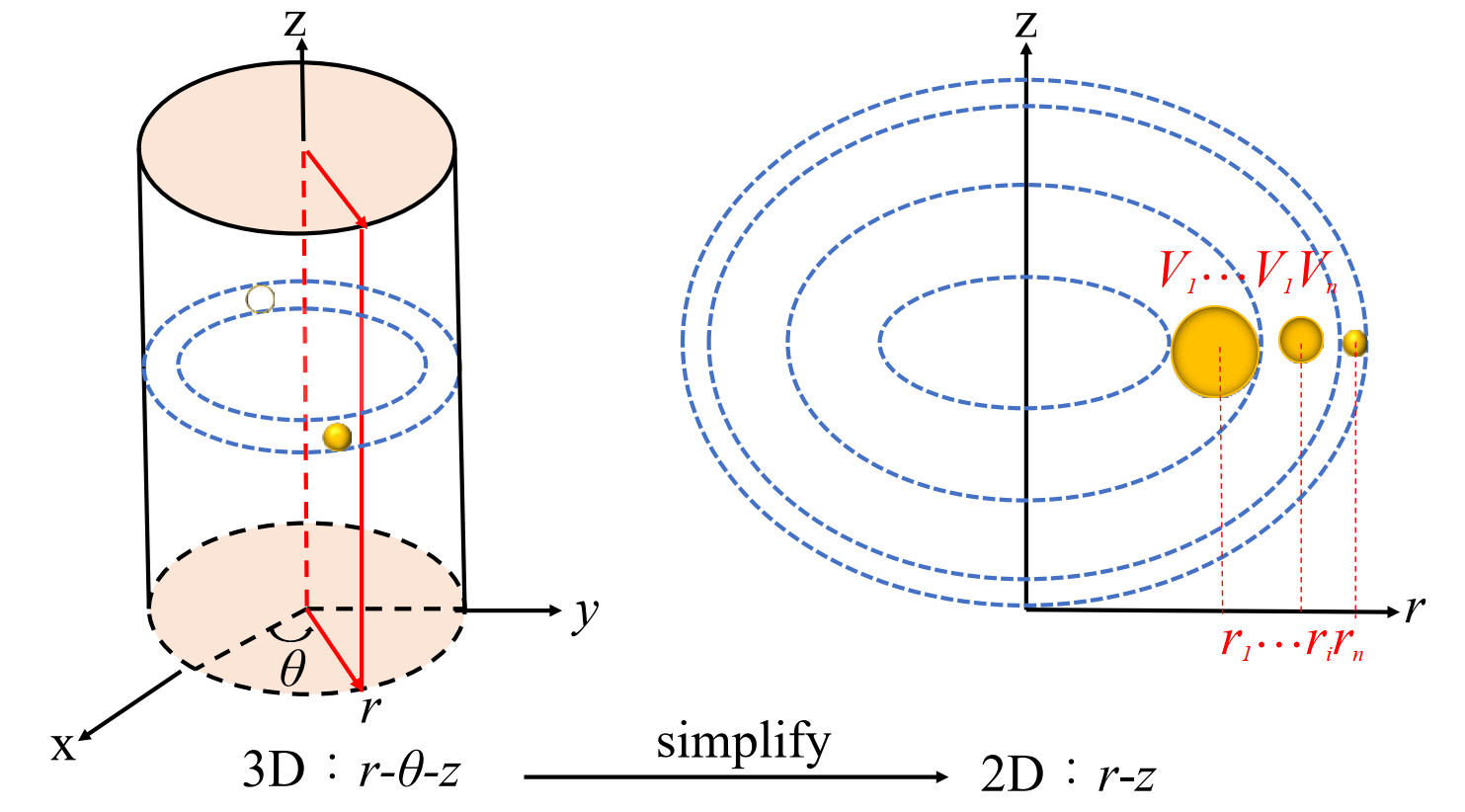Figure  1  The diagram showing the simplification from a 3D cylindrical coordinates system to a 2D axisymmetric plane. In the 2D plane on the right side, the particle mass m_i is equal to the torus mass in the 3D cylindrical coordinate system, which should be conserved in the flow evolution unless a particle splitting or coalescing occurs. Therefore, the particle volume V_i varies directly when the radial coordinate r_i changes (Sun et al., 2019)

Download: Full-Size Img

2.2   Discretizations

The water entry of axisymmetric body can be simulated using the axisymmetric SPH model with particles only distributed in r-z plane, thus straightforwardly avoiding the enormous number of fluid particles needed in the purely 3D SPH simulations. The governing equations (Eq. (2) (Sun et al., 2021b)) are discretized as

where the subscript i denotes the i-th particle and j denotes the particles in the kernel supporting region of i. v and g have components in two directions, denoted as v = (v^r, v^z) and g=(0, −g^z). ρ_ij is denoted as (ρ_i + ρ_j)/2. W_ij represents the kernel function for which the Wendlend C2 kernel is used in this work. The smoothing length is set to h = 2Δx where Δx denotes the particle spacing. r_i is the vector of particle position of particle i. For the sake of stabilizing the density/pressure and velocity fields, the diffusive terms with D_ij and π are added in governing equations(Antuono et al., 2010, 2012). The constant parameter δ = 0.1 is used in the density diffusive term. D_ij is defined as follows:

in which

where < ▽ρ > _i^L and < ▽ρ > _j^L represent the renormalized density gradient (Randles and Libersky, 1996), and r_i represents the position vector of particle i. The viscous term π_ij is given as

where, to ensure numerical stability, the constant parameter α=0.05 is used for water, α=0.3 is used for air and c_ij= (c_i + c_j)/2. Further, to regularize the particle distribution, the particle shifting technique (PST) is adopted. More details can be seen in Sun et al.(2019, 2021b).

Finally, the velocity divergence < ▽· v > ^L1, density gradient < ▽ρ > ^L1 and pressure gradient < ▽p_i > ^L2 are discretized similar to Sun et al. (2021b), written as

In addition, the technique of Tensile Instability Control is applied to reformulate the pressure gradient term to prevent the tensile instability when the pressure becomes negative, more details see Sun et al. (2017).

2.3   The equation of state

In order to obtain the pressure of fluid particles, the equation of state is applied to link the density and pressure (Colagrossi and Landrini, 2003), written as:

where c₀ is the artificial sound speed and ρ₀ is the reference density when the particle pressure is equal to the background pressure p₀. For water entry problems, the air and water phase are both taken into consideration. The pressure for two phases is calculated with Eq. (8). In the multi-phase SPH model, following Colagrossi and Landrini (2003), the polytrophic coefficient γ is set as γ_w =7 for water and γ_a=1.4 for air. To satisfy the weakly-compressible assumption, in the water phase, the density variation should be less than 1% of ρ₀, i.e. ρ/ρ₀ < 1%. In order to meet this requirement, the artificial sound speed c_0w of water is constrained by the maximum expected pressure p_max and velocity v_max (Sun et al., 2017), written as

As for the gas phase, the speed of sound c_0a (Sun et al., 2021) is given as

In all the SPH simulations, the reference density of water is set as 1 000 kg/m³ while the one of air is set as 1.29 kg/m³. It leads to a larger sound speed in the air phase, reducing the time step and therefore making the computational cost of multiphase SPH simulations very expensive. But in this work, thanks to the axisymmetric SPH model, the 3D problem can be simulated in a 2D plane, therefore particle numbers are significantly reduced. In addition, the fourth-order-Runge-Kutta format is implemented to integrate the governing equations (Sun et al., 2021b). The time step is determined by:

where the sound speed c₀ is selected using the maximum value between c_0a and c_0w, and the CFL number is set as 0.5. Constrained by the above condition, the time step in simulations is small enough to keep stability. Recently, He et al. (2022) proposed a stable multiphase SPH model with a larger CFL number which could further improve the numerical efficiency.

2.4   Treatment of symmetry axis

In the present axisymmetric SPH scheme, the treatment of the symmetry axis is an essential but challenging problem. Firstly, the particles close to the axis (r ➝ 0) would lack neighbor particles in the domain of r < 0, resulting in the truncated kernel support. Further, the calculation of 1/r_i in governing equations (Eq.(3)) at the axis, i.e. r➝0, would lead to numerical singularity. To solve this problem, on the other side of the axis (i.e. r < 0) and within a distance of 2 h, ghost particles are created based on mirroring the fluid particles with respect to the axis. Noting that the velocity of ghost particles takes the same value of the fluid velocity in the z-direction, but takes the opposite value in the r-direction. The other physical quantities of ghost particle are directly copied from the corresponding fluid particles (Sun et al., 2021b). Finally, quantities of the ghost particles are given as

where the subscript g and f represent the ghost particles and fluid particles, respectively. In fact, the calculation of SPH divergence and gradient operators in Eq. (7) is not affected by the term 1/r. Further, with the ghost particles, the fluid particles are bounced back when they are about to penetrate the axis. Therefore, the singularity at the axis can be naturally avoided, guaranteeing the numerical stability.

2.5   Volume adaptive scheme (VAS)

Thanks to the Lagrangian properties of SPH model and especially in the axisymmetric SPH model, each fluid particle represents a fluid torus in the 3D space. When simplifying from 3D space to the 2D r-z plane, as shown in Figure 1, each particle volume in 2D represents the cross-section of the fluid torus (Sun et al., 2021b), written as

which indicates that the particle volume varies with the distance to the axis r_i(t). Therefore, to limit the range of the volume variation, the VAS proposed by Sun et al.(2021, b) is implemented in the current work.

Limitation of the volume variation is realized with particle splitting and merging. Particle splitting is triggered when its volume is too large, while particle merging is triggered when its volume is too small, which aims to avoid clustered or sparse particle distributions. The process of VAS is shown in Figure 2. The step of splitting or merging is determined by the ratio between the real-time particle volume and the reference one. Specifically, if the particle volume V exceeds V_max (restriction on particle growing), the mother particle will be split into four daughter particles distributed on the vertices of a square (Sun et al., 2021b), assigned with the particle volume of V_max/4. As aforementioned, the VAS scheme is designed to homogenize particle distribution, guaranteeing the volume variation in a small range. That means the volume variation before splitting is equal to the volume variation after splitting (Sun et al., 2021), i.e. satisfying the following relation:

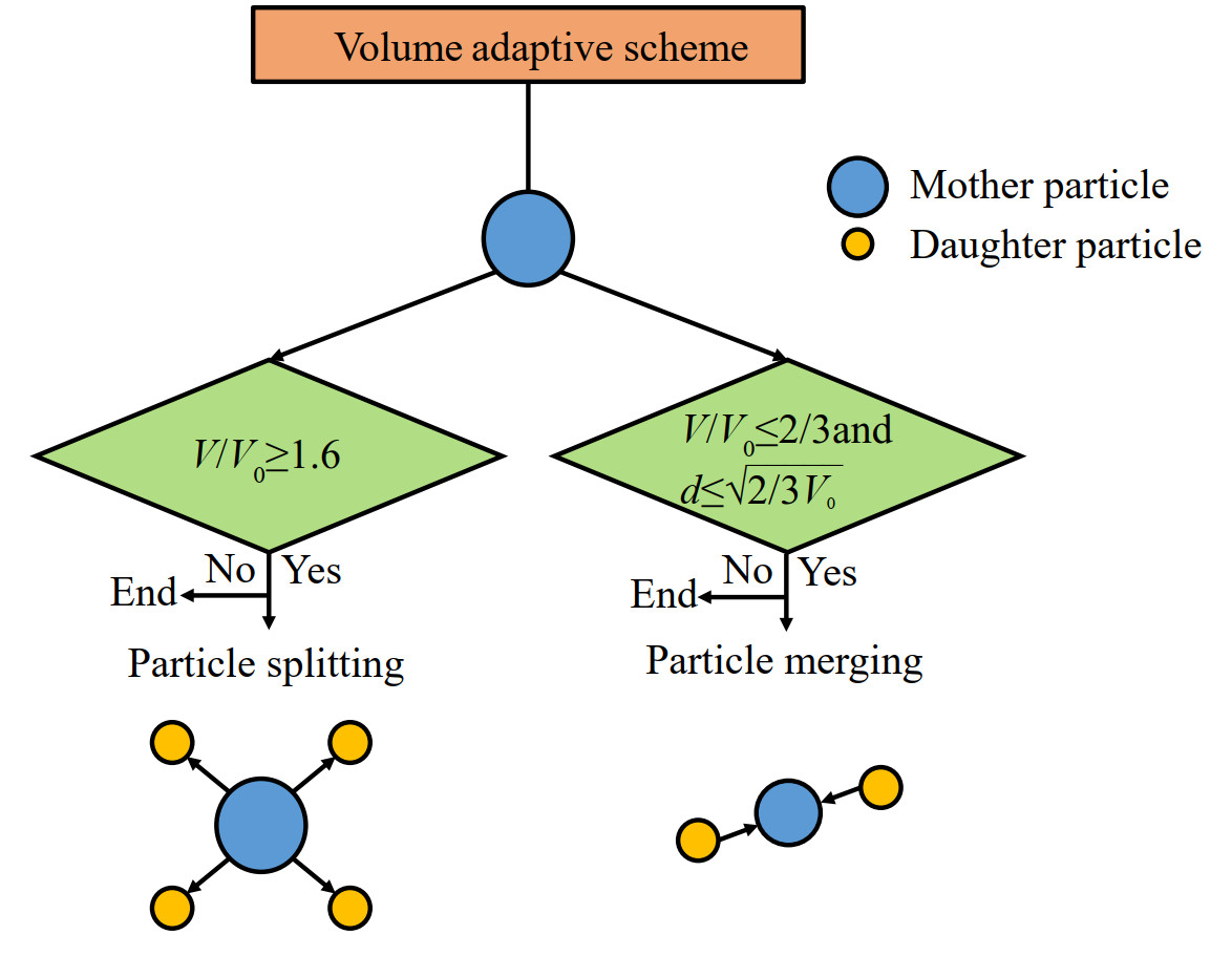Figure  2  Sketch showing the volume adaptive scheme where V₀ represents the initial particle volume and d is the distance between two pairwise particles (Sun et al., 2021)

Download: Full-Size Img

where V_max=1.6 V₀ is obtained from Eq.(14). Accordingly, after splitting, the minimum particle volume of daughter particles is 0.4 V₀, and the maximum volume variation for all particles remains less than 0.6V₀. Other field quantities of the daughter particles can be obtained via the following criteria (Sun et al., 2021) as

where the subscript d and m denote the daughter particles and mother particles, respectively.

As shown in Figure 2, the particle merging is triggered with two conditions i.e. particle volume and distances. When the distance d between two pairwise particles satisfies $d\le \sqrt{(2/3){{V}_{0}}}$ which means the two merging particles are neighbors, and their volumes decrease to V_min (restriction on shrinkage of particle volume), the two particles would be merged into one particle with volume 2V_min. Similar to particle splitting (Sun et al., 2021), the volume variation between before and after merging should also satisfy the relation as follows:

Solving Eq. (16), V_min=2/3V₀ is obtained. The quantities of the merged particle (Sun et al., 2021) are assigned by following equations:

where the two daughter particles are denoted with the subscript d and superscripts 1 and 2, while the merging particle is denoted with the subscript m.

In the present axisymmetric SPH scheme, (see Eqs. (15) and (17)), since the fluid is assumed to be weakly-compressible, the smoothing lengths of all particles remain constant during the simulations, which helps to avoid the update of smoothing length and hence improves the computational efficiency.

In addition, in Sun et al. (2021b), the VAS is applied in the rising rubble problem, while in the present work, we co-opt and implement it to the water entry problems and correspondingly, the interaction between solid and fluid is supposed to be considered. Therefore, according to Newton's second law, the motion of moving rigid bodies in the vertical direction is obtained as follows

where M is the mass of moving bodies and the force F^z is calculated according to the balance between fluid particles (i) and ghost particles (j), see more details in the following section. Rotation is not considered in this work.

2.6   Boundary conditions

In the present work, the solid wall boundaries are discretized into ghost particles. The boundary-setting of water entry problems is plotted in Figure 3, taking the case of the water entry of the cone with β =20° as an example. The free-slip solid boundary is enforced on the solid wall. This is enforced by ignoring the viscous force between fluid and ghost particles. Following Adami et al. (2012), the pressure of ghost particle p_g is extrapolated from the neighboring fluid particles to prevent boundary penetration. The formula is written as

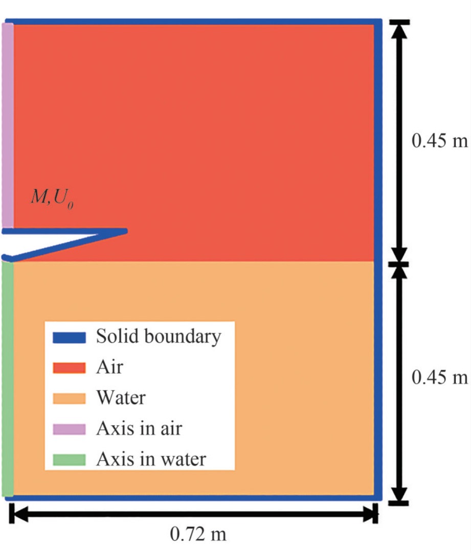Figure  3  Sketch for the numerical set up of the SPH simulations of the axisymmetric water entry problem (take the cone with deadrise angle of β=20° as an example)

Download: Full-Size Img

where the subscripts g and f denote the ghost particles and fluid particles, respectively. In addition, a sponge layer is implemented inside the stationary solid boundary to prevent pressure wave reflection. More details can be referred to Sun et al. (2015).

As for the treatment of multi-phases interface, an interface sharpness force F_i^s is introduced to the momentum equation to maintain the sharpness of the gas-water interface, see more details in Grenier et al. (2009). The compressibility of the air phase can be negligible when simulating the slamming stage of water entry problems (Yang and Qiu, 2012; Wang and Soares, 2020). But the air phase is supposed to be considered in the latter water entry process after the closing of the cavity, (see e.g. Wang and Soares (2020); Lyu et al. (2021)). But in the present work, we only focus on the slamming stage, so the air compressibility is not considered.

2.7   Computational cost

Implementing the axisymmetric SPH scheme, the 3D water entry problem can be simulated in two dimensions, which reduces the particle number and saves the computational cost effectively. Therefore, most simulations are finished in one day using 8 cores parallel computing on a desktop computer with Inter(R) Core(TM) i9-11900K CPU. However, for the cases with the highest particle resolution, R/Δx= 400 in this work, the time step becomes very small, the particle number reaches 4.5 million and therefore it takes several days to finish the SPH simulation. Even so, the particle number used in the axisymmetric SPH model is much reduced, which allows for the using of refined particle resolutions to capture the local pressure peak. In contrast, in purely 3D SPH simulations the computational costs would be much higher and capturing the local flow details is relatively difficult since the particle number in 3D would increase by several orders of magnitude.

3   Numerical results and discussions

3.1   Description of the axisymmetric water entry problem

In the current work, to extend the applicability of the axisymmetric SPH model to 3D axisymmetric water entry problems, following the experiment by De Backer et al. (2009), water entries of a rigid sphere and two rigid cones with deadrise angles of 20° and 45° are selected. The parameters of mass and touch down velocity are listed in Table 1. Schematic diagrams of the sphere and cones are shown in Figure 4. The local pressure is probed at two locations signed as P₁ and P₂, represented by the coefficient C_P (Nair and Bhattacharyya, 2018), defined as:

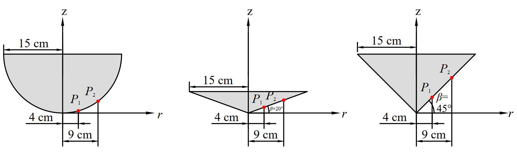Figure  4  The sketch of the water entry bodies. Sphere (left) and cone with β = 20° (middle) and β = 45° (right) (De Backer et al., 2009). The length of body along the radial written as R=0.15 m

Download: Full-Size Img

where P₀ and U₀ are the background pressure and touchdown velocity, respectively.

3.2   Convergence analysis

In this section, a convergence analysis is performed based on the comparison of the pressure coefficients between SPH results of different particle resolutions as well as the experimental data (De Backer et al., 2009). For sphere water entry, four particle resolutions i. e. R/Δx= 50, R/Δx= 100, R/Δx= 200 and R/Δx= 400 are adopted. The pressure coefficients C_P monitored at P₁ with four particle resolutions are plotted in Figure 5. In the initial particle distribution, the bottom of the sphere and water surface are apart as one particle spacing, i.e. Δx. That is to say, larger Δx means a little bit longer touch down distance so that a longer time is needed to reach the pressure peak. As plotted in Figure 5, with a finer particle resolution, the instant of pressure peak is closer to the one of experiment data (De Backer et al., 2009). With a rough particle resolution, the local high pressure peak is not resolved. At the finest particle resolution R/Δx= 400, the value of peak pressure is closest to the experimental data.

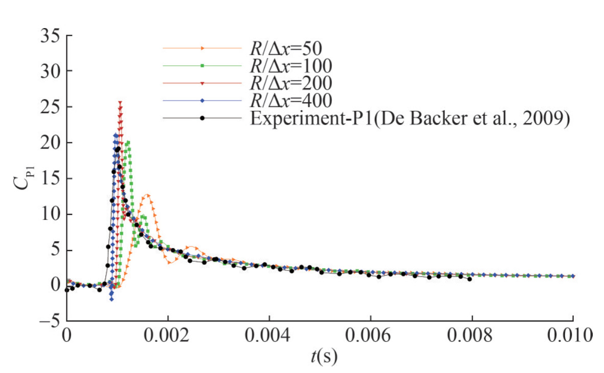Figure  5  Time evolution of the impact pressure probed at location P₁ of sphere with four particle resolutions: SPH results are compared with experimental data (De Backer et al., 2009)

Download: Full-Size Img

To discuss the oscillating of the value of peak impact pressure at R/Δx= 200, the local pressure fields with particle resolutions R/Δx= 200 and R/Δx= 400 are compared in Figure 6. As one can observe, at the lower particle resolution R/Δx= 200, the pressure field near the probing location P₁ encounters oscillations while with the refined one, i.e. R/Δx =400, the pressure field becomes much smoother and shows less noise. The comparison implies that the uncertainty of peak pressure is tightly related to the particle resolution. The local oscillation of the pressure could lead to the changing of peak pressure since in SPH, the local pressure is measured on a single particle, while not the pressure averaged on the probe panel with an area larger than several particles. Comprehensive discussions on the uncertainty analysis of numerical simulations of slamming problems can be referred to Wang et al. (2021).

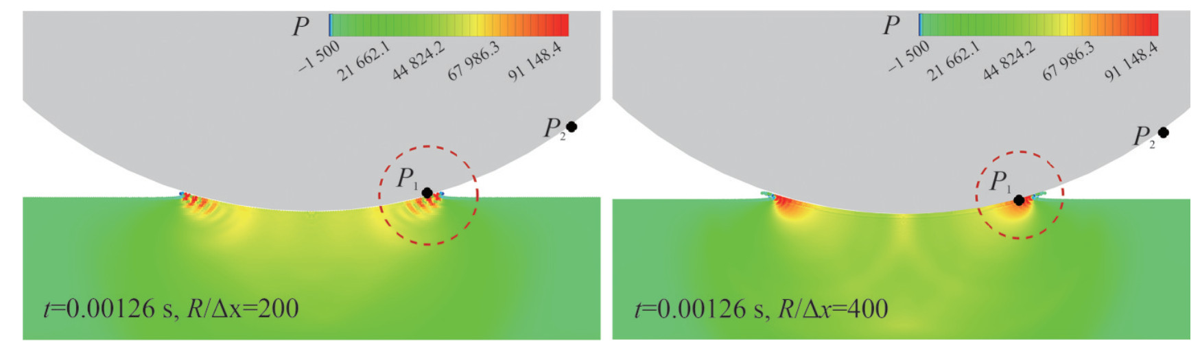Figure  6  The pressure field when peak pressure propagates to the probing location P₁ for the sphere water entry simulated with particle resolutions R/Δx = 200 (left) and R/Δx = 400 (right)

Download: Full-Size Img

Thanks to the reduction of one dimension, the particle number used in axisymmetric SPH is less than that in 3D SPH simulations and therefore it is easier to refine particles to obtain better pressure field. In addition, in fully 3D SPH simulations, doubling the particle resolution will bring a particle number of eight times more, while with the present axisymmetric SPH scheme, doubling the particle resolution only increases the particle number to four times, which is much more efficient.

Based on the discussion above, the convergence study of the cases of two cones is directly simulate with particle spacing R/Δx= 200 and R/Δx= 400. As shown in Figure 7, time evolutions of the impact pressure are quite similar, indicating that for the cases of the cone's water entry, the particle resolutions R/Δx= 200 and R/Δx= 400 can be both applicable. Comparing the impact pressure of the sphere and cones, due to the smaller deadrise angle at the bottom of the sphere, the pressure peak is higher and sharper so that a higher particle resolution is needed. From above discussions, the water entry problem of the sphere is discussed in the following sections with the finest particle resolution R/Δx= 400 while for the cases with cones, the particle resolution R/Δx= 200 is used.

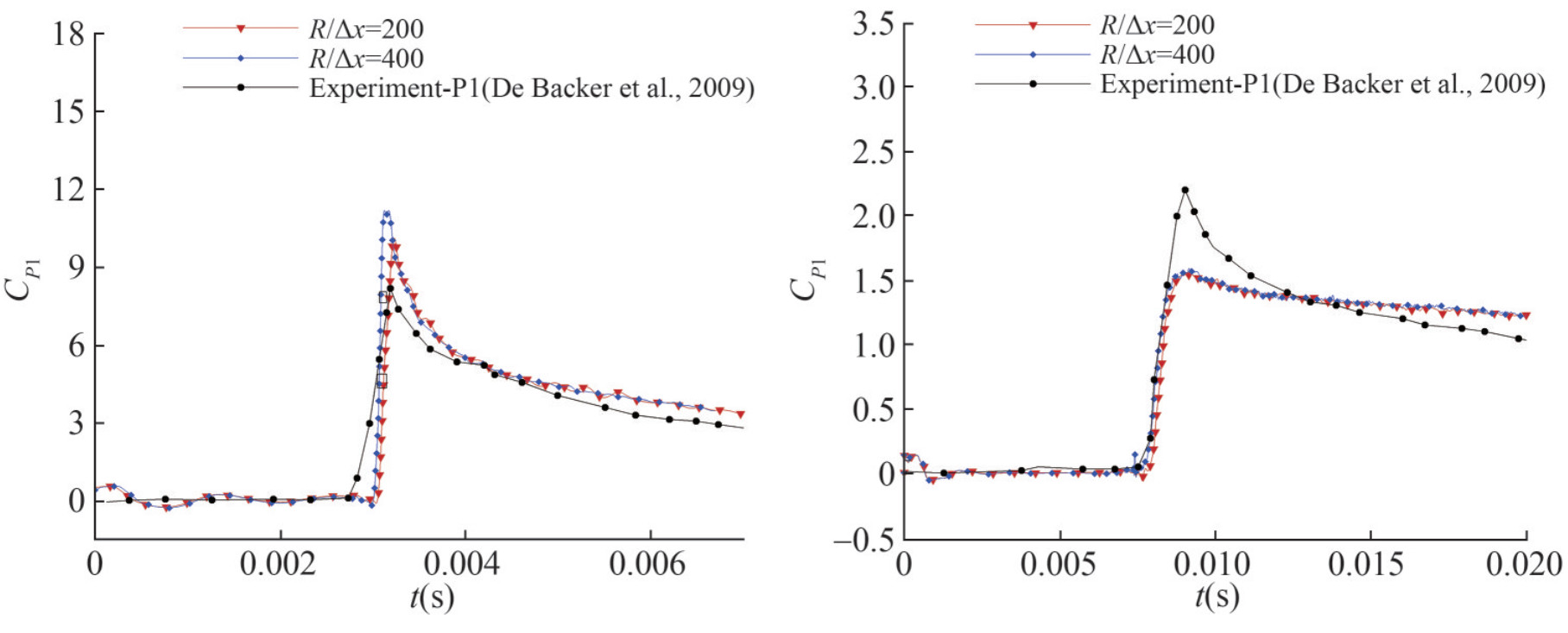Figure  7  Time evolution of the impact pressure probed at location P₁ of cones with deadrise angle 20° (left) and 45° (right) with R/Δx = 200 and R/Δx = 400: SPH results are compared with experimental data (De Backer et al., 2009)

Download: Full-Size Img

3.3   Water entry of a sphere

The water entry of a sphere is simulated, validated and discussed in this part. The mass of the sphere is M=11.5 kg and touchdown velocity is U₀=4.0 m/s as stated above.

The time histories of the impact pressure probed at two different locations (P₁ and P₂) are also plotted in Figure 8 where the SPH result is compared with experimental data (De Backer et al., 2009) and other numerical results obtained via FVM (Nair and Bhattacharyya, 2018). As one can see, the tendency of the pressure evolutions agrees well between the numerical results and the experiment data (De Backer et al., 2009), but a little discrepancy for the pressure peaks is also observed. Generally, the numerical monitors are more sensitive to transient variation of pressure comparing with the experimental sensors. This is because, in experiments, pressure is measured by averaging pressure over the area of the sensor panel while in the SPH simulations, pressure can be captured on a single particle which is much smaller than the sensor panel, which can, therefore, cause a higher pressure peak for the cases of smaller deadrise angle, i.e. the water entries of sphere and cone with smaller deadrise angle, e.g. β= 20°. A similar analysis was also conducted by Wang et al. (2015). Observing the result at location P₂, the SPH result has a better agreement with the FVM result (Nair and Bhattacharyya, 2018) including the rising time and peak values. In addition, to further validate the accuracy of the SPH results, the vertical motion of the sphere, including the impact velocity and penetration depth, is compared with reference results, see Figure 9. The impact velocity is similar to the experimental data (De Backer et al., 2009) and numerical result (Nair and Bhattacharyya, 2018). Moreover, with time gone by, the SPH result is closer to the experimental data compared to the FVM result. Probing the penetration depth, a good agreement is achieved between SPH results and both reference results.

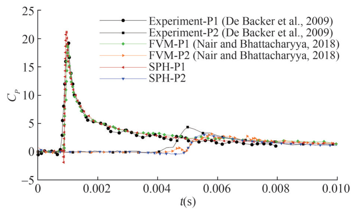Figure  8  Pressure probed at two locations P₁ and P₂: SPH results compared with experimental data (De Backer et al., 2009) and FVM results (Nair and Bhattacharyya, 2018)

Download: Full-Size Img

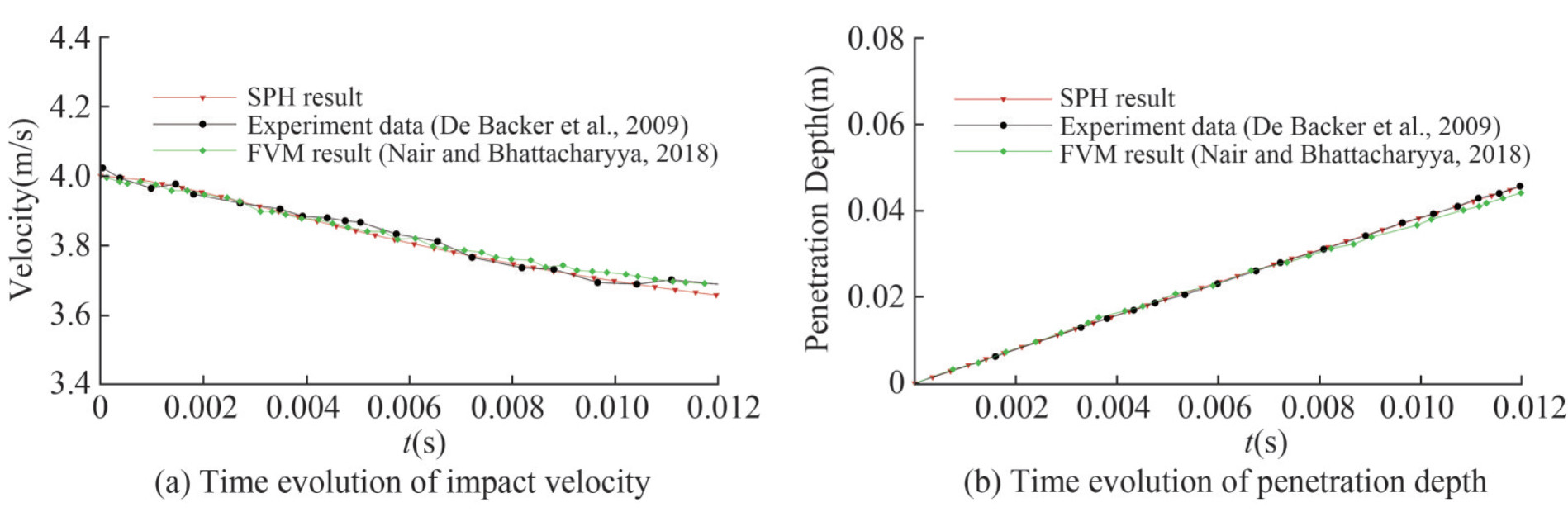Figure  9  Vertical motion of water entry of sphere: SPH results compared with experimental data (De Backer et al., 2009) and FVM results (Nair and Bhattacharyya, 2018)

Download: Full-Size Img

The snapshots during the water entry process are displayed in Figure 10. We note that the air particles are blanked to better visualize the water surface and splashing jets. It can be observed that the qualitative comparison between the experiment (De Backer et al., 2009) and SPH also shows good agreement. Further, the splashing of water jets can be accurately captured. In general, the axisymmetric SPH results are fairly satisfactory.

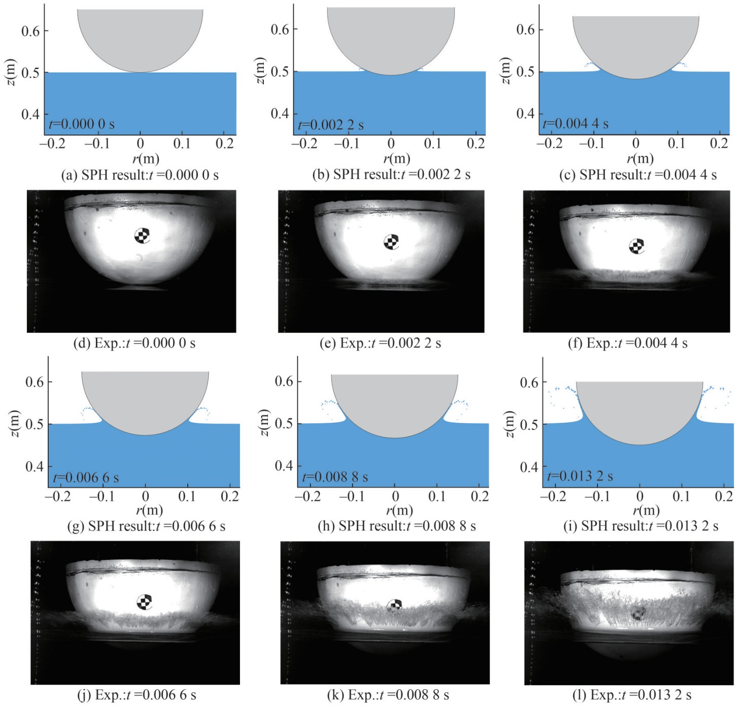Figure  10  Comparison between the present axisymmetric SPH results and the experimental snapshots in De Backer et al. (2009) for the water entry of a sphere

Download: Full-Size Img

Figure 11 displays the pressure field around the sphere at different time instants. It is demonstrated that the present axisymmetric SPH model is able to provide a smooth pressure field, which is very important for estimating the slamming loads in ocean engineering.

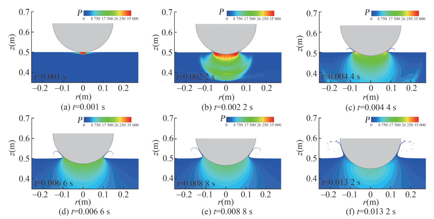Figure  11  The pressure fields at several time instants for the water entry problem of sphere

Download: Full-Size Img

3.4   Water entry of a cone with β = 20°

In this part, the water entry problem of a cone with deadrise angle of 20° is simulated and discussed. Figure 12 shows the time evolutions of the impact pressure measured at locations P₁ and P₂. The comparison is made between SPH simulations, experimental data (De Backer et al., 2009) and FVM results (Nair and Bhattacharyya, 2018). As one can observe, the numerical result of C_P probed in P₂ agrees well with the reference solution. At P₁, the trend of the pressure coefficient of three methods resembles each other, while the pressure peak value of SPH result is a little larger than the other two. However, C_P probed at P₁ after the peak and the C_P probed at P₂ are both closer to experiment data compared with the FVM results. The discrepancy of pressure peak at P₁ can be caused by the uncertainty of the pressure probe when measuring the slamming pressure at a small deadrise angle near the bottom of the cone. As shown in Wang et al. (2015), repeated experiments show a large deviation (error bars) at the instant of peak pressure. Further, the weakly-compressible assumption (the pressure is linked to the density linearly) in the present SPH scheme may also lead to the difference of the numerical results.

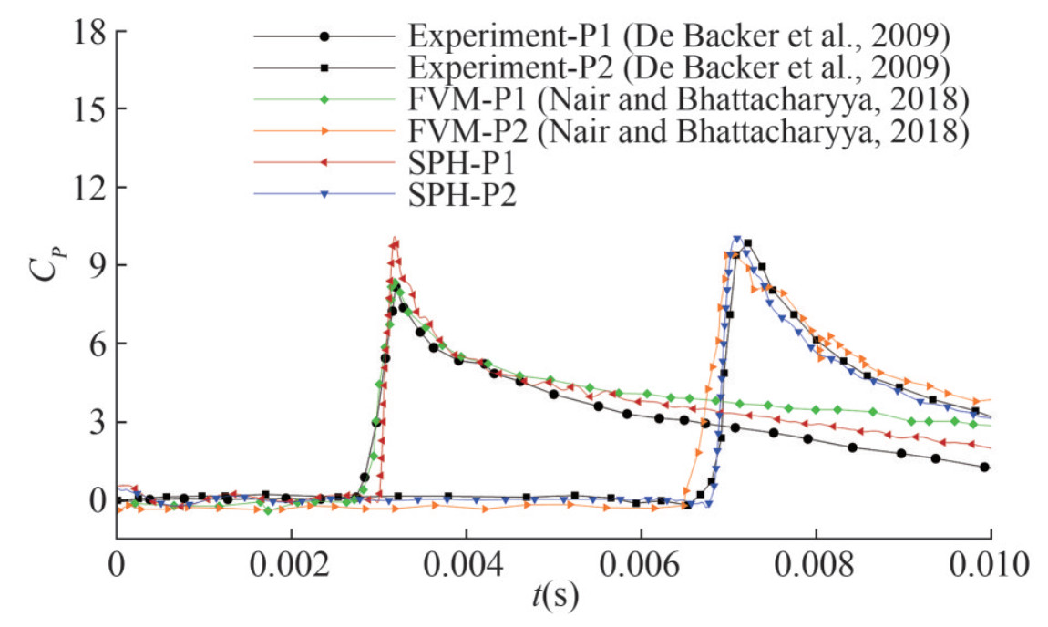Figure  12  Pressure probed at two locations P₁ and P₂ of cone with deadrise angle of β=20°, compared with experimental data in De Backer et al. (2009) and results of Nair and Bhattacharyya (2018) using FVM, respectively

Download: Full-Size Img

Figure 13 shows the vertical velocity and penetration depth compared with reference results. As it is plotted, the penetration depth shows good agreement with experimental data and FVM results. As for the velocity, the SPH result shows good agreement with only slight difference appearing at the latter stage. Figure 14 shows the comparison of the snapshots between SPH and experiment (De Backer et al., 2009). Observing the free surface deformation, the water splashing can be well captured in SPH, which could be challenging for grid-based methods. Therefore, it is demonstrated that the axisymmetric SPH model is able to accurately simulate the water entry problem of a cone with a small deadrise angle of 20°. Figure 15 depicts the pressure field around the cone. As one can see, a smooth pressure field is obtained again and the maximum pressure is located near the intersections between the cone surface and the free-surface.

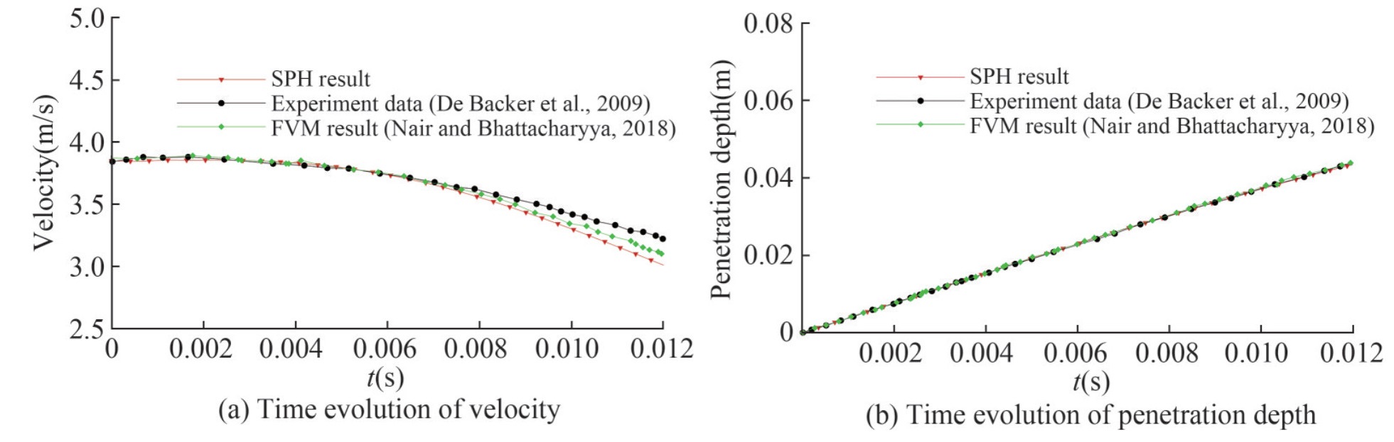Figure  13  Vertical motion of water entry of the cone with deadrise angle β=20°

Download: Full-Size Img

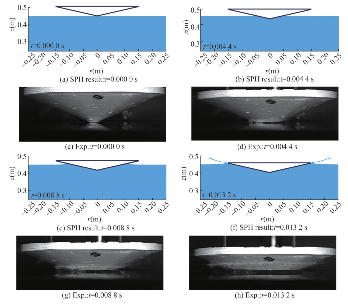Figure  14  Results of the water entry problem of a cone with deadrise angle of β=20°. Comparison between the present axisymmetric SPH results and the experimental snapshots in De Backer et al. (2009)

Download: Full-Size Img

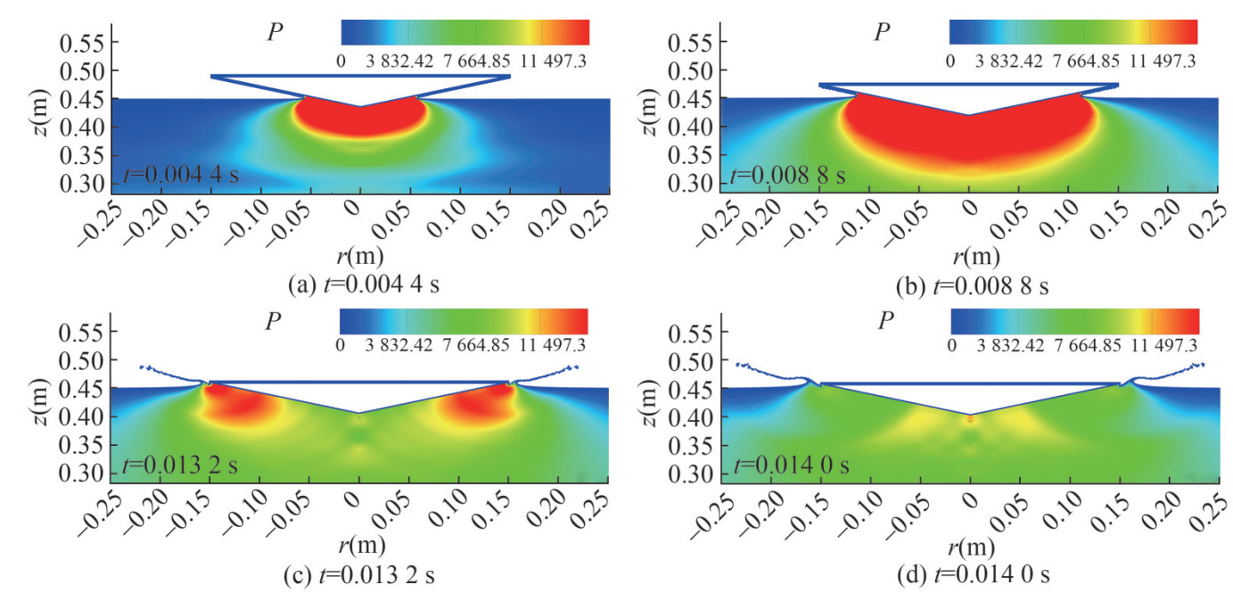Figure  15  The pressure fields at several time instants for the water entry problem of the cone with β=20°

Download: Full-Size Img

3.5   Water entry of a cone with β = 45°

In this part, a cone with deadrise angle of 45° entering undisturbed water is simulated. The time evolution of impact pressure monitored at the two locations P₁ and P₂ is shown in Figure 16. The time instant of pressure rise is accurately predicted by both SPH and FVM solvers (Nair and Bhattacharyya, 2018), while lower pressure peak is predicted at location P₁ and a larger pressure peak is predicted at P₂. As discussed by Iafrati et al. (2015), the local pressure measured in experiments is very sensitive and can be affected by many uncertainties, which is related to the probes and their installation. As also discussed by Wang et al. (2015), by repeating the same water entry experiment, the error bar of the peak pressure was not negligible. There are many uncertainties that could affect the exact peak value of pressure. Therefore, for cone with deadrise angle of β =45°, the reason why the pressure peak at P1 is underestimated is still an open problem. However, at P₂, the SPH result is obviously closer to the experimental data. In addition, comparing the peak values of C_P between cases with deadrise angles of 20° and 45°, the C_P of β = 20° is significantly larger than the one of β = 45°, confirming that the deadrise angle plays an important role in the slamming load. It can also be observed qualitatively that, for the case with a larger deadrise angle of β =45°, the lasting time of the high pressure is longer and the pressure variation is slower than the simulation for the cone with deadrise angle of β =20°. The comparison of the cone's vertical motion is shown in Figure 17. An accurate match is presented in the initial stage while the difference starts to appear after the first pressure peak. This result is also reported in Nair and Bhattacharyya (2018) and Wang and Soares (2014). Different to the velocity curves, the penetration depth can be accurately predicted and a good agreement is obtained between SPH and reference results.

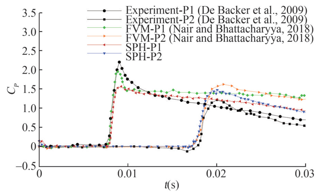Figure  16  Pressure probed at two locations P₁ and P₂ of cone with deadrise angle of β =45°, compared with experimental data in De Backer et al. (2009) and results of Nair and Bhattacharyya (2018) using FVM respectively

Download: Full-Size Img

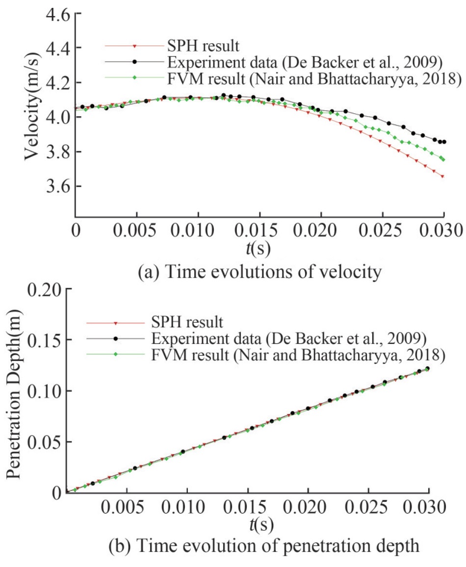Figure  17  Vertical motion of water entry of the cone with deadrise angle β=45°

Download: Full-Size Img

Figure 18 shows the comparison between the SPH and experimental snapshots (De Backer et al., 2009). Obviously, the qualitative comparison presents a good agreement. Further, the pressure field can be well predicted without noise, as shown in Figure 19.

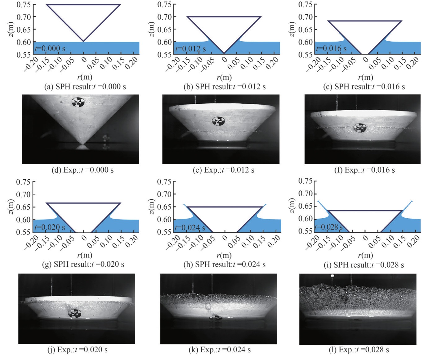Figure  18  Results of the water entry problem of a cone with deadrise angle of β=45°. Comparison between the axisymmetric SPH results and the experimental snapshots in De Backer et al. (2009)

Download: Full-Size Img

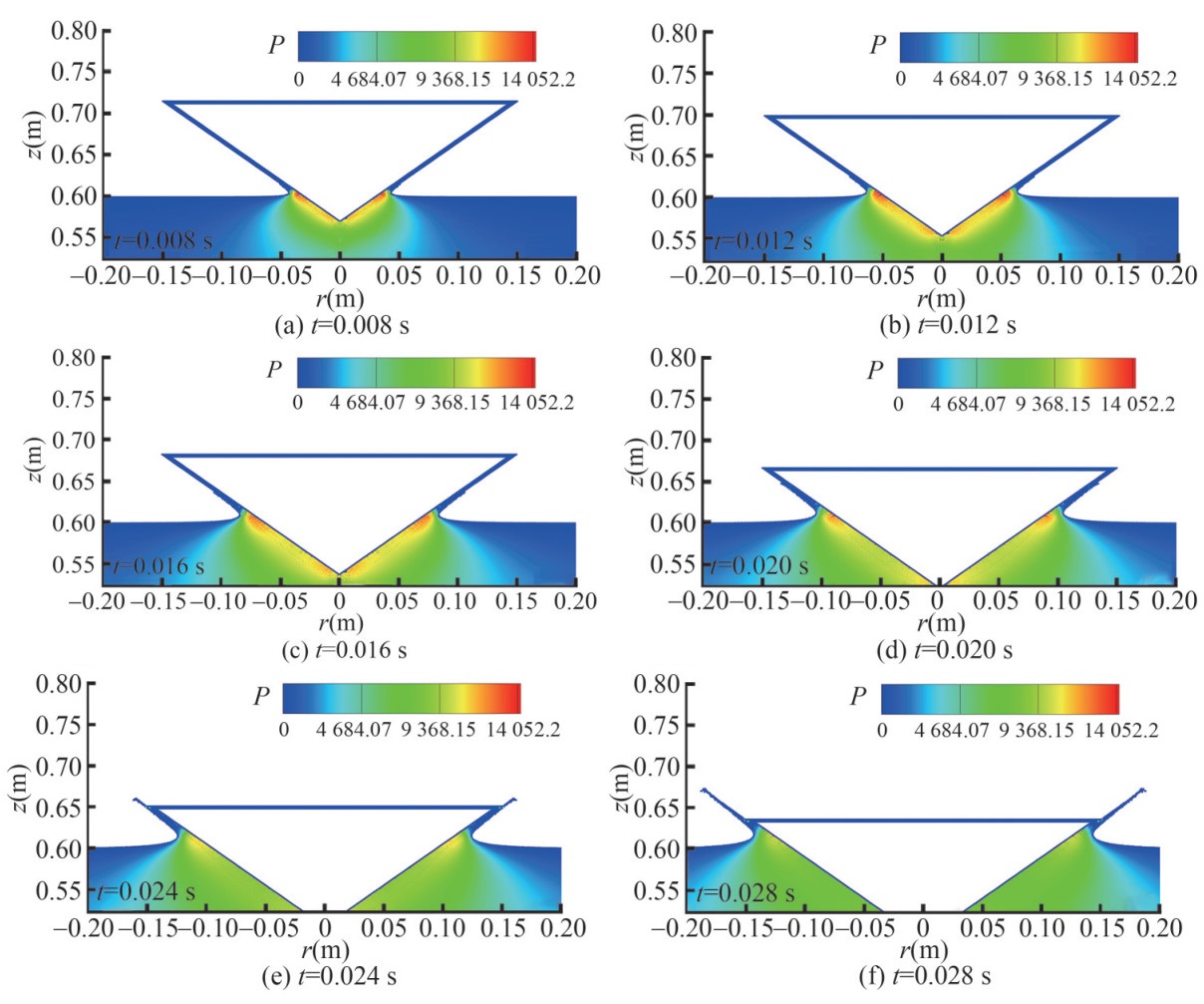Figure  19  The pressure fields at several time instants for the water entry problem of the cone with β=45°

Download: Full-Size Img

4   Conclusions and perspectives

In this work, an axisymmetric SPH model is applied to solve different axisymmetric water entry problems, including water entry of spheres and cones with different deadrise angles. Based on the comparisons between SPH results and experimental data, the axisymmetric SPH model is shown to be accurate, reliable and efficient for such kind of water entry problems. The local impact pressure of a moving body with a small deadrise is predicted well with refined particle resolutions, which is challenging in terms of the computational cost for fully three dimensional SPH simulations, while the axisymmetric SPH model can sufficiently improve computational efficiency and achieves high numerical accuracy. In addition, the splashing jets are successfully captured with the two-phase SPH scheme and agree fairly well with the experimental snapshots.

In future studies, the present axisymmetric SPH model will be further extended for solving water entry problems with higher speeds, studying the impact pressure considering the fluid compressibility effects. The compression of the gas cavity entrapped during water entry should be considered to study the water entry dynamics after pinch-off (see e. g. the 2D study in Lyu et al. (2021)). In addition, the present axisymmetric SPH scheme is limited to the water entry problems of axisymmetric bodies. The 3D SPH simulation for water entry of marine structures with complex shapes is also necessary to be developed and the numerical efficiency can be improved with the implementation of Adaptive Particle Refinement (APR) (Chiron et al., 2018) and GPU parallel computing (Lyu et al., 2022b).