1   Introduction

Path planning is one of the core technologies in autonomous underwater vehicles (AUVs), and it is also a key link in realizing autonomous navigation and operation (Sun et al. 2020). Path planning in underwater robots refers to finding a collision-free path from the initial state to the target state according to certain evaluation criteria in the water environment containing obstacles. In addition, to a certain extent, path planning technology marks the intelligence level of underwater robots (Gasparetto et al. 2015; Sariff and Buniyamin 2006). However, compared with other types of mobile robots, the working environment of underwater robots is a large-scale three-dimensional (3D) space. The complexity of the underwater environment increases the difficulty of path planning. At the same time, the robot's position, energy consumption, self-attitude, and motion constraints should be considered (Gu et al. 2005). Therefore, it is very important to choose a reasonable and suitable path planning method for underwater robots.

Path planning methods for underwater robots can be divided into two categories: traditional approaches and intelligent approaches. Traditional approaches include path planning methods based on the road map construction method (Lozano-Pérez 1990), element decomposition method (Li 2012; Tanakitkorn et al. 2014), A* algorithm, D* algorithm, and artificial potential field (APF) method. The A* algorithm, D* algorithm, and APF method are the most widely used path planning approaches at present. The A* algorithm is suitable for static path planning (Hart et al. 1972). D* algorithm is a dynamic A* algorithm, which is suitable for solving the dynamic path planning problem by detecting the change in the previous node or nearby nodes of the shortest path (Carsten et al. 2006). The APF method is a virtual method proposed by Khatib etc. (Khatib 2003; Volpe and Khosla 1990). The intelligent path planning approaches include swarm intelligence-based methods and the method based on machine learning (Sun et al. 2020). Path planning methods for underwater robots based on swarm intelligence mainly include genetic algorithm (Xu and Li 2010; Xu and Yao 2008), ant colony algorithm (Liu et al. 2016; Wang et al. 2008), and firefly algorithm (Dong 2013; Liu et al. 2015). Algorithms based on swarm intelligence are relatively mature in global path planning, but they do not have a high real-time performance. Concerning the application of machine learning to the path planning for underwater robots, Zhu et al. focused on the situation of sudden obstacles, using environmental changes to cause changes in neuron excitation and activity output values, and thereby outputting collision-free path points (Zhu et al. 2015). To sum it up, traditional path planning methods are simple to describe and easy to implement. However, they generally lack flexibility and the ability to be applied in 3D complex underwater environments. Intelligent methods make up for many shortcomings of traditional methods. They can solve global and local path planning problems. However, based on the basic environment model, they can obtain high real-time planning.

Considering the above-listed drawbacks of the two common approaches, in this paper, the RRT algorithm is adopted as the basic algorithm to study for the path planning of underwater robots. The RRT algorithm is chosen for three main reasons. First, the RRT algorithm is based on a tree structure and random sampling. Therefore, rather than an arbitrary geometric curve between two points, the route from the point to be extended and the new point could be generated by the kinematics and dynamics simulations of robots. Thus, it is suitable for solving dynamic path planning problems. Second, based on random sampling, the RRT algorithm does not need to search all points in the space and model the obstacle space accurately. Lastly, RRT algorithms have advantages in multidimensional spaces. The higher the dimensionality is, the more the node states are. For traditional path planning methods, these algorithms can easily cause dimensionality disasters. However, RRT algorithms are based on random sampling. In a high-dimensional space, they just need more dimensions for sampling, rather than sampling every state in the space.

The search randomness of RRT algorithms makes them have a strong exploration ability. However, it will lead to blindness while planning a certain path. At present, to solve this problem, scholars have proposed some strategies. In the early stage, a single RRT-tree was mainly used for searching. To improve the search speed, scholars proposed biased RRT (Lavalle and Kuffner 2000) and bidirectional RRT (Jr and Lavalle 2000) search algorithms. Therefore, improved RRT algorithms generally include two categories, namely, heuristic algorithms and bidirectional search approaches, which improve the convergence speed to a certain extent. To consider kinematic constraints of the intelligent vehicles, Liu, et al. proposed a target-biasing strategy, which reduces the nodes of trees and improves the search efficiency and running time of an algorithm (Liu et al. 2017). Wang proposed a smooth splicing algorithm (Wang 2014). By optimizing the connection line between random points, the path is generated under the constraint of the motion system. However, the above-mentioned improved RRT algorithms can only plan a relatively optimal path at the cost of search efficiency, which would increase the complexity and searching time of path planning. Therefore, how to plan an optimized path without influencing the running efficiency of RRT algorithms is the problem. Recently, combined algorithms have performed well in solving this problem. By combining membrane computing, genetic algorithm, and the APF method, hybrid approaches successfully reduce time complexity (Orozco-Rosas et al. 2019b) and speed up the computation (Orozco-Rosas et al. 2019a). Inspired by the advantages of hybrid approaches, APF, a goal-oriented algorithm, may be a good choice for improving the performance of RRT algorithms.

Inspired by the two problems, the contributions of this study lie in the following aspects. First, the RRT algorithm is combined with the concepts of AAF in the APF method to guide random trees to grow in the direction of the target point. Based on the common AAF-RRT algorithm with a constant attractive force, an improved AAF-RRT algorithm with a proportional attractive force is proposed to enhance the goal orientation of the algorithm and reduce the computation resource. Second, other researchers mainly focus on studying obstacle avoidance on the global path, which has been planned for AUVs (Cai et al. 2020). To simultaneously plan an optimal and global path, in this study, a two-layer path planner with path smoothing is designed, which combines the global planning based on the proposed AAF-RRT algorithm and the approaches of the local planning. Third, based on the simulation results, the proposed improved AAF-RRT algorithm is verified to perform better than the common AAF-RRT algorithm in the three aspects, namely, search ability, collision-avoidance ability, and the ability to pass through narrow passages. Accordingly, based on the proposed AAF-RRT, the two-layer path planner can successfully plan the global and optimal path for AUVs when adding sudden obstacles to a simulated map.

2   Preliminaries for the RRT and APF

In this section, the concepts, characteristics, and planning process of the RRT algorithm and APF approach will be illustrated in detail.

2.1   RRT algorithm

Uninterruptedly searching the state space of robots via random sampling is the basic principle of RRT algorithms. It can be generally divided into two steps. First, a random tree is rapidly established. Then, an effective path from the initial point to the goal point is queried based on the random tree. The corresponding pseudocode of RRT is shown in Algorithm 1.

The detailed steps of algorithm 1 can be illustrated in the following steps:

Step 1 Initialize the whole statespace. Define the initial point x_init, the number of samples K, and the step size t between the two points.

Step 2 Use the function Random_State () to randomly generate a point x_rand.

Step 3 Use the function Nearest_Neighbor () to find the point x_near closest to the point x_rand.

Step 4 Get the extension vector using the function Selet_Input () and get the new point x_new with the step size t and extension vector u.

Step 5 Determine whether there is an obstacle from x_near to x_new. If it does not exist, then add the point x_new to the tree vertex and connect x_new with x_near.

Figure 1 vividly shows the growth of a random tree in a simulated environment. The blue triangle and red triangle represent the start point and goal point, respectively. Green circles denote points in the tree, and the blank circle denotes the sampling point. Located in the center of the figure, the two white irregular frustums of a pyramid represent the two obstacles in the environment. The expanding process of RRT can be illustrated as follows. After sampling point 5 in the map, the RRT algorithm would figure out the nearest point 3 in the tree. Then, the new point 4 would be added in the tree connected with point 3 at a prescribed step size.

Figure  1  Growth process of random trees in RRT

Download: Full-Size Img

2.2   APF approach

The APF method is a classical path planning algorithm for robots. The APF regards the target position and obstacles as objects that have attractive and repulsive forces on robots, respectively. Therefore, the APF contains two kinds of force fields: AAF formed by the target position and artificial repulsive field (ARF) formed by various obstacles. The robot would move along the synthetic force of the attractive force and repulsive forces. This synthetic force is given as follows:

where x denotes the coordinate position of the intelligent vehicle in the environment, F_att(x) is the attractive force that guides the vehicle to move to the goal position, and F_rep(x) is the repulsive force that makes the vehicle avoid obstacles. F (x) is the synthetic force of F_att(x) and F_rep(x).

Figure 2 shows the force analysis of an intelligent vehicle in the APF algorithm. The blue oval denotes an intelligent vehicle in a simulated environment. The red triangle and white frustum of a pyramid still represent the goal point and obstacle in the environment, respectively. According to the previous illustration of the APF, F₁ and F₂ are the repulsive forces that two obstacles give to the intelligent vehicle. F₀ is the attractive force given from the goal position to the position of the intelligent vehicle. After the synthesis of the three forces, F₃ is the final force that the vehicle receives. The vehicle would move under the guidance of F₃.

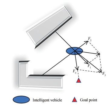Figure  2  Force analysis of an intelligent vehicle in the APF

Download: Full-Size Img

3   Improved AAF-RRT algorithm

As the randomness of RRT causes its search blindness, to improve the search efficiency, we add the concepts of the AAF in APF to the extension of random trees in the RRT algorithms. Then, the goal point in the search environment would have an attractive field for robots. Considering that there exist the judging criteria for the collisions among points and obstacles in RRT, the concept of ARF in the APF approach is not necessary to be added to RRT algorithms. After this combination, RRT becomes goal-oriented, and this improved RRT algorithm is named AAF-RRT algorithm in this paper, which is a kind of RRT algorithm integrated with AAF.

In the concept of AAF, the potential function carries the information of targets, which should be delayed to RRT. Then, the random tree can move in the direction of the potential field from the targets when exploring the space. In addition, the excellent exploration ability of RRT can make up for the shortcoming that the potential field method easily falls into a local minimum. After all, we combine RRT and AAF by adding the idea of target attraction into the extension of the RRT random tree. The detailed illustration of the extension in AAF-RRT is as follows: First, after randomly generating the n^th sample point p_rand(n), the corresponding n^th nearest point, p_near(n), is obtained. Then, for the n^th nearest point p_near(n), R(n) represents the extension vector that the random point p_rand(n) gives to p_near(n). The attractive vector A(n) is given from the goal point to p_near(n). R(n) and A(n) simultaneously affect the extension of the random tree. Therefore, the random tree can grow toward the target point with a certain and rational trend.

According to the basic RRT algorithm, the extension vector of the nearest point p_near(n) can be expressed in the following mathematical formula:

where R(n) denotes the extension vector that the n^th random point p_rand(n) gives to the n^th nearest point p_near(n). ε represents the step size in the RRT algorithm. Moreover, the fraction $\frac{p_{\text {rand }}(n)-p_{\text {near }}(n)}{\left\|p_{\text {rand }}(n)-p_{\text {near }}(n)\right\|}$ denotes the unit vector of the line connecting p_rand(n) and p_near(n), which later would become the unit vector of R(n).

Referring to Eq. (2), the artificial attractive vector A(n) of the AAF-RRT algorithm constructed in this work can be elaborated by Eq. (3).

where ρ(n) is the attractive factor, which can change the target bias of the random tree. A(n) is the attractive vector given to the n^th nearest point p_near(n) from the goal point p_goal. ε still represents the step size of the algorithm. $\frac{p_{\mathrm{goal}}-p_{\mathrm{near}}(\mathrm{n})}{\left\|p_{\mathrm{goal}}-p_{\mathrm{near}}(\mathrm{n})\right\|}$ denotes the unit vector of the line connecting p_goal and p_near(n). Therefore, the final guided extension vector F(n) is as follows:

Then, the calculation equation for the new extended point p_new(n) can be obtained by Eq. (5).

Eq. (5) shows that the calculation for p_new(n) includes two parts, i.e., the extension vector from the sample point p_rand(n) and the attractive vector from the goal point p_goal. Then, based on Algorithm 1 of the basic RRT algorithms, the pseudocode of the AAF-RRT algorithms is shown in Algorithm 2.

Compared with Algorithm 1, v and the function Attractive_Input () are added to the algorithm. v denotes the attractive vector given from the target point. After getting the coordinate positions of the goal point and the nearest point, the function Attractive_Input () could calculate the attractive vector. Then, during the formation of the new point, the nearest point would synthesize two vectors, i. e., extension vector u and attractive vector v, to get the new point. In terms of connecting the nearest point x_near and new point x_new, the direction of this connection line is determined by the synthetic vectors of u and v. Moreover, the corresponding formation and extension of the random tree are shown in Figure 3.

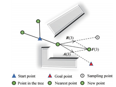Figure  3  Extension of the random tree in AAF-RRT algorithms

Download: Full-Size Img

Patterns in Figure 3 are generally the same as those in Figure 1. The difference between the two figures only lies in the formation of the new point. Figure 3 takes the tree extension in point 3 as an example. R(3) is the extension vector given by the sampling point 5. A(3) is the attractive vector from the goal point. F(3) is the final guided extension vector synthesized by R(3) and A(3). Then, under the influence of F(3), the new point 4 is successfully formed and added into the random tree. In the previously designed AAF-RRT algorithm, the expression of ρ(n) in Eq. (3) is not determined yet. ρ(n) is described as the attractive factor that the n^th point to be extended receives from the AAF of the goal point. For the current common AAF-RRT algorithm, the attractive factor is set to be constant. However, if all the points in the random tree receive the same attractive factor, then the point closer to the target point will receive the same gravitational force as the rest of the points. This condition may cause the point to jitter near the target point when the tree is extended near the target point, which would affect the convergence of the planning algorithm. Therefore, an improved AAF-RRT algorithm is proposed. In this algorithm, ρ(n) is proportional to the Euler distance between the goal point and the n^th point to be extended. As for the first assumption that the attractive factor for the points to be extended is unchanged and constant, Eq. (6) is chosen to describe the attractive factor in the common AAF-RRT algorithm.

where ρ(n) denotes the attractive factor for the n^th point to be extended and k₁ denotes the unchanged and constant value of attractive factors in this kind of situation. Unlike the common AAF-RRT algorithm presented above, for the improved AAF-RRT algorithm, the attractive factor is set to be proportional to the Euler distance between the n^th point to be extended and the goal point.

The corresponding attractive factor ρ(n) can be expressed as follows:

where k₂ denotes the coefficient given to the attractive factor ρ(n). p_goal and p_near(n) represent the coordinate positions of the goal point and n^th point to be extended, respectively. ‖p_goal-p_near(n)‖ denotes the Euler distance between the mentioned two points. Here, when the point to be extended is closer to the goal point, the attractive force it receives would become smaller. This phenomenon would be helpful for the convergence of paths to be planned.

Based on the work done in Liu et al. (2017); Song et al. (2010); Wang et al. (2020), compared to the basic RRT algorithm, the common AAF-RRT algorithm with a constant attractive force could accelerate the convergence of the path and shorten the path length. Therefore, to make the comparison of the simulation results comprehensive and convincing, in Section 6, we present the simulations conducted among three algorithms, namely, basic RRT algorithm, common AAF-RRT algorithm with constant attractive forces, and improved AAF-RRT algorithm with a proportional attractive force.

4   Two-layer path planner

The proposed two-layer path planner is divided into two parts: First, the global path would be planned by the chosen path planning algorithm. Then, the position of the sudden obstacle in the environmental model would decide whether the path should be replanned.

4.1   Two steps for the path planner

The diagram of the proposed path planner is shown in Figure 4, which describes the specific steps of how to conduct the planning process combining global planning and local planning. The first step is global planning, which gets the global path by the specific path planning algorithm. The other steps in the diagram all belong to the local planning. The detailed illustration of the local planning is as follows: After a sudden obstacle is added to the environmental model, the planner would identify its position and determine whether it conflicts with the previous path. Then, according to the determination, the planner would replan the path or not.

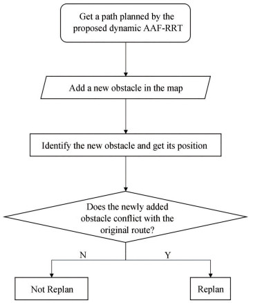Figure  4  Diagram of the two-layer path planner

Download: Full-Size Img

4.2   Path smoothing

Owing to the randomness of the RRT algorithm, the algorithm has a strong exploration ability. However, the randomness will lead to the blindness of path planning. Accordingly, the planned path would have more redundant points, which increases the corners and the length of the path. Therefore, many optimization methods have been used to determine sub-optimal and optimal paths. The most common and simplest optimization method is pruning, which aims to cut out unnecessary nodes. As shown in Figure 5, if there is no collision between point 1 and point 3, then the line from point 1 to point 2 and the line from point 2 to point 3 can be directly replaced with the line from point 1 to point 3.

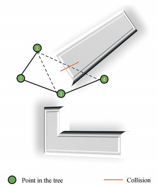Figure  5  Diagram of the two-layer path planner

Download: Full-Size Img

After path smoothing is conducted by pruning, redundant points could be correspondingly cut, and the planned path would be shorter according to the triangle inequality.

5   Simulation results

Simulations are conducted in two parts: The first part is the simulations for comparing the improved AAF-RRT algorithm with the common AAF-RRT algorithm and basic RRT algorithm. The simulation includes the selection of the environmental mazes, outputting the figures on the views of the random trees, processing time and path length obtained by the algorithms, and conducting the rank-sum tests on the data samples. The second simulations are executed for the two-player path planner. A new environmental maze is chosen for the simulation. Then, the figures on the planned path after the path smoothing and path replanning after the emergence of the sudden obstacles are outputted.

5.1   Simulations for the algorithms

Several mazes are used for studying RRT algorithms. From a comprehensive view, three different mazes with different layouts of obstacles are chosen as the simulation environments, as shown in Figure 6. Based on the simulation results under the three simulation environments, the searching ability of the three algorithms, i. e., basic RRT algorithm, common AAF-RRT algorithm, and improved AAF-RRT algorithm, can be deeply compared and analyzed.

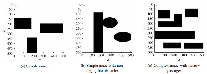Figure  6  Three different mazes with three different layouts

Download: Full-Size Img

In the figure, the black pattern represents the obstacle that intelligent agents cannot pass, whereas the white areas are where the agents can pass. The coordinate system of the maze is established as follows: The upper long side of the maze is the x-axis. The right side is the positive direction of the x-axis. The left side of the maze is the y-axis, the positive direction of which is the downward direction. The green hollow circles in the mazes are the initial points, and the red hollow circles are the goal points. The corresponding coordinate positions of the two types of points are unified to be (10, 10) and (290, 290), respectively. Figure 6(a) shows a simple maze with three square obstacles. There is no obvious obstacle blocking the agents from the start point to the goal point. This simple maze is used for the preliminary exploration of the search speed, search performance, and collision-avoidance ability of the three algorithms. For further exploration of the collision-avoidance ability, another simple maze, shown in Figure 6(b), contains the non-negligible obstacles on the line from the start point to the goal point. Considering the poor ability of the basic RRT algorithm to pass through the narrow passage in the environment, a complex maze with the narrow passage is selected. Whether AAF-RRT algorithms can improve this kind of ability would be answered and confirmed.

Before the simulation of the three algorithms under the three different mazes, we unified several standards for the subsequent simulations. First, the coordinate positions of the start point and goal point are set as (10, 10) and (290, 290), respectively. The maximum iterations of the simulations are 10 000. Two indexes are chosen to reflect the searching ability and collision-avoidance ability of the three planning algorithms, which are the processing time (s) reflecting the search speed and the path length reflecting the search performance. The overview of the random tree and final planned path would be outputted under the three algorithms, which could directly reflect the search randomness of the sampling-based planning algorithms. Lastly, according to Eqs. (5) and (6), we assume that k₁ and k₂ in the subsequent simulations are equal to 0.02 and 0.0001, respectively.

5.1.1   Simple maze

For the preliminary exploration, simulations are conducted in the simple maze. Again, the black areas represent the obstacles in the maze, and white areas represent the passable areas in the maze. The simulation results are shown in Figure 7.

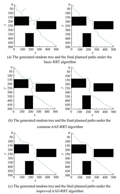Figure  7  Whole view of the generated random trees and final planned paths in the simple maze under the three algorithms

Download: Full-Size Img

The left sides of Figure 7 show the simulation results of the basic RRT. The middle and right sides show the results of the AAF-RRT algorithms with constant attractive and proportional attractive forces, respectively. Figure 7(a) shows the whole view of the three generated random trees, where the nodes in the tree become less from left to right. This result indicates that AAF-RRT algorithms can reduce the search randomness of the basic RRT and improve the running efficiency of the algorithms. Conversely, the improved AAF-RRT algorithm with proportional attractive forces behaves better in this kind of utility compared with the common AAF-RRT algorithm. In terms of the final planned paths shown in Figure 7(b), there exists no obvious difference among the three planned paths. However, due to the improvement in the randomness of the RRT algorithms, the planned paths are smooth in the AAF-RRT algorithms.

After conducting the same simulation ten times, the data samples of the processing time and path length under the three algorithms are outputted, which are shown in Figures 8 and 9, respectively. Based on the data shown in the figures, the samples are all non-normal. Therefore, the rank-sum test should be used to preliminarily determine whether the gap between two data samples is evident. With the significance level set to 0.05, the rank-sum test results on the processing time and path length among the three samples are also shown in Figures 8 and 9, where "*" indicates that the overall difference between the two data samples is significant.

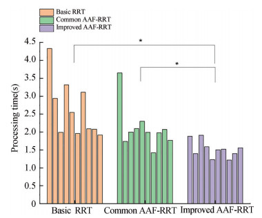Figure  8  Processing time and rank-sum test results of the three algorithms on the simple maze

Download: Full-Size Img

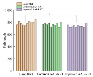Figure  9  Path length and rank-sum test results of the three algorithms on the simple maze

Download: Full-Size Img

Two conclusions can be derived from the simulation results. First, in terms of the processing time, the gap between the common AAF-RRT and basic RRT is not significant, whereas the gap between the improved AAF-RRT and basic RRT and the gap between the improved AAF-RRT and common AAF-RRT are all significant. For the path length, only the gap between the improved AAF-RRT and basic RRT is significant. Then, a further conclusion can be obtained. The improved AAF-RRT behaves the best among the three algorithms in terms of processing time. Common AAF-RRT cannot behave better than the basic RRT in the processing time. Moreover, AAF-RRT behaves better than the basic RRT in the path length, whereas common AAF-RRT still does not have a significant difference with the basic RRT.

To sum it up, through the preliminary exploration of the simple maze, the simulation results confirm that the two AAF-RRT algorithms can improve the search randomness of the RRT algorithm. They can also improve the running efficiency and search performance of the basic RRT algorithm. Furthermore, the improved AAF-RRT behaves the best in terms of the running efficiency and search performance among the three algorithms.

5.1.2   Simple maze with obstacles on the line

Based on the former simulations, the simulation environment is upgraded from a simple maze to a simple maze with obvious obstacles on the line. This line refers to the virtual line from the initial point to the goal point in the environment. The aim of this simulation is mainly to determine whether AAF-RRT algorithms could improve the collision-avoidance ability of basic RRT algorithms. Similar to the former simulations, figures on the whole view of the random trees and the final planned paths are successfully outputted, as shown in Figure 10.

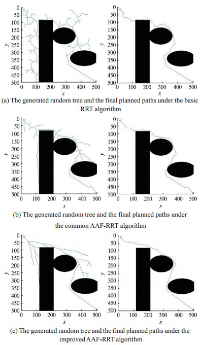Figure  10  Whole view of the generated random trees and final planned paths in the simple maze with obstacles on the line under the three algorithms

Download: Full-Size Img

Compared with those in Figure 7, the meanings of the patterns stay unchanged in Figure 10. The numbers of nodes in the random trees still turn less from top to bottom in Figure 10. Moreover, the trees tend to be smooth under the AAF-RRT algorithms. Therefore, with the upgrading of the maze, the AAF-RRT algorithms still behave better than the basic RRT algorithm. In terms of the emergence of the obvious obstacles on the line from the initial point to the goal point, the simulation results also show that the AAF-RRT algorithms have a better collision-avoidance ability without the loss of running efficiency. Running efficiency is reflected by the nodes in the random tree.

The corresponding simulation data of the three algorithms are shown in Figures 11 and 12, where the rank-sum test results are also shown. The differences among the three algorithms are all significant. Therefore, based on the overlook of the data samples, the order of the planning performance from good to bad is as follows: improved AAF-RRT algorithm→common AAF-RRT algorithm→basic RRT algorithm.

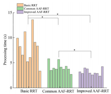Figure  11  Processing time and rank-sum test results of the three algorithms on the simple maze with obstacles on the line

Download: Full-Size Img

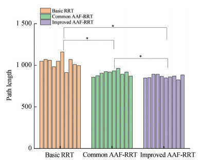Figure  12  Path length and rank-sum test results of the three algorithms on the simple maze with obstacles on the line

Download: Full-Size Img

Based on the simulation results in the second maze, the AAF-RRT algorithms can improve the collision-avoidance ability of the RRT algorithms without the loss of the running efficiency and searching ability. At the same time, based on the common AAF-RRT algorithm, the improved AAF-RRT algorithm can further improve the search speed and reduce the path length.

5.1.3   Complex maze with narrow passages

The former two simulation results under the two simple mazes have verified that the AAF-RRT algorithms improve the search randomness and searching ability of the basic RRT algorithms. Considering the poor ability of the RRT algorithms in passing through the narrow passage, a complex maze with a narrow passage is chosen as the simulation environment. This maze contains a narrow passage around the target point. It also includes obstacles on the line from the initial point to the target point. The simulation results of the random trees and planned paths are shown in Figure 11.

Figure 13(a) shows that the random tree under the basic RRT algorithm is very complicated and almost covers the entire maze. During the conducted simulation process under the basic RRT algorithm, the random tree extends in an extremely slow manner when passing the narrow passages. However, from the other two whole views of the random trees under the two AAF-RRT algorithms, the nodes of the random trees are significantly reduced, especially in the improved AAF-RRT algorithm with a proportional attractive force. Comparing the two random trees under the two AAF-RRT algorithms, the tendency of the random trees toward the goal point is more obvious under the improved AAF-RRT algorithm. This comparison indicates that the improved AAF-RRT algorithm behaves better in terms of the ability to pass the narrow passage than the common AAF-RRT algorithm.

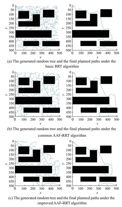Figure  13  Whole view of the generated random trees and final path in the complex maze with the narrow passage under the three algorithms

Download: Full-Size Img

The simulation results under the three algorithms are shown in Figures 14 and 15. Based on the positions of the "*, " in the searching speed, the order of the performance from good to bad is as follows: improved AAF-RRT algorithm→ common AAF-RRT algorithm→ basic RRT algorithm. However, in the path length tests, only the difference between the improved AAF-RRT algorithm and the basic RRT algorithm is significant.

Figure  14  Processing time and rank-sum test results of the three algorithms on the simple maze with obstacles on the line

Download: Full-Size Img

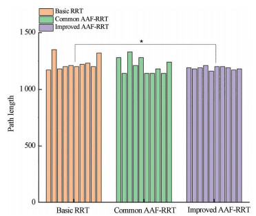Figure  15  Processing time and rank-sum test results of the three algorithmson the simple maze with obstacles on the line

Download: Full-Size Img

Based on the above analysis of the simulation results, compared with the common AAF-RRT algorithm, the improved AAF-RRT algorithm can effectively improve the ability to pass the narrow passage of the RRT algorithms better. This kind of improvement has not been found and verified by other researchers.

5.1.4   Local minima trap

One of the challenges in the APF approach is the local minima trap, which may happen when the two APFs, i.e., AAF and ARF, cancel each other out. For example, when an obstacle is located between the robot and target position, a local minima trap may happen. Although the gradient of these local minima points is zero, they are not the target point set in the environment. Moreover, this kind of local minima trap exists in other path planning methods, such as genetic algorithms (Gong and Peng 2002), clustering algorithms (Dash et al 2003; Xu and Franti 2004), and deep learning methods (Kawaguchi 2016).

In our proposed AAF-RRT algorithms, a local minima trap also exists in some situations. The existence of the local minima trap in APF approaches directly caused the emergence of that in the AAF-RRT algorithms. The emergence of the local minima trap also indicates that the combination of APF and RRT has advantages and disadvantages. Thus, we should highlight its strengths and avoid its weakness as much as possible. Many ways can be done to solve the local minima trap. One method is to introduce a high-level planner, which would make the robot not only use the detection information from the sensors at any time but also maintain the ability of global planning (Dong 2009). Some remedial solutions allow the robot to fall into the local optimum and then use other solutions to fix the problem. For example, a disturbance or backtracking could be added to the local minima trap to jump out of the local minima points (Morris 1993).

Considering that the objective of this study is to explore the search utilization of the improved AAF-RRT algorithm, an easy and simple solution is chosen to escape the local minima trap for the AAF-RRT algorithms. The solution is to manually reduce the relevant attractive factors until the path can get into the goal point. In the two AAF-RRT algorithms proposed in this paper, the relevant attractive factors are k₁ and k₂ in Eqs. (5) and (6). During the previous numerical simulations under the three RRT algorithms, when adopting the k₁ and k₂ of the simulations in the former two simple mazes, the local minima trap emerges in the complex maze under the two AAF-RRT algorithms with k₁ = 0.2 and k₂ = 0.002, respectively. By using the proposed solution of reducing the two attractive factors, the local minima trap can be effectively escaped when k₁ = 0.02 and k₂ = 0.000 1. The four overviews of the random tree of the emergence and escape of the local minima trap in the mentioned situation are shown in Figures 16 and 17. Figure 16 shows the situation under the common AAF-RRT algorithm, whereas Figure 17 shows the situation under the improved AAF-RRT algorithm. As shown in the two figures, although the attractive factors are manually adjusted and reduced, the proposed solution to escape the local minima trap for the AAF-RRT algorithms is useful and feasible.

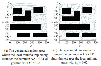Figure  16  Whole view of the generated random trees where the local minima trap emerges be overcomed under the common AAF-RRT algorithm

Download: Full-Size Img

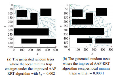Figure  17  Whole view of the generated random trees where the local minima trap emerges and be overcomed under the improved AAF-RRT algorithm

Download: Full-Size Img

5.2   Simulations for the two-layer path planner

A new simulation environment is configured for the two-layer path planner, which is shown in Figure 16. As shown in Figure 18, the blue and green squares denote the initial node and goal node, respectively. The coordinate position of the initial node is set to (2, 2), whereas that of the goal node is set to (49, 24). The black frame in the figure represents the boundary of the environment. The gray patterns denote the obstacles in the environment, which consist of four circular obstacles and four rectangular obstacles.

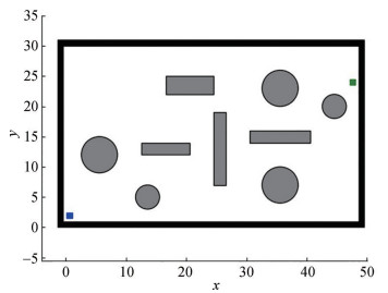Figure  18  Environmental configuration of the simulations for the two-player path planner

Download: Full-Size Img

5.2.1   Two-layer path planner combined with path smoothing

The improved AAF-RRT is chosen to be the planning algorithm in the two-layer path planner. The simulation process of the two-layer path planner consists of two parts according to the description in Section 4.1. First, the global path would be outputted by the planning algorithm. Second, considering the probability of the sudden obstacles in the environment, the path would be replanned according to the positions of the sudden obstacles.

For the first part, the improved AAF-RRT algorithm would be used to generate a global path. To further shorten the path length, pruning is conducted after generating a path. Then, the planned paths with no pruning and pruning are both outputted, which are shown in Figure 19. The red line denotes the path simulated with no pruning, whereas the blue line represents the path simulated with pruning. Then, the corresponding path length is reduced from 66.95 to 59.36 by adding pruning.

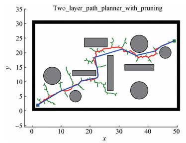Figure  19  Planned paths without pruning and with pruning

Download: Full-Size Img

5.2.2   Two-layer planner added with sudden obstacles

Based on the planned path simulated in Figure 19, we add the sudden obstacles thrice one by one. The fish pattern represents the sudden obstacle. The geometric center of the first obstacle is located in (10, 7), which conflicts with the previously planned path. Therefore, a new path is planned after adding the obstacle, as shown in Figure 20(a). The meanings of the red and blue lines are unchanged. The second obstacle is added at (15, 22). The obstacle would not conflict with the previously planned path. Therefore, there is no need for the path to be replanned. The previously planned path with pruning would be retained in the red line, as shown in Figure 20(b). Lastly, the third sudden obstacle emerges at (23, 16), conflicting with the previously planned path. Then, the replanned paths are outputted based on the newly added three obstacles, which are also shown in Figure 20(c).

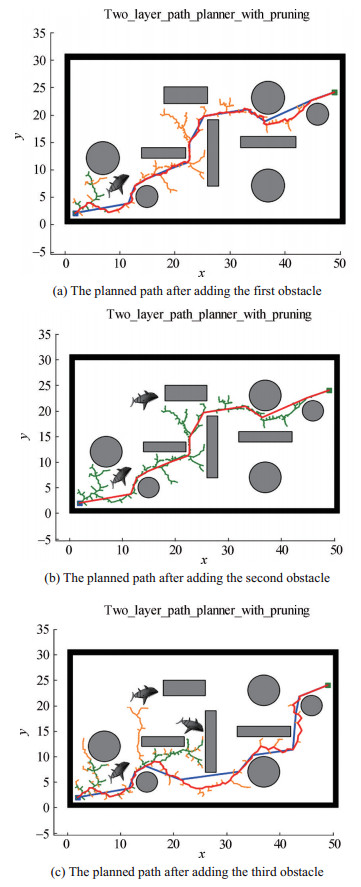Figure  20  Planned paths after the sudden obstacles thrice one by one

Download: Full-Size Img

To sum it up, based on the simulation results, the two-layer path planned can not only search a global path with the help of the improved AAF-RRT algorithm and the pruning process but also effectively replan the path when the sudden obstacle emerges in the environment.

6   Conclusions

In order to improve the search efficiency and collision-avoidance ability of AUVs, this study proposes a specific two-player path planner based on an improved algorithm. By integrating the AAF concept with the RRT algorithm, the proposed AAF-RRT algorithm is verified to perform better than the basic RRT algorithm and common AAF-RRT algorithm. After adding several sudden obstacles to the simulation environment, it is confirmed that the two-layer path planner based on the proposed algorithm can quickly react and effectively avoid obstacles. The two verification results provide a basis for the subsequent practical application of the RRT algorithm in AUVs. They also make stable path planning in harsh underwater environments no longer a luxury.

Thus far, the improved AAF-RRT algorithm and two-layer path planner have only been applied to a two-dimensional environment. In the future, to further explore the feasibility of the algorithm and path planner, a 3D simulation will be conducted. Moreover, it would be interesting to explore whether the expansion direction branches in RRT can refer to the true growth direction of branches in nature.