Gravity Wave Generated by Initial Axisymmetric Disturbance at the Surface of an Ice-covered Ocean with Porous Bed
https://doi.org/10.1007/s11804-021-00241-y
-
Abstract
This paper is concerned with the generation of gravity waves due to prescribed initial axisymmetric disturbances created at the surface of an ice sheet covering the ocean with a porous bottom. The ice cover is modeled as a thin elastic plate, and the bottom porosity is described by a real parameter. Using linear theory, the problem is formulated as an initial value problem for the velocity potential describing the motion. In the mathematical analysis, the Laplace and Hankel transform techniques have been used to obtain the depression of the ice-covered surface in the form of a multiple infinite integral. This integral is evaluated asymptotically by the method of stationary phase twice for a long time and a large distance from the origin. Simple numerical computations are performed to illustrate the effect of the ice-covered surface and bottom porosity on the surface elevation, phase velocity, and group velocity of the surface gravity waves. Mainly the far-field behavior of the progressive waves is observed in two different cases, namely initial depression and an impulse concentrated at the origin. From graphical representations, it is clearly visible that the presence of ice cover and a porous bottom decreases the wave amplitude. Due to the porous bottom, the amplitude of phase velocity decreases, whereas the amplitude of group velocity increases.Article Highlights• This integral is evaluated asymptotically by the method of stationary phase.• The effect of the ice-covered surface and bottom porosity on the surface elevation, phase velocity, and group velocity of the surface gravity waves are analyzed numerically. Also, the significant effect is shown in a number of figures.• The generation of surface gravity waves due to prescribed initial axisymmetric disturbance in the presence of ice cover on a porous sea bed is analyzed here.• Using the Laplace and Hankel transform technique, the depression of the ice-covered surface in the form of multiple infinite integrals is obtained. -
1 Introduction
Ocean wave generation or propagation into or within sea ice fields is a well-established research topic that is currently getting the extensive attention of various researchers. Actually, the sea ice of the polar region bears a significant role in global climate and the conservation of marine life. In the polar region, the seawater freezes due to the very low temperature of the atmosphere. Due to less density of ice than water, ice floats on the ocean's surface so that the ocean is covered by a continuous sheet of ice or broken ice. In recent years the scientific activities in Polar Regions are increasing day by day because, in reality, sea ice covers about 7% of the Earth's surface and about 12% of the world's oceans. There are usually two types of models for floating ice exit. In the first model, the ice is considered to consist of non-interacting floating particles, i.e., broken ice, and in that case, the ocean is said to have an inertial surface (cf, Weitz and Keller 1950; Rhodes-Robinson 1984; Mandal and Mukherjee 1989). In another model, the floating ice is assumed to be in the form of a thin elastic sheet (cf. Fox and Squire 1994; Chung and Fox 2002; Squire 2007; Meylan and Squire 1996 and others). Investigations of such water wave problems have gained reasonable interest due to the effects of internal wave propagation through the marginal ice zone in the arctic regions. Bhattacharjee and Sahoo (2008) analyzed the effect of uniform current on flexural gravity waves generated due to a disturbance such as an initial impulse or an initial depression. Mohapatra and Bora (2009) considered the propagation of oblique waves in a two-layer fluid whose upper layer is bounded above by a thin uniform ice sheet and the lower layer has small bottom undulation. Sturova (2013) derived the velocity potential for a transient source of arbitrary strength in a fluid of infinite depth with an elastic solid cover. The interest behind the study of these problems arises due to their applications in several practice areas, such as large floating plate-like structures, floating airports, etc.
Generally, surface gravity waves are generated due to various kinds of initial disturbances at the surface of an ocean or within the ocean. When a non-spherical shock wave caused by a mid-air blast impinges on the surface of an ocean or some explosion occurs within or above the ocean region, surface waves are generated due to an initial impulsive pressure or initial displacement (elevation or depression). The relevant two-dimensional unsteady motion thus formed was studied in the classical treatises of Lamb (1945) and Stoker (1957), considering the linear theory of water waves. They used the method of Fourier transform and obtained the expression of free surface elevation in the form of infinite integrals, which were then evaluated approximately for large time and distance from the source of the disturbance. These results can be extended in case of any initial surface disturbances across the arbitrary region for uniform finite depth water with a rigid bottom (cf. Wen 1982). Maiti and Mandal (2005) considered the wave generation problem due to initial axisymmetric disturbances on the ice-covered surface of the water. A disturbance is said to be axisymmetric when it is identical in every plane that passes through the axis of a cylinder so that the angular component of the governing equation can be neglected. An axially symmetric disturbance was considered in brief by Kranzer and Keller (1959). They discussed the problem of water waves generated by explosions in the case of three-dimensional unsteady motion in the water of uniform finite depth due to an initial surface impulse or initial surface elevation in a circular area. They also compared their theoretical results with the available experimental results. In the recent past, Banerjea et al. (2011) discussed the wave generation problem due to a line source present in an ice-covered ocean with small bottom undulation. Recently, Das and Mohapatra (2019) considered a particular hydro-elastic model to examine a radiation problem caused by a submerged sphere beneath in an infinitely extended ice-covered sea where the lower surface is enveloped by a flexible base surface. Khuntia and Mohapatra (2020) examined the motion of the fluid in a sea, where the top surface is sealed by a floating ice floe and the bed is of an adaptable type with small distortion. In all of these problems, the authors considered floating ice as a thin elastic plate.
All the aforesaid problems were studied for the ocean with a rigid bottom. In reality, the ocean bottom is composed of porous materials such as rocks, soil, zeolite, biological tissues, etc. However, there is not much work involving the ocean surface covered with a thin ice sheet, and the bottom is composed of some porous materials. So when the water is covered with a thin ice sheet and some porous materials are present at the bottom, the corresponding water wave problems are also of some interest to ocean engineers. There are so many researchers who considered different types of modeling of the problems for the ocean with a porous bottom in the presence of ice-cover. Tsai et al. (2006) studied the problem of wave transformation over a submerged permeable breakwater on a porous slope seabed. They presented several numerical results for the verification of the model and the wave transformation over the submerged breakwater on the porous bottom. Mohapatra (2014) studied the scattering of surface waves by the edge of a small undulation on a porous bed in an ocean with covering thin elastic ice sheet at the upper surface. Paul and De (2014; 2017) considered two types of scattering of plane surface wave problems for the uneven porous bottom, one in a two-layered channel and the other in a three-layered channel. Maiti and Mandal (2014) considered the problem of water wave scattering by a floating elastic plate in an ocean with a porous bed. Gayen and Islam (2018) considered the problem of determining velocity potential due to the presence of a horizontal circular ring in the water of finite depth with a floating elastic plate or a floating membrane at the upper surface and the bottom of the fluid region is composed of the non-dissipative porous medium. Very recently Kundu and Mandal (2019) discussed the generation of surface waves in water with a porous bottom due to various types of prescribed initial axisymmetric disturbances at the free surface. In these problems, the authors consider a special type of porous bottom for which the porosity parameter is taken to be only real and has the dimension inverse of length.
In the present paper, we consider the generation of gravity waves by initial axisymmetric disturbance at the surface of an ice-covered ocean, while the ocean bed is taken to be porous in nature. The problem is formulated as an initial value problem assuming linear theory. Laplace and Hankel transform techniques are used to find the depression of the ice-covered surface in terms of a multiple infinite integral. This multiple integral is approximated by the stationary phase method for two types of initial disturbances namely initial axially symmetric depression or impulse. Finally, the asymptotic form of the ice-covered surface is depicted graphically against a nondimensional distance for a fixed time and against nondimensional time for a fixed distance and different values of nondimensionalized porosity parameter and ice-cover parameters. Also, phase velocity and group velocity of the surface gravity waves are evaluated analytically and numerically. Lastly, appropriate conclusions are drawn for the initial depression of the ice-covered surface and phase velocity, and group velocity of the surface gravity waves.
2 Mathematical Formulation: Formulation of Initial Value Problem
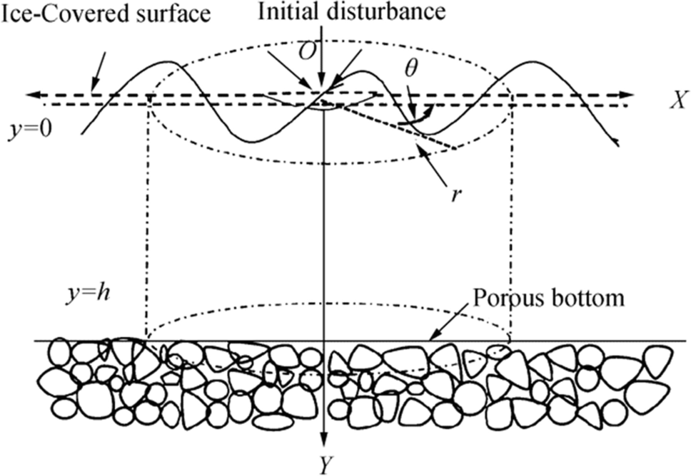
We consider a cylindrical coordinate system $ \left({\boldsymbol{r}}\boldsymbol{ },{\boldsymbol{\theta}},{\boldsymbol{y}}\boldsymbol{ }\right) $ in which the y-axis is taken vertically downwards into the fluid region. The upper surface of the ocean is covered with a thin layer of ice modeled as a very thin elastic sheet having a uniform surface density $ {\boldsymbol{\epsilon}}{\boldsymbol{\rho}} $, where $ {\boldsymbol{\epsilon}} $ is a constant having the dimension of length. Ocean fluid is considered an inviscid, incompressible, and homogeneous liquid of volume density $ {\boldsymbol{\rho}} $. Also, the bottom of the ocean is composed of some specific kind of porous materials which are characterized by a real parameter G having dimension inverse of length. The sketch of the physical model is shown in Figure 1. Wave motion is created due to a sudden initial axisymmetric disturbance at the ice-covered surface.
Since the motion starts from rest, it is irrotational and can be described by a velocity potential $ {\boldsymbol{\phi}}({\boldsymbol{r}},{\boldsymbol{y}},{\boldsymbol{t}}) $, which satisfies Laplace's equation.
$$ \frac{1}{{\boldsymbol{r}}}{\left({\boldsymbol{r}}{{\boldsymbol{\phi}}}_{{\boldsymbol{r}}}\right)}_{{\boldsymbol{r}}}+{{\boldsymbol{\phi}}}_{{\boldsymbol{y}}{\boldsymbol{y}}}=0,{ in the fluid region} $$ (1) Since the bed of the ocean is composed of some porous materials the bottom condition is given by (cf. Maiti and Mandal 2014)
$$ {{\boldsymbol{\phi}}}_{{\boldsymbol{y}}}-{\boldsymbol{G}}{\boldsymbol{\phi}}=0,\boldsymbol{ }{on }{\boldsymbol{y}}={\boldsymbol{h}} $$ (2) where G is the porosity parameter.
The kinematic condition arises due to the assumption of no cavitation between the ice and water. So, the condition gives
$$ {{\boldsymbol{\phi}}}_{{\boldsymbol{y}}}={{\boldsymbol{\eta}}}_{{\boldsymbol{t}}}\boldsymbol{ }{on }{\boldsymbol{y}}=0 $$ (3) where $ {\boldsymbol{\eta}} $ is the depression of the ice cover below its mean position. The linearized dynamic condition at the ice cover is (cf. Chung and Fox 2002)
$$ {\left({\boldsymbol{\phi}}-{\boldsymbol{\epsilon}}{{\boldsymbol{\phi}}}_{{\boldsymbol{y}}}\right)}_{{\boldsymbol{t}}{\boldsymbol{t}}}=\left(1+{\boldsymbol{D}}{\nabla }_{{\boldsymbol{r}}}^{4}\right){\boldsymbol{g}}{{\boldsymbol{\eta}}}_{{\boldsymbol{t}}},\boldsymbol{ }{on }{\boldsymbol{y}}=0 $$ (4) where D is the flexural rigidity of the ice cover and is given by $ {\boldsymbol{D}}=\frac{{\boldsymbol{E}}{{\boldsymbol{h}}}_{0}^{3}}{12\left(1-{{\boldsymbol{\nu}}}^{2}\right){\boldsymbol{\rho}}{\boldsymbol{g}}}, $ E being Young's modulus, $ {{\boldsymbol{h}}}_{0} $ being thickness of the ice sheet and $ {\boldsymbol{\nu}} $ being Poisson's ratio.
The initial conditions at the ice-covered surface are
$$ {\boldsymbol{\phi}}-{\boldsymbol{\epsilon}}{{\boldsymbol{\phi}}}_{{\boldsymbol{y}}}=0,\boldsymbol{ }{on }{\boldsymbol{y}}=0,\boldsymbol{ }{\boldsymbol{t}}=0 $$ (5) $$ {\left({\boldsymbol{\phi}}-{\boldsymbol{\epsilon}}{{\boldsymbol{\phi}}}_{{\boldsymbol{y}}}\right)}_{{\boldsymbol{t}}}=\left(1+{\boldsymbol{D}}{\nabla }_{{\boldsymbol{r}}}^{4}\right){\boldsymbol{g}}{\boldsymbol{\zeta}}\left({\boldsymbol{r}}\right),{on }{\boldsymbol{y}}=0,\boldsymbol{ }{\boldsymbol{t}}=0 $$ (6) when an initial axially symmetric depression $ {\boldsymbol{\zeta}}\left({\boldsymbol{r}}\right) $ of the ice-covered surface at a distance r from the origin is prescribed, and g is the acceleration due to gravity.
Again, when an initial axially symmetric impulse $ {\boldsymbol{F}}({\boldsymbol{r}}) $ is applied per unit area of the ice-covered surface at a distance r from the origin, the initial conditions are
$$ {\boldsymbol{\phi}}-{\boldsymbol{\epsilon}}{{\boldsymbol{\phi}}}_{{\boldsymbol{y}}}=-\frac{{\boldsymbol{F}}\left({\boldsymbol{r}}\right)}{{\boldsymbol{\rho}}},\boldsymbol{ }{on }{\boldsymbol{y}}=0,\boldsymbol{ }{\boldsymbol{t}}=0 $$ (7) $$ {\left({\boldsymbol{\phi}}-{\boldsymbol{\epsilon}}{{\boldsymbol{\phi}}}_{{\boldsymbol{y}}}\right)}_{{\boldsymbol{t}}}=0,{ on }{\boldsymbol{y}}=0,\boldsymbol{ }{\boldsymbol{t}}=0 $$ (8) Introducing a characteristic length l, characteristic time $ \sqrt{\frac{{\boldsymbol{l}}}{{\boldsymbol{g}}}} $ we define the dimensionless quantities as
$$ \begin{array}{l}\overline{{\boldsymbol{r}} }=\frac{{\boldsymbol{r}}}{{\boldsymbol{l}}},\boldsymbol{ }\overline{{\boldsymbol{y}} }=\frac{{\boldsymbol{y}}}{{\boldsymbol{l}}},\boldsymbol{ }\overline{{\boldsymbol{t}} }={\boldsymbol{t}}\sqrt{\frac{{\boldsymbol{g}}}{{\boldsymbol{l}}}},\boldsymbol{ }\overline{{\boldsymbol{\eta}} }=\frac{{\boldsymbol{\eta}}}{{\boldsymbol{l}}},\boldsymbol{ }\overline{{\boldsymbol{h}} }=\frac{{\boldsymbol{h}}}{{\boldsymbol{l}}},\overline{{\boldsymbol{\phi}} }=\frac{{\boldsymbol{\phi}}}{{\boldsymbol{l}}\sqrt{{\boldsymbol{g}}{\boldsymbol{l}}}},\\ \overline{{\boldsymbol{G}} }={\boldsymbol{G}}{\boldsymbol{l}},\boldsymbol{ }\overline{{\boldsymbol{D}} }=\frac{{\boldsymbol{D}}}{{{\boldsymbol{l}}}^{4}},\boldsymbol{ }\overline{{\boldsymbol{\epsilon}} }=\frac{{\boldsymbol{\epsilon}}}{{\boldsymbol{l}}}\end{array} $$ Removing the bars, the dimensionless quantities satisfy
$$ \frac{1}{{\boldsymbol{r}}}{\left({\boldsymbol{r}}{{\boldsymbol{\phi}}}_{{\boldsymbol{r}}}\right)}_{{\boldsymbol{r}}}+{{\boldsymbol{\phi}}}_{{\boldsymbol{y}}{\boldsymbol{y}}}=0 $$ (9) $$ {{\boldsymbol{\phi}}}_{{\boldsymbol{y}}}={{\boldsymbol{\eta}}}_{{\boldsymbol{t}}}\boldsymbol{ }{on}\boldsymbol{ }{\boldsymbol{y}}=0 $$ (10) $$ {\left({\boldsymbol{\phi}}-{\boldsymbol{\epsilon}}{{\boldsymbol{\phi}}}_{{\boldsymbol{y}}}\right)}_{{\boldsymbol{t}}{\boldsymbol{t}}}=\left(1+{\boldsymbol{D}}{\nabla }_{{\boldsymbol{r}}}^{4}\right){{\boldsymbol{\eta}}}_{{\boldsymbol{t}}},\boldsymbol{ }{on }{\boldsymbol{y}}=0 $$ (11) $$ {{\boldsymbol{\phi}}}_{{\boldsymbol{y}}}-{\boldsymbol{G}}{\boldsymbol{\phi}}=0,\boldsymbol{ }{on }{\boldsymbol{y}}={\boldsymbol{h}} $$ (12) The initial conditions at ice-covered surface are
$$ {\boldsymbol{\phi}}-{\boldsymbol{\epsilon}}{{\boldsymbol{\phi}}}_{{\boldsymbol{y}}}=0,\boldsymbol{ }{on }{\boldsymbol{y}}=0,\boldsymbol{ }\boldsymbol{ }{\boldsymbol{t}}=0 $$ (13) $$ {\left({\boldsymbol{\phi}}-{\boldsymbol{\epsilon}}{{\boldsymbol{\phi}}}_{{\boldsymbol{y}}}\right)}_{{\boldsymbol{t}}}=\left(1+{\boldsymbol{D}}{\nabla }_{{\boldsymbol{r}}}^{4}\right){{\boldsymbol{\zeta}}}^{\boldsymbol{^{\prime}}}\left({\boldsymbol{r}}\right),\boldsymbol{ }{at }{\boldsymbol{t}}=0,\boldsymbol{ }\boldsymbol{ }{\boldsymbol{y}}=0 $$ (14) or
$$ {\boldsymbol{\phi}}-{\boldsymbol{\epsilon}}{{\boldsymbol{\phi}}}_{{\boldsymbol{y}}}=-\frac{{{\boldsymbol{F}}}^{\boldsymbol{^{\prime}}}\left({\boldsymbol{r}}\right)}{{\boldsymbol{\rho}}},{ on }{\boldsymbol{y}}=0,\boldsymbol{ }\boldsymbol{ }{\boldsymbol{t}}=0 $$ (15) $$ {\left({\boldsymbol{\phi}}-{\boldsymbol{\epsilon}}{{\boldsymbol{\phi}}}_{{\boldsymbol{y}}}\right)}_{{\boldsymbol{t}}}=0,\boldsymbol{ }{on}\boldsymbol{ }{\boldsymbol{y}}=0,\boldsymbol{ }\boldsymbol{ }{\boldsymbol{t}}=0 $$ (16) as the initial disturbance is axially symmetric depression or impulse at the ice-covered surface and $ {\boldsymbol{\zeta}}\boldsymbol{^{\prime}}({\boldsymbol{r}}) $, $ {\boldsymbol{F}}\boldsymbol{^{\prime}}({\boldsymbol{r}}) $ denote the nondimensional form of initial axially symmetric depression, impulse, respectively.
3 Method of Solution: Laplace and Hankel Transform Techniques
We use Laplace and Hankel transform technique to solve the above initial value problem. Now, let us define Laplace transform of $ \phi \left(r,y,t\right) $ in time $ t $ as
$$ \overline{\phi }\left(r,y,p\right)={\int }_{0}^{\infty }\phi \left(r,y,t\right){{e}}^{-pt}{d}t, p \gt 0 $$ and then define Hankel transform of $ \overline{\phi }\left(r,y,p\right) $ as
$$ \widehat{\overline{\phi }}(k,y,p)={\int }_{0}^{\infty }r\overline{\phi }\left(r,y,p\right){J}_{0}(kr){d}r, k \gt 0. $$ Applying these two transforms to Eqs. (9) to (12) using the conditions (13) to (16) we get the following BVP in $ \widehat{\overline{\phi }} $
$$ {\widehat{\overline{\phi }}}_{yy}-{k}^{2}\widehat{\overline{\phi }}=0 $$ (17) $$ {\widehat{\overline{\phi }}}_{y}=p\widehat{\overline{\eta }}-\widehat{{\zeta }^{^{\prime}}}\left(k\right),{on }y=0 $$ (18) $$ {p}^{2}\widehat{\overline{\phi }}-\left(\epsilon {s}^{2}+1+D{k}^{4}\right){\widehat{\overline{\phi }}}_{y}=\left(1+D{k}^{4}\right)\widehat{{\zeta }^{^{\prime}}}\left(k\right), {on} y=0 $$ (19) or,
$$ {p}^{2}\widehat{\overline{\phi }}-\left(\epsilon {s}^{2}+1+D{k}^{4}\right){\widehat{\overline{\phi }}}_{y}=-\frac{p}{\rho }\widehat{{F}^{^{\prime}}}\left(k\right), {on }y=0 $$ (20) where $ \widehat{{\zeta }^{\boldsymbol{^{\prime}}}}(k) $ and $ \widehat{{B}^{\boldsymbol{^{\prime}}}}(k) $ are the Hankel transforms of $ \widehat{{\zeta }^{^{\prime}}}(k) $ and $ \widehat{{F}^{\boldsymbol{^{\prime}}}}(k) $, respectively.
The bottom condition is
$$ {\widehat{\overline{\phi }}}_{y}-G\widehat{\overline{\phi }}=0, {on }y=h $$ (21) Solution of (17) satisfying (19) and (21) is
$$ \widehat{\overline{\phi }}\left(k,y,s\right)=-\frac{{c}^{2}\widehat{{\zeta }^{^{\prime}}}\left(k\right)}{k\left({p}^{2}+{c}^{2}\right)}\left[\mu \left(k\right){cosh }ky+{sinh} ky\right] $$ (22) where
$$ \mu (k)=\frac{k-G{tanh}kh}{G-k{tanh}kh} $$ (23) and
$$ {c}^{2}=\frac{k(1+Dk^4)}{\epsilon k-\mu (k)} $$ (24) Now, using (18) we get the Laplace–Hankel transform of the depression of the ice-cover in case of initial axially symmetric depression as
$$ {\widehat{\overline{\eta }}}_{D}=-\frac{{c}^{2}\widehat{{\zeta }^{^{\prime}}}\left(k\right)}{p\left({p}^{2}+{c}^{2}\right)} $$ (25) Similarly, in case of initial axially symmetric impulse using Eq. (20) the expression for the depression of the ice-cover is given by
$$ {\widehat{\overline{\eta }}}_{I}=\frac{{c}^{2}\widehat{{F}^{^{\prime}}}\left(k\right)}{\rho (1+D{k}^{4})\left({p}^{2}+{c}^{2}\right)} $$ (26) These expressions of $ \widehat{\overline{\eta }} $ are same as Kundu and Mandal (2019) when $ \epsilon =0, D=0 $ and when $ G=0, h\to \infty $ the expressions are the same as Maiti and Mandal (2005). Equations (25) and (26) can be rewritten as
$$ {\widehat{\overline{\eta }}}_{D/I}=\left\{\begin{array}{c}\widehat{{\zeta }^{^{\prime}}}\left(k\right)\left[\frac{p}{\left({p}^{2}+{c}^{2}\right)}-\frac{1}{p}\right] (initial axially symmetric depression)\\ \frac{\widehat{{F}^{^{\prime}}}\left(k\right)}{\rho (1+D{k}^{4})}\left[\frac{{c}^{2}}{{p}^{2}+{c}^{2}}\right] (initial axially symmetric impulse)\end{array}\right. $$ (27) 3.1 Case A ($ Gh \lt 1 $)
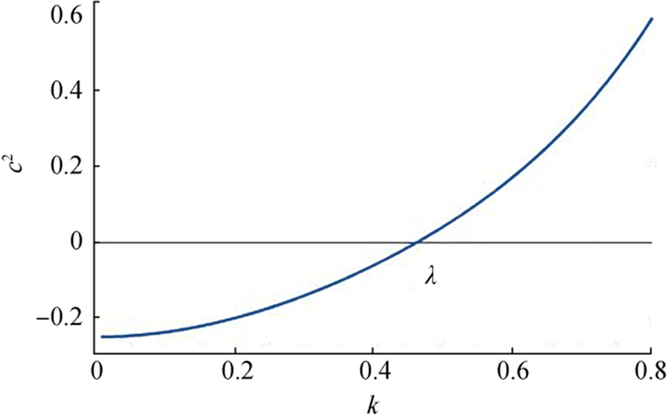
When $ Gh \lt 1 $, the graphical behavior of, $ {c}^{2} $ is shown in Figure 2. From the figure it is observed that $ {c}^{2} $ behaves well against $ k $ for small values of porosity parameter which may further indicate for small porosity parameter, the size of the pores in the sea bed is small.
There is a root $ k=\lambda $ and from graphical view $ {c}^{2} $ can be written as
$$ {c}^{2}=\left\{\begin{array}{c}{c}_{1}^{2} for k\ge \lambda \\ {c}_{2}^{2} for k \lt \lambda \end{array}\right. $$ So, taking Laplace inversions, we find the depression of the ice-covered surface in case of initial axially symmetric depression is obtained in the form
$$ {\widehat{\eta }}_{{D}_{(Gh \lt 1)}}=\left\{\begin{array}{c}\widehat{{\zeta }^{^{\prime}}}\left(k\right)[{cos}{c}_{1}t-1] for k\ge \lambda \\ \widehat{{\zeta }^{^{\prime}}}\left(k\right)\left[{cosh}{c}_{2}t-1\right] for k \lt \lambda \end{array}\right. $$ (28) and similarly in case of initial axially symmetric depression is obtained in the form
$$ {\widehat{\eta }}_{{I}_{(Gh \lt 1)}}=\left\{\begin{array}{c}\frac{\widehat{{F}^{^{\prime}}}\left(k\right)}{\rho (1+D{k}^{4})}[{c}_{1}{sin}{c}_{1}t] for k\ge \lambda \\ \frac{\widehat{{F}^{^{\prime}}}\left(k\right)}{\rho (1+D{k}^{4})}\left[{c}_{2}{sinh}{c}_{2}t\right] for k \lt \lambda \end{array}\right. $$ (29) Finally, taking inverse Hankel to transform the form of ice-covered surface depression in case of initial axially symmetric depression or impulse for $ Gh \lt 1 $ are given by
$$ {\eta }_{{D}_{\left(Gh \lt 1\right)}}(r,t)=\frac{1}{\sqrt{2\pi }}\left[{\int }_{0}^{\lambda }\widehat{{\zeta }^{^{\prime}}}\left(k\right)\left({cosh }{c}_{2}t-1\right)k{J}_{0}\left(kr\right){d}k+ {\int }_{\lambda }^{\infty }\widehat{{\zeta }^{^{\prime}}}\left(k\right)\left({cos} {c}_{1}t-1\right)k{J}_{0}\left(kr\right){d}k\right] $$ (30) or
$$ {\eta }_{{I}_{\left(Gh \lt 1\right)}}\left(r,t\right)=\frac{1}{\sqrt{2\pi \rho }}\left[{\int }_{0}^{\lambda }\frac{\widehat{{F}^{^{\prime}}}\left(k\right)}{\rho \left(1+D{k}^{4}\right)}\left({c}_{2}{sinh}{c}_{2}t\right) k{J}_{0}\left(kr\right){d}k+ {\int }_{\lambda }^{\infty }\frac{\widehat{{F}^{^{\prime}}}\left(k\right)}{\rho \left(1+D{k}^{4}\right)}\left({c}_{1}{sin}{c}_{1}t\right)k{J}_{0}\left(kr\right){d}k\right] $$ (31) 3.2 Case B ($ Gh\ge 1 $)
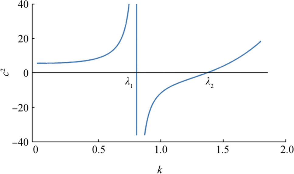
When $ Gh\ge 1 $, the graphical behavior of $ {c}^{2} $ is shown in Figure 3. The denominator of $ {c}^{2} $ has a root of $ k={\lambda }_{1} $ and numerator of $ {c}^{2} $ and has a root $ k={\lambda }_{2} $. From the figure, it is observed that $ {c}^{2} $ has a singularity in the domain for a larger value of porosity parameter, which may further indicate that for large porosity parameter the size of the pores in the sea bed is increasing slidely.
So, from graphical view $ {c}^{2} $ can be written as
$$ {c}^{2}=\left\{\begin{array}{c}{d}_{1}^{2} for 0 \lt k \lt {\lambda }_{1}-{\epsilon }_{1},\\ {-d}_{2}^{2} for {\lambda }_{1}+{\epsilon }_{1} \lt k \lt {\lambda }_{2}\\ {d}_{3}^{2} for {\lambda }_{2} \lt k \lt \infty \end{array}\right. $$ where $ {\epsilon }_{1} $ is an arbitrary small positive real number.
So, taking Laplace inversions using the Cauchy principal value of integrals, we find the depression of the ice-covered surface in case of initial axially symmetric depression is obtained in the form
$$ {\widehat{\eta }}_{{D}_{(Gh\ge 1)}}=\left\{\begin{array}{c}\widehat{{\zeta }^{^{\prime}}}\left(k\right)[{cos}{d}_{1}t-1] for 0 \lt k \lt {\lambda }_{1}-{\epsilon }_{1}\\ \widehat{{\zeta }^{^{\prime}}}\left(k\right)[{cosh}{d}_{2}t-1] for {\lambda }_{1}+{\epsilon }_{1} \lt k \lt {\lambda }_{2}\\ \widehat{{\zeta }^{^{\prime}}}\left(k\right)[{cos}{d}_{3}t-1] for {\lambda }_{2} \lt k \lt \infty \end{array}\right. $$ and similarly in case of initial axially symmetric depression is obtained in the form
$$ {\widehat{\eta }}_{{I}_{(Gh\ge 1)}}=\left\{\begin{array}{c}\frac{\widehat{{F}^{^{\prime}}}\left(k\right)}{\rho (1+D{k}^{4})}[{d}_{1}{sin}{d}_{1}t] for 0 \lt k \lt {\lambda }_{1}-{\epsilon }_{1}\\ -\frac{\widehat{{F}^{^{\prime}}}\left(k\right)}{\rho (1+D{k}^{4})}[{d}_{2}{sinh}{d}_{2}t] for {\lambda }_{1}+{\epsilon }_{1} \lt k \lt {\lambda }_{2}\\ \frac{\widehat{{F}^{^{\prime}}}\left(k\right)}{\rho (1+D{k}^{4})}[{d}_{3}{sin}{d}_{3}t] for {\lambda }_{2} \lt k \lt \infty \end{array}\right. $$ Finally, taking inverse Hankel to transform the form of ice-covered surface depression in case of initial axially symmetric depression or impulse for $ Gh\ge 1 $ are given by
$$ {{\eta }_{D}}_{\left(Gh\ge 1\right)}\left(r,t\right)=\frac{1}{\sqrt{2\pi }}\underset{{\epsilon }_{1}\to 0}{{lim}}\left[{\int }_{0}^{{\lambda }_{1}-{\epsilon }_{1}}\widehat{{\zeta }^{^{\prime}}}\left(k\right)\left({cos} {d}_{1}t-1\right)k{J}_{0}\left(kr\right){d}k+{\int }_{{\lambda }_{1}+{\epsilon }_{1}}^{{\lambda }_{2}}\widehat{{\zeta }^{^{\prime}}}\left(k\right)\left({cosh }{d}_{2}t-1\right)k{J}_{0}\left(kr\right){d}k+{\int }_{{\lambda }_{2}}^{\infty }\widehat{{\zeta }^{^{\prime}}}\left(k\right)\left({cos} {d}_{3}t-1\right)k{J}_{0}\left(kr\right){d}k\right] $$ (32) or
$$ {{\eta }_{D}}_{\left(Gh\ge 1\right)}\left(r,t\right)=\frac{1}{\sqrt{2\pi }}\underset{{\epsilon }_{1}\to 0}{{lim}}\left[{\int }_{0}^{{\lambda }_{1}-{\epsilon }_{1}}\frac{\widehat{{F}^{^{\prime}}}\left(k\right)}{\rho (1+D{k}^{4} )}{(d}_{1}{sin}{d}_{1}t)k{J}_{0}\left(kr\right){d}k+{\int }_{{\lambda }_{1}+{\epsilon }_{1}}^{{\lambda }_{2}}\frac{\widehat{{F}^{^{\prime}}}\left(k\right)}{\rho (1+D{k}^{4} )}{(d}_{2}{sinh}{d}_{2}t)k{J}_{0}\left(kr\right){d}k+{\int }_{{\lambda }_{2}}^{\infty }\frac{\widehat{{F}^{^{\prime}}}\left(k\right)}{\rho (1+D{k}^{4} )}{(d}_{3}{sin}{d}_{3}t)k{J}_{0}\left(kr\right){d}k\right] $$ (33) 4 Asymptotic Expansion of Initial Depression of the Ice-covered Surface: Stationary Phase Method
The integrands of the above integrals are oscillatory in nature and sometimes the asymptotic forms of the integrals are more suitable for certain physical applications. Here, the integrals will be evaluated asymptotically for large distance $ {\boldsymbol{r}} $ and time $ {\boldsymbol{t}} $ such that $ \frac{{\boldsymbol{r}}}{{\boldsymbol{t}}} $ is finite, by the application of the method of the stationary phase.
4.1 Case A $ ({\boldsymbol{G}}{\boldsymbol{h}} \lt 1) $
We use the integral representation of $ {{\boldsymbol{J}}}_{0}\left({\boldsymbol{k}}{\boldsymbol{r}}\right) $ as
$$ {{\boldsymbol{J}}}_{0}({\boldsymbol{k}}{\boldsymbol{r}})=\frac{2}{{\boldsymbol{\pi}}}{\int }_{0}^{\frac{{\boldsymbol{\pi}}}{2}}{c}{o}{s}\left({\boldsymbol{k}}{\boldsymbol{r}}\boldsymbol{ }{c}{o}{s}{\boldsymbol{\theta}}\right)\boldsymbol{ }{d}{\boldsymbol{\theta}} $$ (34) in Eqs. (30) and (31), so that the integral form of the ice-covered surface depression becomes a double integral, and we use the method of stationary phase twice. Applying the method of stationary phase to the integral (34) $ {{\boldsymbol{J}}}_{0}({\boldsymbol{k}}{\boldsymbol{r}}) $ can be approximated as
$$ {{\boldsymbol{J}}}_{0}\left({\boldsymbol{k}}{\boldsymbol{r}}\right)\approx {\left(\frac{2}{{\boldsymbol{\pi}}{\boldsymbol{k}}{\boldsymbol{r}}}\right)}^\frac{1}{2}{c}{o}{s}\boldsymbol{ }\left({\boldsymbol{k}}{\boldsymbol{r}}-\frac{{\boldsymbol{\pi}}}{4}\right) $$ (35) Putting the approximation of $ {{\boldsymbol{J}}}_{0}({\boldsymbol{k}}{\boldsymbol{r}}) $ on Eq. (30) we have
$$ {{\boldsymbol{\eta}}}_{{{\boldsymbol{D}}}_{\left({\boldsymbol{G}}{\boldsymbol{h}} \lt 1\right)}}\left({\boldsymbol{r}},{\boldsymbol{t}}\right)=\frac{1}{{\boldsymbol{\pi}}}\left[{\int }_{0}^{{\boldsymbol{\lambda}}}\widehat{{{\boldsymbol{\zeta}}}^{\boldsymbol{^{\prime}}}}\left({\boldsymbol{k}}\right)\left({c}{o}{s}{h}\boldsymbol{ }{{\boldsymbol{c}}}_{2}{\boldsymbol{t}}-1\right){\left(\frac{{\boldsymbol{k}}}{{\boldsymbol{r}}}\right)}^\frac{1}{2}{c}{o}{s}\boldsymbol{ }\left({\boldsymbol{k}}{\boldsymbol{r}}-\frac{{\boldsymbol{\pi}}}{4}\right){d}{\boldsymbol{k}}\right.+\left.{\int }_{{\boldsymbol{\lambda}}}^{\boldsymbol{\infty }}\widehat{{{\boldsymbol{\zeta}}}^{\boldsymbol{^{\prime}}}}\left({\boldsymbol{k}}\right)\left({c}{o}{s}\boldsymbol{ }{{\boldsymbol{c}}}_{1}{\boldsymbol{t}}-1\right){\left(\frac{{\boldsymbol{k}}}{{\boldsymbol{r}}}\right)}^\frac{1}{2}{c}{o}{s}\boldsymbol{ }\left({\boldsymbol{k}}{\boldsymbol{r}}-\frac{{\boldsymbol{\pi}}}{4}\right){d}{\boldsymbol{k}}\right]\\ \;\;\;\;\;\;\;\;\;\;\;\;\;\;\;\;\;\;\;\;\;\;\;\;={{\boldsymbol{I}}}_{1}+{{\boldsymbol{I}}}_{2}+{{\boldsymbol{I}}}_{3}+{{\boldsymbol{I}}}_{4} ({say}) $$ where
$$ {{\boldsymbol{I}}}_{1}=\frac{1}{{\boldsymbol{\pi}}}{\int }_{0}^{{\boldsymbol{\lambda}}}\widehat{{{\boldsymbol{\zeta}}}^{\boldsymbol{^{\prime}}}}\left({\boldsymbol{k}}\right){c}{o}{s}{h}\boldsymbol{ }{{\boldsymbol{c}}}_{2}{\boldsymbol{t}}{\left(\frac{{\boldsymbol{k}}}{{\boldsymbol{r}}}\right)}^\frac{1}{2}{c}{o}{s}\boldsymbol{ }\left({\boldsymbol{k}}{\boldsymbol{r}}-\frac{{\boldsymbol{\pi}}}{4}\right){d}{\boldsymbol{k}} $$ $$ {{\boldsymbol{I}}}_{2}=-\frac{1}{{\boldsymbol{\pi}}}{\int }_{0}^{{\boldsymbol{\lambda}}}\widehat{{{\boldsymbol{\zeta}}}^{\boldsymbol{^{\prime}}}}\left({\boldsymbol{k}}\right){\left(\frac{{\boldsymbol{k}}}{{\boldsymbol{r}}}\right)}^\frac{1}{2}{c}{o}{s}\boldsymbol{ }\left({\boldsymbol{k}}{\boldsymbol{r}}-\frac{{\boldsymbol{\pi}}}{4}\right){d}{\boldsymbol{k}} $$ $$ {{\boldsymbol{I}}}_{3}=\frac{1}{{\boldsymbol{\pi}}}{\int }_{{\boldsymbol{\lambda}}\boldsymbol{ }}^{\boldsymbol{\infty }}\widehat{{{\boldsymbol{\zeta}}}^{\boldsymbol{^{\prime}}}}\left({\boldsymbol{k}}\right){c}{o}{s}\boldsymbol{ }{{\boldsymbol{c}}}_{1}{\boldsymbol{t}}{\left(\frac{{\boldsymbol{k}}}{{\boldsymbol{r}}}\right)}^\frac{1}{2}{c}{o}{s}\boldsymbol{ }\left({\boldsymbol{k}}{\boldsymbol{r}}-\frac{{\boldsymbol{\pi}}}{4}\right){d}{\boldsymbol{k}} $$ $$ {{\boldsymbol{I}}}_{4}=-\frac{1}{{\boldsymbol{\pi}}}{\int }_{0}^{{\boldsymbol{\lambda}}}\widehat{{{\boldsymbol{\zeta}}}^{\boldsymbol{^{\prime}}}}\left({\boldsymbol{k}}\right){\left(\frac{{\boldsymbol{k}}}{{\boldsymbol{r}}}\right)}^\frac{1}{2}{c}{o}{s}\boldsymbol{ }\left({\boldsymbol{k}}{\boldsymbol{r}}-\frac{{\boldsymbol{\pi}}}{4}\right){d}{\boldsymbol{k}} $$ The integral $ {{\boldsymbol{I}}}_{1} $ does not contribute to $ {\boldsymbol{\eta}}({\boldsymbol{r}},{\boldsymbol{t}}) $ as given in Kundu and Mandal (2019). Also, the integrals $ {{\boldsymbol{I}}}_{2} $ and $ {{\boldsymbol{I}}}_{4} $ have no stationary points in the range of the integration so they do not yield any contribution to $ {\boldsymbol{\eta}}({\boldsymbol{r}},{\boldsymbol{t}}) $. Only contribution comes from the integral $ {{\boldsymbol{I}}}_{3} $ to $ {\boldsymbol{\eta}}({\boldsymbol{r}},{\boldsymbol{t}}) $. Now, $ {{\boldsymbol{I}}}_{3} $ can be written as
$$ {{\boldsymbol{I}}}_{3}=\frac{1}{2{\boldsymbol{\pi}}}{\int }_{{\boldsymbol{\lambda}}}^{\boldsymbol{\infty }}\widehat{{{\boldsymbol{\zeta}}}^{\boldsymbol{^{\prime}}}}\left({\boldsymbol{k}}\right){\left(\frac{{\boldsymbol{k}}}{{\boldsymbol{r}}}\right)}^\frac{1}{2}[{c}{o}{s}\left({{\boldsymbol{c}}}_{1}{\boldsymbol{t}}+{\boldsymbol{k}}{\boldsymbol{r}}-\frac{{\boldsymbol{\pi}}}{4}\right)+{c}{o}{s}\left({{\boldsymbol{c}}}_{1}{\boldsymbol{t}}-{\boldsymbol{k}}{\boldsymbol{r}}+\frac{{\boldsymbol{\pi}}}{4}\right)]{d}{\boldsymbol{k}}\\ =\frac{1}{2{\boldsymbol{\pi}}}{R}{e}{\int }_{{\boldsymbol{\lambda}}}^{\boldsymbol{\infty }}\widehat{{{\boldsymbol{\zeta}}}^{\boldsymbol{^{\prime}}}}\left({\boldsymbol{k}}\right){\left(\frac{{\boldsymbol{k}}}{{\boldsymbol{r}}}\right)}^\frac{1}{2}\left[{{e}}^{{i}{\boldsymbol{t}}\left({{\boldsymbol{c}}}_{1}+{\boldsymbol{k}}\frac{{\boldsymbol{r}}}{{\boldsymbol{t}}}-\frac{{\boldsymbol{\pi}}}{4{\boldsymbol{t}}}\right)}+{{e}}^{{i}{\boldsymbol{t}}\left({{\boldsymbol{c}}}_{1}-{\boldsymbol{k}}\frac{{\boldsymbol{r}}}{{\boldsymbol{t}}}-\frac{{\boldsymbol{\pi}}}{4{\boldsymbol{t}}}\right)}\right]{d}{\boldsymbol{k}}\\ ={{\boldsymbol{J}}}_{1}+{{\boldsymbol{J}}}_{2} ({say}) $$ where
$$ {{\boldsymbol{J}}}_{1}=\frac{1}{2{\boldsymbol{\pi}}}{\int }_{{\boldsymbol{\lambda}}}^{\boldsymbol{\infty }}\widehat{{{\boldsymbol{\zeta}}}^{\boldsymbol{^{\prime}}}}\left({\boldsymbol{k}}\right){\left(\frac{{\boldsymbol{k}}}{{\boldsymbol{r}}}\right)}^\frac{1}{2}{{e}}^{{i}{\boldsymbol{t}}\left({{\boldsymbol{c}}}_{1}+{\boldsymbol{k}}\frac{{\boldsymbol{r}}}{{\boldsymbol{t}}}-\frac{{\boldsymbol{\pi}}}{4{\boldsymbol{t}}}\right)}{d}{\boldsymbol{k}} $$ $$ {{\boldsymbol{J}}}_{2}=\frac{1}{2{\boldsymbol{\pi}}}{\int }_{{\boldsymbol{\lambda}}}^{\boldsymbol{\infty }}\widehat{{{\boldsymbol{\zeta}}}^{\boldsymbol{^{\prime}}}}\left({\boldsymbol{k}}\right){\left(\frac{{\boldsymbol{k}}}{{\boldsymbol{r}}}\right)}^\frac{1}{2}{{e}}^{{i}{\boldsymbol{t}}\left({{\boldsymbol{c}}}_{1}-{\boldsymbol{k}}\frac{{\boldsymbol{r}}}{{\boldsymbol{t}}}-\frac{{\boldsymbol{\pi}}}{4{\boldsymbol{t}}}\right)}{d}{\boldsymbol{k}} $$ Now, $ {{\boldsymbol{J}}}_{1} $ does not contribute to $ {{\boldsymbol{I}}}_{3} $ as the phase function has no stationary point in the range of the integration and $ {{\boldsymbol{J}}}_{2} $ can be written in the form of
$$ {{\boldsymbol{J}}}_{2}=\frac{1}{2{\boldsymbol{\pi}}}{\int }_{{\boldsymbol{\lambda}}}^{\boldsymbol{\infty }}{\boldsymbol{\chi}}\left({\boldsymbol{k}},{\boldsymbol{t}}\right){{e}}^{{i}{\boldsymbol{t}}{\boldsymbol{\psi}}({\boldsymbol{k}})}{d}{\boldsymbol{k}} $$ where $ {\boldsymbol{\chi}}({\boldsymbol{k}},{\boldsymbol{t}})=\widehat{{{\boldsymbol{\zeta}}}^{{^{\prime}}}}\left({\boldsymbol{k}}\right){\left(\frac{{\boldsymbol{k}}}{{\boldsymbol{r}}}\right)}^\frac{1}{2} {a}{n}{d} {\boldsymbol{\psi}}({\boldsymbol{k}})={{\boldsymbol{c}}}_{1}-{\boldsymbol{k}}\frac{{\boldsymbol{r}}}{{\boldsymbol{t}}}+\frac{{\boldsymbol{\pi}}}{4{\boldsymbol{t}}} $
When $ {\boldsymbol{t}} $ is large, the function $ {e}{x}{p}\{{i}{\boldsymbol{t}}{\boldsymbol{\psi}}({\boldsymbol{k}})\} $ oscillates rapidly as $ {\boldsymbol{k}} $ changes. Hence, the largest contributions to the integral arises from the neighborhood of the points where $ {\boldsymbol{\psi}}\boldsymbol{^{\prime}}({\boldsymbol{k}})=0 $. Now, $ {\boldsymbol{\psi}}\boldsymbol{^{\prime}}({\boldsymbol{k}})={{\boldsymbol{c}}}_{1}\boldsymbol{^{\prime}}({\boldsymbol{k}})-\frac{{\boldsymbol{r}}}{{\boldsymbol{t}}} $ where
$$ {{\boldsymbol{c}}}_{1}\boldsymbol{^{\prime}}({\boldsymbol{k}})={\left(2{{\boldsymbol{c}}}_{1}\left({\boldsymbol{k}}\right)\right)}^{-1}\left[-\frac{1+5{\boldsymbol{D}}{{\boldsymbol{k}}}^{4}}{{\boldsymbol{\mu}}\left({\boldsymbol{k}}\right)-{\boldsymbol{\epsilon}}{\boldsymbol{k}}}+\frac{{\boldsymbol{k}}\left(1+{\boldsymbol{D}}{{\boldsymbol{k}}}^{4}\right)}{{\left({\boldsymbol{\mu}}\left({\boldsymbol{k}}\right)-{\boldsymbol{\epsilon}}{\boldsymbol{k}}\right)}^{2}\left({\boldsymbol{G}}-{\boldsymbol{k}}{t}{a}{n}{h}\boldsymbol{ }{\boldsymbol{k}}{\boldsymbol{h}}\right)}\left[1-{\boldsymbol{G}}{\boldsymbol{h}}\boldsymbol{ }{s}{e}{c}{{h}}^{2}{\boldsymbol{k}}{\boldsymbol{h}}-{\boldsymbol{\epsilon}}\left({\boldsymbol{G}}-{\boldsymbol{k}}\boldsymbol{ }{tanh}{\boldsymbol{k}}{\boldsymbol{h}}\boldsymbol{ }\right)+\left({{\boldsymbol{k}}{\boldsymbol{h}}\boldsymbol{ }{s}{e}{c}{h}}^{2}{\boldsymbol{k}}{\boldsymbol{h}}+{t}{a}{n}{h}\boldsymbol{ }{\boldsymbol{k}}{\boldsymbol{h}}\right)\boldsymbol{ }{\boldsymbol{\mu}}\left({\boldsymbol{k}}\right)\right]\right] $$ This $ {{\boldsymbol{c}}}_{1}^{\boldsymbol{^{\prime}}}\left({\boldsymbol{k}}\right) $ is strictly increasing in $ ({\boldsymbol{\lambda}},\boldsymbol{\infty }) $ and let $ {\boldsymbol{\kappa}}=\underset{{\boldsymbol{k}}\to{\boldsymbol{\lambda}}}{{lim}}{{c}}_{1}{^{\prime}}({\boldsymbol{k}}). $ For $ \frac{{\boldsymbol{r}}}{{\boldsymbol{t}}} \gt {\boldsymbol{\kappa}},\boldsymbol{ }\boldsymbol{ }{\boldsymbol{\psi}}\boldsymbol{^{\prime}}({\boldsymbol{k}}) $ has two real roots $ {\boldsymbol{\alpha }}_{{\boldsymbol{i}}},\sim ({\boldsymbol{i}}=1,\boldsymbol{ }2) $ in $ ({\boldsymbol{\lambda}},\boldsymbol{\infty }) $. Thus applying the method of stationary phase to the integral $ {{\boldsymbol{J}}}_{2} $ we obtain
$$ {{{\boldsymbol{\eta}}}_{{\boldsymbol{D}}}}_{{\boldsymbol{G}}{\boldsymbol{h}} \lt 1}\left({\boldsymbol{r}},{\boldsymbol{t}}\right)=\frac{1}{2{\boldsymbol{\pi}}}\sum\limits_{{\boldsymbol{i}}=1}^{2}{\boldsymbol{\chi}}\left({\boldsymbol{\alpha }}_{{\boldsymbol{i}}},{\boldsymbol{t}}\right){\left(\frac{2{\boldsymbol{\pi}}}{{\boldsymbol{t}}\left|{\boldsymbol{\psi}}\boldsymbol{^{\prime}}\boldsymbol{^{\prime}}\left({\boldsymbol{\alpha }}_{{\boldsymbol{i}}}\right)\right|}\right)}^\frac{1}{2}{c}{o}{s}\left({\boldsymbol{t}}{\boldsymbol{\psi}}\left({\boldsymbol{\alpha }}_{{\boldsymbol{i}}}\right)-\frac{{\boldsymbol{\pi}}}{4}\right) $$ (36) Similarly, in the case of initial axisymmetric impulse, the asymptotic form of the ice-covered surface depression is given by
$$ {{{\boldsymbol{\eta}}}_{{\boldsymbol{I}}}}_{{\boldsymbol{G}}{\boldsymbol{h}} \lt 1}\left({\boldsymbol{r}},{\boldsymbol{t}}\right)=\frac{1}{2{\boldsymbol{\pi}}}\sum\limits_{{\boldsymbol{i}}=1}^{2}{{\boldsymbol{\chi}}}_{1}\left({{\boldsymbol{\alpha }}_{1}}_{{\boldsymbol{i}}},{\boldsymbol{t}}\right){\left(\frac{2{\boldsymbol{\pi}}}{{\boldsymbol{t}}\left|{{\boldsymbol{\psi}}}_{1}^{\boldsymbol{^{\prime}}\boldsymbol{^{\prime}}}\left({\boldsymbol{\alpha }}_{{\boldsymbol{i}}}\right)\right|}\right)}^\frac{1}{2}{c}{o}{s}\left({\boldsymbol{t}}{{\boldsymbol{\psi}}}_{1}\left({{\boldsymbol{\alpha }}_{1}}_{{\boldsymbol{i}}}\right)-\frac{{\boldsymbol{\pi}}}{4}\right) $$ (37) where $ {{\boldsymbol{\chi}}}_{1}({\boldsymbol{k}},{\boldsymbol{t}})=\frac{{{\boldsymbol{c}}}_{1}\widehat{{{\boldsymbol{F}}}^{{^{\prime}}}}\left({\boldsymbol{k}}\right)}{{\boldsymbol{\rho}}\left(1+{\boldsymbol{D}}{{\boldsymbol{k}}}^{4}\right)}{\left(\frac{{\boldsymbol{k}}}{{\boldsymbol{r}}}\right)}^\frac{1}{2} $, $ {{\boldsymbol{\psi}}}_{1}({\boldsymbol{k}})={{\boldsymbol{c}}}_{1}-{\boldsymbol{k}}\frac{{\boldsymbol{r}}}{{\boldsymbol{t}}}+\frac{{\boldsymbol{\pi}}}{4{\boldsymbol{t}}} $, and $ {{\boldsymbol{\alpha }}_{1}}_{{\boldsymbol{i}}},({\boldsymbol{i}}=1,2) $ are the roots of $ {{\boldsymbol{\psi}}}_{1}^{{^{\prime}}}\left({\boldsymbol{k}}\right) $ in the interval $ ({\boldsymbol{\lambda}},{\infty }) $.
4.2 Case B ($ {\boldsymbol{G}}{\boldsymbol{h}}\ge 1 $)
For $ {\boldsymbol{G}}{\boldsymbol{h}}\ge 1 $ using the approximations of $ {{\boldsymbol{J}}}_{0}({\boldsymbol{k}}{\boldsymbol{r}}) $ the integral representation of $ {\boldsymbol{\eta}}({\boldsymbol{r}},{\boldsymbol{t}}) $ in case of initial axially symmetric depression is given by
$$ {\displaystyle \begin{array}{c}{{\boldsymbol{\eta}}_{\boldsymbol{D}}}_{\boldsymbol{Gh}\boldsymbol{\ge}\bf{1}}\left(\boldsymbol{r},\boldsymbol{t}\right)=\frac{\bf{1}}{\boldsymbol{\pi}}\underset{{\boldsymbol{\varepsilon}}_{\bf{1}}\boldsymbol{\to}\bf{0}}{\bf{\lim}}\left[{\int}_{\bf{0}}^{{\boldsymbol{\lambda}}_{\bf{1}}-{\boldsymbol{\epsilon}}_{\bf{1}}}\hat{{\boldsymbol{\zeta}}^{\prime }}\left(\boldsymbol{k}\right)\left(\bf{\cos}\ {\boldsymbol{d}}_{\bf{1}}\boldsymbol{t}-\bf{1}\right){\left(\frac{\boldsymbol{k}}{\boldsymbol{r}}\right)}^{\frac{\bf{1}}{\bf{2}}}\bf{\cos}\ \left(\boldsymbol{k}\boldsymbol{r}-\frac{\boldsymbol{\pi}}{\bf{4}}\right)\bf{d}\boldsymbol{k}\right.\\ {}\begin{array}{l}+{\int}_{{\boldsymbol{\lambda}}_{\bf{1}}+{\boldsymbol{\epsilon}}_{\bf{1}}}^{{\boldsymbol{\lambda}}_{\bf{2}}}\hat{{\boldsymbol{\zeta}}^{\prime }}\left(\boldsymbol{k}\right)\left(\bf{\cosh}\ {\boldsymbol{d}}_{\bf{2}}\boldsymbol{t}-\bf{1}\right){\left(\frac{\boldsymbol{k}}{\boldsymbol{r}}\right)}^{\frac{\bf{1}}{\bf{2}}}\bf{\cos}\ \left(\boldsymbol{k}\boldsymbol{r}-\frac{\boldsymbol{\pi}}{\bf{4}}\right)\bf{d}\boldsymbol{k}\\ {}\begin{array}{c}+{\int}_{\bf{0}}^{{\boldsymbol{\lambda}}_{\bf{1}}-{\boldsymbol{\epsilon}}_{\bf{1}}}\hat{{\boldsymbol{\zeta}}^{\prime }}\left(\boldsymbol{k}\right)\left(\bf{\cos}\ {\boldsymbol{d}}_{\bf{1}}\boldsymbol{t}-\bf{1}\right){\left(\frac{\boldsymbol{k}}{\boldsymbol{r}}\right)}^{\frac{\bf{1}}{\bf{2}}}\bf{\cos}\ \left(\boldsymbol{k}\boldsymbol{r}-\frac{\boldsymbol{\pi}}{\bf{4}}\right)\bf{d}\boldsymbol{k}\\ {}\left.+{\int}_{{\boldsymbol{\lambda}}_{\bf{2}}}^{\boldsymbol{\infty}}\hat{{\boldsymbol{\zeta}}^{\prime }}\left(\boldsymbol{k}\right)\left(\bf{\cos}\ {\boldsymbol{d}}_{\bf{3}}\boldsymbol{t}-\bf{1}\right){\left(\frac{\boldsymbol{k}}{\boldsymbol{r}}\right)}^{\frac{\bf{1}}{\bf{2}}}\bf{\cos}\ \left(\boldsymbol{k}\boldsymbol{r}-\frac{\boldsymbol{\pi}}{\bf{4}}\right)\bf{d}\boldsymbol{k}\ \right]\end{array}\end{array}\end{array}} $$ Here, also the only contribution comes from the integrals
$$ {{\boldsymbol{I}}}_{1}\boldsymbol{^{\prime}}=\underset{{{\boldsymbol{\epsilon}}}_{1}\to 0}{{lim}}{\int }_{0}^{{{\boldsymbol{\lambda}}}_{1}-{{\boldsymbol{\epsilon}}}_{1}}\widehat{{{\boldsymbol{\zeta}}}^{\boldsymbol{^{\prime}}}}\left({\boldsymbol{k}}\right){cos}{{\boldsymbol{d}}}_{1}{\boldsymbol{t}}{\left(\frac{{\boldsymbol{k}}}{{\boldsymbol{r}}}\right)}^\frac{1}{2}{c}{o}{s}\boldsymbol{ }\left({\boldsymbol{k}}{\boldsymbol{r}}-\frac{{\boldsymbol{\pi}}}{4}\right){d}{\boldsymbol{k}} $$ and
$$ {{\boldsymbol{I}}}_{2}\boldsymbol{^{\prime}}=\underset{{{\boldsymbol{\epsilon}}}_{1}\to 0}{{lim}}{\int }_{{{\boldsymbol{\lambda}}}_{2}}^{\boldsymbol{\infty }}\widehat{{{\boldsymbol{\zeta}}}^{\boldsymbol{^{\prime}}}}\left({\boldsymbol{k}}\right){cos}{{\boldsymbol{d}}}_{3}{\boldsymbol{t}}{\left(\frac{{\boldsymbol{k}}}{{\boldsymbol{r}}}\right)}^\frac{1}{2}{c}{o}{s}\boldsymbol{ }\left({\boldsymbol{k}}{\boldsymbol{r}}-\frac{{\boldsymbol{\pi}}}{4}\right){d}{\boldsymbol{k}} $$ Using the method of stationary phase to these integrals, the asymptotic form of the ice-covered surface depression, in case of axially symmetric impulse for $ {\boldsymbol{G}}{\boldsymbol{h}}\ge 1 $ is given by
$$ {{{\boldsymbol{\eta}}}_{{\boldsymbol{D}}}}_{{\boldsymbol{G}}{\boldsymbol{h}}\ge 1}({\boldsymbol{r}},{\boldsymbol{t}})=\frac{1}{2{\boldsymbol{\pi}}}\left[{{\boldsymbol{\chi}}}_{2}\left({\boldsymbol{\beta}},{\boldsymbol{t}}\right){\left(\frac{2{\boldsymbol{\pi}}}{{\boldsymbol{t}}\left|{{\boldsymbol{\psi}}}_{2}^{\boldsymbol{^{\prime}}\boldsymbol{^{\prime}}}\left({\boldsymbol{\beta}}\right)\right|}\right)}^\frac{1}{2}{cos}\left({\boldsymbol{t}}{{\boldsymbol{\psi}}}_{2}\left({\boldsymbol{\beta}}\right)-\frac{{\boldsymbol{\pi}}}{4}\right)\right.\\ +\left.\sum\limits_{{\boldsymbol{i}}=1}^{2}{{\boldsymbol{\chi}}}_{2}({{{\boldsymbol{\beta}}}_{1}}_{{\boldsymbol{i}}},{\boldsymbol{t}}){\left(\frac{2{\boldsymbol{\pi}}}{{\boldsymbol{t}}\left|{{\boldsymbol{\psi}}}_{3}^{\boldsymbol{^{\prime}}\boldsymbol{^{\prime}}}\left({{{\boldsymbol{\beta}}}_{1}}_{{\boldsymbol{i}}}\boldsymbol{ }\right)\right|}\right)}^\frac{1}{2}{cos}\left({\boldsymbol{t}}{{\boldsymbol{\psi}}}_{3}\left({{{\boldsymbol{\beta}}}_{1}}_{{\boldsymbol{i}}}\right)-\frac{{\boldsymbol{\pi}}}{4}\right)\right] $$ where.
$ {{\boldsymbol{\chi}}}_{2}({\boldsymbol{k}},{\boldsymbol{t}})=\widehat{{{\boldsymbol{\zeta}}}^{\boldsymbol{^{\prime}}}}\left({\boldsymbol{k}}\right){\left(\frac{{\boldsymbol{k}}}{{\boldsymbol{r}}}\right)}^\frac{1}{2},\boldsymbol{ }{{\boldsymbol{\psi}}}_{2}({\boldsymbol{k}})={{\boldsymbol{d}}}_{1}-{\boldsymbol{k}}\frac{{\boldsymbol{r}}}{{\boldsymbol{t}}}+\frac{{\boldsymbol{\pi}}}{4{\boldsymbol{t}}},\boldsymbol{ }{{\boldsymbol{\psi}}}_{3}({\boldsymbol{k}})={{\boldsymbol{d}}}_{3}-{\boldsymbol{k}}\frac{{\boldsymbol{r}}}{{\boldsymbol{t}}}+\frac{{\boldsymbol{\pi}}}{4{\boldsymbol{t}}} $, and $ {\boldsymbol{\beta}},\boldsymbol{ }{{{\boldsymbol{\beta}}}_{1}}_{{\boldsymbol{i}}},({\boldsymbol{i}}=1,2) $ are the roots of $ {{\boldsymbol{\psi}}}_{2}\boldsymbol{^{\prime}}({\boldsymbol{k}}) $ and $ {{\boldsymbol{\psi}}}_{3}\boldsymbol{^{\prime}}({\boldsymbol{k}}) $ in the respective range of integrations.
Similarly, in the case of initial axisymmetric impulse, the asymptotic form of the ice-covered surface depression for $ {\boldsymbol{G}}{\boldsymbol{h}}\ge 1 $ is given by
$$ {{{\boldsymbol{\eta}}}_{{\boldsymbol{I}}}}_{{\boldsymbol{G}}{\boldsymbol{h}}\ge 1}({\boldsymbol{r}},{\boldsymbol{t}})=\frac{1}{2{\boldsymbol{\pi}}}\left[{{\boldsymbol{\chi}}}_{3}\left({\boldsymbol{\gamma}},{\boldsymbol{t}}\right){\left(\frac{2{\boldsymbol{\pi}}}{{\boldsymbol{t}}\left|{{\boldsymbol{\psi}}}_{2}^{\boldsymbol{^{\prime}}\boldsymbol{^{\prime}}}\left({\boldsymbol{\gamma}}\right)\right|}\right)}^\frac{1}{2}{cos}\left({\boldsymbol{t}}{{\boldsymbol{\psi}}}_{2}\left({\boldsymbol{\gamma}}\right)-\frac{{\boldsymbol{\pi}}}{4}\right)\right.\\ +\left.\sum\limits_{{\boldsymbol{i}}=1}^{2}{{\boldsymbol{\chi}}}_{4}({{{\boldsymbol{\gamma}}}_{1}}_{{\boldsymbol{i}}},{\boldsymbol{t}}){\left(\frac{2{\boldsymbol{\pi}}}{{\boldsymbol{t}}\left|{{\boldsymbol{\psi}}}_{3}^{\boldsymbol{^{\prime}}\boldsymbol{^{\prime}}}\left({{{\boldsymbol{\gamma}}}_{1}}_{{\boldsymbol{i}}}\boldsymbol{ }\right)\right|}\right)}^\frac{1}{2}{cos}\left({\boldsymbol{t}}{{\boldsymbol{\psi}}}_{3}\left({{{\boldsymbol{\gamma}}}_{1}}_{{\boldsymbol{i}}}\right)-\frac{{\boldsymbol{\pi}}}{4}\right)\right] $$ where.
$ {{\boldsymbol{\chi}}}_{3}\left({\boldsymbol{k}},{\boldsymbol{t}}\right)=\frac{{{\boldsymbol{d}}}_{1}\widehat{{{\boldsymbol{F}}}^{\boldsymbol{^{\prime}}}}\left({\boldsymbol{k}}\right)}{{\boldsymbol{\rho}}\left(1+{\boldsymbol{D}}{{\boldsymbol{k}}}^{4}\right)}{\left(\frac{{\boldsymbol{k}}}{{\boldsymbol{r}}}\right)}^\frac{1}{2},\boldsymbol{ }{{\boldsymbol{\psi}}}_{2}\left({\boldsymbol{k}}\right)={{\boldsymbol{d}}}_{1}-{\boldsymbol{k}}\frac{{\boldsymbol{r}}}{{\boldsymbol{t}}}+\frac{{\boldsymbol{\pi}}}{4{\boldsymbol{t}}},\boldsymbol{ }{{\boldsymbol{\chi}}}_{4}\left({\boldsymbol{k}},{\boldsymbol{t}}\right)=\frac{{{\boldsymbol{d}}}_{3}\widehat{{{\boldsymbol{F}}}^{\boldsymbol{^{\prime}}}}\left({\boldsymbol{k}}\right)}{{\boldsymbol{\rho}}\left(1+{\boldsymbol{D}}{{\boldsymbol{k}}}^{4}\right)}{\left(\frac{{\boldsymbol{k}}}{{\boldsymbol{r}}}\right)}^\frac{1}{2},{{\boldsymbol{\psi}}}_{3}\left({\boldsymbol{k}}\right)={{\boldsymbol{d}}}_{3}-{\boldsymbol{k}}\frac{{\boldsymbol{r}}}{{\boldsymbol{t}}}+\frac{{\boldsymbol{\pi}}}{4{\boldsymbol{t}}}, $ and $ {\boldsymbol{\gamma}},{{{\boldsymbol{\gamma}}}_{1}}_{{\boldsymbol{i}}}\boldsymbol{ },({\boldsymbol{i}}=1,2) $ are the roots of $ {{\boldsymbol{\psi}}}_{2}\boldsymbol{^{\prime}}({\boldsymbol{k}}) $ and $ {{\boldsymbol{\psi}}}_{3}\boldsymbol{^{\prime}}({\boldsymbol{k}}) $ in the respective range of integrations.
4.3 Justification of the Method of Stationary Phase
We now prove how the integrals $ {{\boldsymbol{I}}}_{1},{{\boldsymbol{I}}}_{2},{{\boldsymbol{I}}}_{4} $ have no contributions to the ice-cover surface depression. Consider the integral
$$ {{\boldsymbol{I}}}_{1}=\frac{1}{{\boldsymbol{\pi}}}{\int }_{0}^{{\boldsymbol{\lambda}}}\widehat{{{\boldsymbol{\zeta}}}^{\boldsymbol{^{\prime}}}}\left({\boldsymbol{k}}\right){c}{o}{s}{h}\left({{\boldsymbol{c}}}_{2}{\boldsymbol{t}}\right){\left(\frac{{\boldsymbol{k}}}{{\boldsymbol{r}}}\right)}^\frac{1}{2}{c}{o}{s}\left({\boldsymbol{k}}{\boldsymbol{r}}-\frac{{\boldsymbol{\pi}}}{4}\right){d}{\boldsymbol{k}} $$ which can be further written as considering $ {\boldsymbol{r}} $ as large parameter
$$ {{\boldsymbol{I}}}_{1}={R}{e}\left[\frac{1}{{\boldsymbol{\pi}}}{\int }_{0}^{{\boldsymbol{\lambda}}}\widehat{{{\boldsymbol{\zeta}}}^{\boldsymbol{^{\prime}}}}\left({\boldsymbol{k}}\right){c}{o}{s}{h}\left({{\boldsymbol{c}}}_{2}{\boldsymbol{t}}\right){\left(\frac{{\boldsymbol{k}}}{{\boldsymbol{r}}}\right)}^\frac{1}{2}{{e}}^{{i}{\boldsymbol{r}}\left({\boldsymbol{k}}-\frac{{\boldsymbol{\pi}}}{4{\boldsymbol{r}}}\right)}{d}{\boldsymbol{k}}\right]={R}{e}\left[\frac{1}{{\boldsymbol{\pi}}}{\int }_{0}^{{\boldsymbol{\lambda}}}{\boldsymbol{\delta}}\left({\boldsymbol{k}}\right){{e}}^{{i}{\boldsymbol{r}}{\boldsymbol{\omega}}\left({\boldsymbol{k}}\right)}{d}{\boldsymbol{k}}\right] $$ where $ {\boldsymbol{\delta}}({\boldsymbol{k}})=\widehat{{{\boldsymbol{\zeta}}}^{\boldsymbol{^{\prime}}}}\left({\boldsymbol{k}}\right){c}{o}{s}{h}\left({{\boldsymbol{c}}}_{2}{\boldsymbol{t}}\right){\left(\frac{{\boldsymbol{k}}}{{\boldsymbol{r}}}\right)}^\frac{1}{2} $ and the phase function $ {\boldsymbol{\omega}}({\boldsymbol{k}})={\boldsymbol{k}}-\frac{{\boldsymbol{\pi}}}{4{\boldsymbol{r}}}. $ Now these two functions are regular analytic in the range of integration and $ {{\boldsymbol{\omega}}}^{\boldsymbol{^{\prime}}}\left({\boldsymbol{k}}\right)=1\ne \boldsymbol{ }0 $ in the range of integration. So we may write
$$ {{\boldsymbol{I}}}_{1}={\int }_{0}^{{\boldsymbol{\lambda}}}\frac{{\boldsymbol{\delta}}\left({\boldsymbol{k}}\right)}{{i}{\boldsymbol{r}}{{\boldsymbol{\omega}}}^{\boldsymbol{^{\prime}}}\left({\boldsymbol{k}}\right)}\frac{{d}}{{d}{\boldsymbol{k}}}\left({{e}}^{{i}{\boldsymbol{r}}{\boldsymbol{\omega}}\left({\boldsymbol{k}}\right)}\right){d}{\boldsymbol{k}} $$ Integration by parts leads to the result
$$ {{\boldsymbol{I}}}_{1}=\frac{{\boldsymbol{\delta}}({\boldsymbol{\lambda}})}{{i}{\boldsymbol{r}}}{{e}}^{{i}{\boldsymbol{r}}{\boldsymbol{\omega}}({\boldsymbol{\lambda}})}-\frac{1}{{i}{\boldsymbol{r}}}{\int }_{0}^{{\boldsymbol{\lambda}}}{{e}}^{{i}{\boldsymbol{r}}{\boldsymbol{\omega}}\left({\boldsymbol{\lambda}}\right)}\frac{{d}}{{d}{\boldsymbol{k}}}\left({\boldsymbol{\delta}}\left({\boldsymbol{k}}\right)\right){d}{\boldsymbol{k}}\le \frac{{\boldsymbol{\delta}}\left({\boldsymbol{\lambda}}\right)}{{i}{\boldsymbol{r}}}{{e}}^{{i}{\boldsymbol{r}}{\boldsymbol{\omega}}\left({\boldsymbol{\lambda}}\right)}-\frac{1}{{i}{\boldsymbol{r}}}{\int }_{0}^{{\boldsymbol{\lambda}}}|{\boldsymbol{\delta}}({\boldsymbol{k}})|{d}{\boldsymbol{k}} $$ as $ {\boldsymbol{r}}{\boldsymbol{\omega}}({\boldsymbol{k}}) $ is real and $ {{\boldsymbol{I}}}_{1} $ is bounded of order $ \frac{1}{{\boldsymbol{r}}} $. So this integral does not contribute to $ {{\boldsymbol{\eta}}}_{{\boldsymbol{D}}}({\boldsymbol{r}},{\boldsymbol{t}}) $ and by similar approach, it can be proved that $ {{\boldsymbol{I}}}_{2} $ and $ {{\boldsymbol{I}}}_{4} $ do not contribute since the integrands of these two integrals behave appropriately at $ \boldsymbol{\infty } $.
Now, consider the integral $ {{\boldsymbol{J}}}_{2} $ which makes contribution to $ {{\boldsymbol{\eta}}}_{{\boldsymbol{D}}}({\boldsymbol{r}},{\boldsymbol{t}}) $.
So, $ {{\boldsymbol{J}}}_{2}=\frac{1}{2{\boldsymbol{\pi}}}{\int }_{{\boldsymbol{\lambda}}}^{\boldsymbol{\infty }}{\boldsymbol{\chi}}\left({\boldsymbol{k}},{\boldsymbol{t}}\right){{e}}^{{i}{\boldsymbol{t}}{\boldsymbol{\psi}}\left({\boldsymbol{k}}\right)}{d}{\boldsymbol{k}} $where $ {\boldsymbol{\chi}}({\boldsymbol{k}},{\boldsymbol{t}})=\widehat{{{\boldsymbol{\zeta}}}^{\boldsymbol{^{\prime}}}}\left({\boldsymbol{k}}\right){\left(\frac{{\boldsymbol{k}}}{{\boldsymbol{r}}}\right)}^\frac{1}{2} $ and $ {\boldsymbol{\psi}}({\boldsymbol{k}})={{\boldsymbol{c}}}_{1}-{\boldsymbol{k}}\frac{{\boldsymbol{r}}}{{\boldsymbol{t}}}+\frac{{\boldsymbol{\pi}}}{4{\boldsymbol{t}}}. $ Since $ {\boldsymbol{\psi}}\boldsymbol{^{\prime}}({\boldsymbol{k}}) $ is a regular in the range of integration so the zeros $ {\boldsymbol{\alpha }}_{{\boldsymbol{i}}},({\boldsymbol{i}}=1,\boldsymbol{ }2) $ of $ {\boldsymbol{\psi}}\boldsymbol{^{\prime}}({\boldsymbol{k}}) $ are isolated. Without loss of generality let $ {\boldsymbol{\lambda}} \lt {\boldsymbol{\alpha }}_{1} \lt {\boldsymbol{\alpha }}_{2} $. So the range of integration can be divided into four parts of which three intervals $ \left({\boldsymbol{\lambda}},{\boldsymbol{\alpha }}_{1}-{{\boldsymbol{\epsilon}}}^{\boldsymbol{^{\prime}}}\right),\left(\boldsymbol{\alpha}_{1}+\mathbf{\epsilon}^{\prime}, \boldsymbol{\alpha}_{2}-\boldsymbol{\epsilon}^{\prime}\right)$, and $ \left({\boldsymbol{\alpha }}_{2}+{{\boldsymbol{\epsilon}}}^{\boldsymbol{^{\prime}}},\boldsymbol{ }\boldsymbol{\infty }\right) $ contain no stationary points so that their contribution become an order of $ \frac{1}{{\boldsymbol{t}}} $. The other small intervals $ ({\boldsymbol{\alpha }}_{1}-{{\boldsymbol{\epsilon}}}^{\boldsymbol{^{\prime}}},\boldsymbol{ }{\boldsymbol{\alpha }}_{1}+{\boldsymbol{\epsilon}}\boldsymbol{^{\prime}}) $ and $ ({\boldsymbol{\alpha }}_{2}-{\boldsymbol{\epsilon}}\boldsymbol{^{\prime}},{\boldsymbol{\alpha }}_{2}+{\boldsymbol{\epsilon}}\boldsymbol{^{\prime}}) $ contains only one stationary point. Thus $ {\boldsymbol{\psi}}\boldsymbol{^{\prime}}({\boldsymbol{k}})=0 $ only at $ {\boldsymbol{k}}={\boldsymbol{\alpha }}_{{\boldsymbol{i}}} $ and $ {\boldsymbol{\psi}}\boldsymbol{^{\prime}}\boldsymbol{^{\prime}}({\boldsymbol{\alpha }}_{{\boldsymbol{i}}}) \gt 0 $ in the given interval. Consider a positive $ {\boldsymbol{\epsilon}} $ such that $ {\boldsymbol{\epsilon}}\le{\boldsymbol{\epsilon}}\boldsymbol{^{\prime}} $ then $ {{\boldsymbol{J}}}_{2} $ becomes
$$ {{\boldsymbol{J}}}_{2}=\frac{1}{2{\boldsymbol{\pi}}}\sum\limits_{{\boldsymbol{i}}=1}^{2}{\int }_{{\boldsymbol{\alpha }}_{{\boldsymbol{i}}}-{{\boldsymbol{\epsilon}}}^{\boldsymbol{^{\prime}}}}^{{\boldsymbol{\alpha }}_{{\boldsymbol{i}}}\boldsymbol{ }+{\boldsymbol{\epsilon}}\boldsymbol{^{\prime}}}{\boldsymbol{\chi}}\left({\boldsymbol{k}},{\boldsymbol{t}}\right){{e}}^{{i}{\boldsymbol{t}}{\boldsymbol{\psi}}({\boldsymbol{k}})}{d}{\boldsymbol{k}}\\ =\sum\limits_{{\boldsymbol{i}}=1}^{2}{\left(\frac{2{\boldsymbol{\pi}}}{{\boldsymbol{t}}{{\boldsymbol{\psi}}}^{\boldsymbol{^{\prime}}\boldsymbol{^{\prime}}}\left({\boldsymbol{\alpha }}_{{\boldsymbol{i}}}\right)}\right)}^\frac{1}{2}{\boldsymbol{\chi}}\left({\boldsymbol{\alpha }}_{{\boldsymbol{i}}},{\boldsymbol{t}}\right){{e}}^{{i}\left({\boldsymbol{t}}{\boldsymbol{\psi}}\left({\boldsymbol{\alpha }}_{{\boldsymbol{i}}}\right)+\frac{{\boldsymbol{\pi}}}{4}\right)}+{\rm O}\left(\frac{1}{{\boldsymbol{t}}}\right) $$ Now, it can be shown that a fixed segment of length $ 2{\boldsymbol{\epsilon}} $ containing $ {\boldsymbol{\alpha }}_{{\boldsymbol{i}}} $ exists such that its contribution in $ {{\boldsymbol{J}}}_{2} $, i.e., in $ {{{\boldsymbol{\eta}}}_{{\boldsymbol{D}}}}_{{\boldsymbol{G}}{\boldsymbol{h}} \lt 1}({\boldsymbol{r}},{\boldsymbol{t}}) $ independent of $ {\boldsymbol{\epsilon}} $. The value of integration is of order $ \frac{1}{\sqrt{{\boldsymbol{t}}}} $ with an error of order $ \frac{1}{{\boldsymbol{t}}} $ (Stoker 1957). Thus for large $ {\boldsymbol{t}} $ the error tends to zero and the integral $ {{\boldsymbol{J}}}_{2} $ converges. $ {{e}}^{{i}{\boldsymbol{t}}{\boldsymbol{\psi}}({\boldsymbol{k}})} $ oscillates rapidly with large value of $ {\boldsymbol{t}} $ and obviously with large $ {\boldsymbol{k}} $. Thus, the main contribution of $ {{{\boldsymbol{\eta}}}_{{\boldsymbol{D}}}}_{{\boldsymbol{G}}{\boldsymbol{h}} \lt 1}({\boldsymbol{r}},{\boldsymbol{t}}) $ comes from integral $ {{\boldsymbol{J}}}_{2} $. Similarly we can show the justification of applying the stationary phase method in Case-B, for $ {{{\boldsymbol{\eta}}}_{{\boldsymbol{D}}}}_{{\boldsymbol{G}}{\boldsymbol{h}}\ge 1}({\boldsymbol{r}},{\boldsymbol{t}}) $.
5 Numerical Results: Far-Field Behavior of Wave Amplitude
In this section, to view the far-field behavior of the generation of surface wave in the presence of ice cover and porous bottom, the nondimensional asymptotic form of $ {\boldsymbol{\eta}}({\boldsymbol{r}},{\boldsymbol{t}}) $ is depicted graphically against $ {\boldsymbol{r}} $ for fixed $ {\boldsymbol{t}} $ and against $ {\boldsymbol{t}} $ for fixed $ {\boldsymbol{r}} $ in some figures for different values of porosity parameter and ice-cover parameters.
5.1 Case A $ ({\boldsymbol{G}}{\boldsymbol{h}} \lt 1) $
5.1.1 Initial Depression
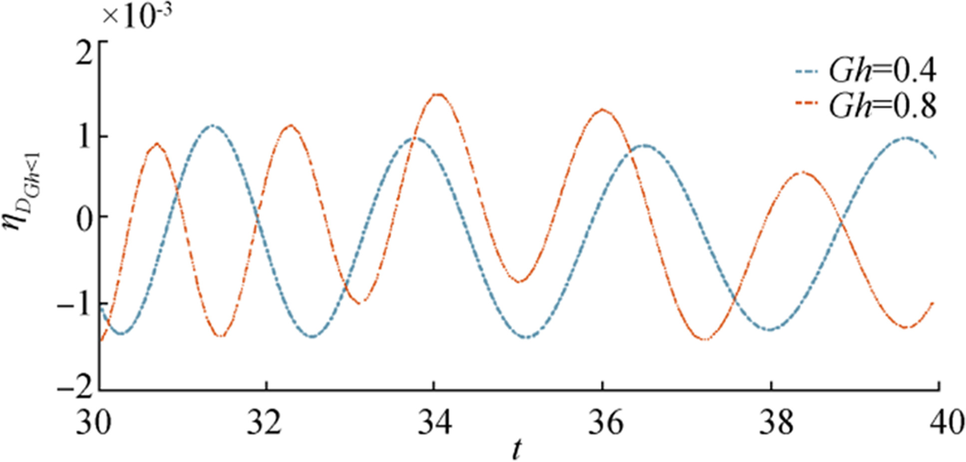
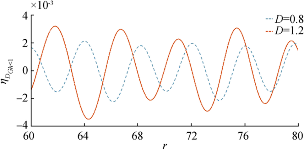
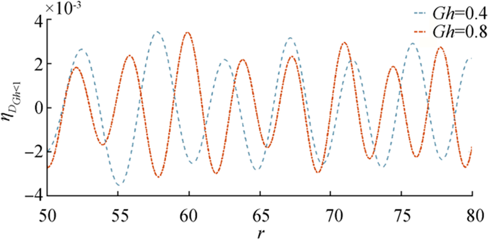
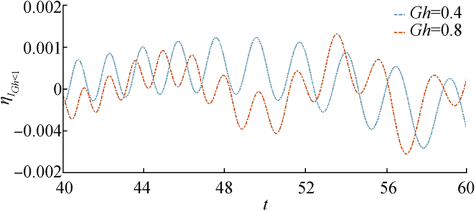
We consider the initial axially symmetric depression $ {\boldsymbol{\zeta}}\boldsymbol{^{\prime}}({\boldsymbol{r}}) $ of the ice-covered surface as a Dirac delta function $ \widehat{{\boldsymbol{\zeta}}}\boldsymbol{^{\prime}}({\boldsymbol{k}})=\frac{1}{2{\boldsymbol{\pi}}} $. Actually, the delta function is defined mathematically to provide a physical phenomenon that occurs in an extremely short period of time and is too short to be measured with an extremely large amplitude. Ice-cover surface depression $ {{{\boldsymbol{\eta}}}_{{\boldsymbol{D}}}}_{({\boldsymbol{G}}{\boldsymbol{h}} \lt 1)}({\boldsymbol{r}},{\boldsymbol{t}}) $ is plotted in Figures 4, 5, 6, and 7 for different values of parameters.
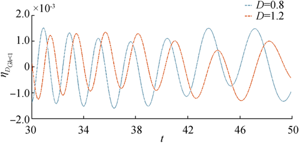
In Figure 4, $ {{\boldsymbol{\eta}}}_{{{\boldsymbol{D}}}_{{\boldsymbol{G}}{\boldsymbol{h}} \lt 1}} $ is displayed against $ {\boldsymbol{t}} $ for different values of the ice-cover parameter $ {\boldsymbol{D}} $ and fixed $ {\boldsymbol{r}},{\boldsymbol{\epsilon}},\boldsymbol{ }{\boldsymbol{G}}{\boldsymbol{h}} \lt 1 $. From Figure 4 it is observed that as $ {\boldsymbol{D}} $ increases amplitude of ice-covered surface depression decreases from which it can be concluded that as the flexural rigidity of the ice sheet increases it can offer more resistance to the surface waves so that the oscillatory nature and amplitude of waves reduces. In Figure 5, $ {{{\boldsymbol{\eta}}}_{{\boldsymbol{D}}}}_{{\boldsymbol{G}}{\boldsymbol{h}} \lt 1} $ is displayed against $ {\boldsymbol{t}} $ for different value of porosity parameter $ {\boldsymbol{G}} $ and fixed $ {\boldsymbol{r}},{\boldsymbol{\epsilon}},{\boldsymbol{D}} $.
From Figure 5, it is observed that near the time range $ {\boldsymbol{t}}=34 $ to $ 36 $ amplitude of $ {\boldsymbol{\eta}} $ is quite larger for large porosity parameter compared to other, although in the other regions amplitudes of both waves are nearly same.
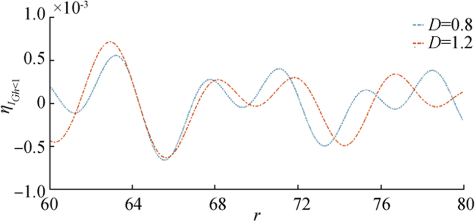
In Figure 6, wave motion has been shown against distance due to initial depression for fixed $ {\boldsymbol{t}},{\boldsymbol{\epsilon}},\boldsymbol{ }{\boldsymbol{G}}{\boldsymbol{h}} $ and different values of the ice-cover parameter. Here the increase in the flexural rigidity of the ice sheet increases the amplitude of the wave motion slightly. Figure 7 shows wave motion against distance due to initial depression for fixed $ {\boldsymbol{t}},{\boldsymbol{\epsilon}},\boldsymbol{ }{\boldsymbol{D}} $ and different values of porosity parameter less than 1. From this figure, it can be noted that near $ {\boldsymbol{r}}=60 $ amplitude wave is larger compared to the other regions for both the cases of porosity parameter.
5.1.2 Initial Impulse
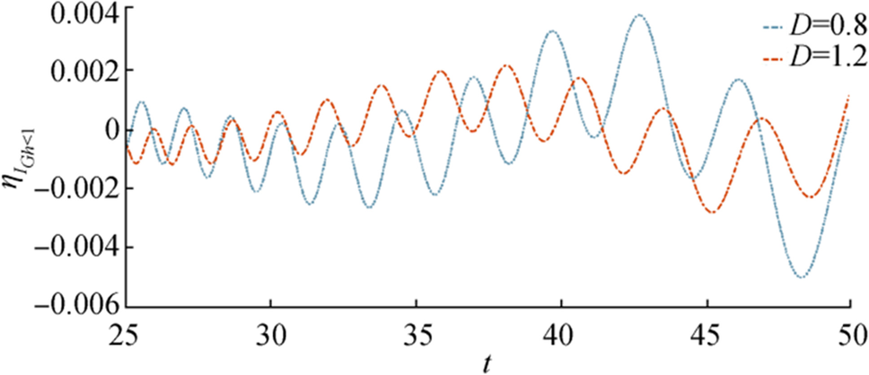
In thies case, we consider initial axially symmetric impulse $ {\boldsymbol{F}}\boldsymbol{^{\prime}}({\boldsymbol{r}}) $ as Dirac delta function or unit impulse function which is applied at a distance $ {\boldsymbol{r}} $ from the origin for an infinitesimal interval of time. Figures 8, 9, 10, and 11 have shown the behavior of $ {{{\boldsymbol{\eta}}}_{{\boldsymbol{I}}}}_{{\boldsymbol{G}}{\boldsymbol{h}} \lt 1} $ due to initial impulse for different parametric values.
In Figure 8, $ {{{\boldsymbol{\eta}}}_{{\boldsymbol{I}}}}_{{\boldsymbol{G}}{\boldsymbol{h}} \lt 1} $ is plotted against $ {\boldsymbol{t}} $ for fixed $ {\boldsymbol{r}},{\boldsymbol{\epsilon}},{\boldsymbol{G}}{\boldsymbol{h}} $ and different values of the ice-cover parameter. The amplitude of $ {{{\boldsymbol{\eta}}}_{{\boldsymbol{I}}}}_{{\boldsymbol{G}}{\boldsymbol{h}} \lt 1} $ increases as time increases and as flexural rigidity of the ice sheet increases amplitude of the surface wave decreases. Wave motion due to initial impulse for fixed $ {\boldsymbol{r}},{\boldsymbol{\epsilon}},\boldsymbol{ }{\boldsymbol{D}} $ is shown in Figure 9. From this figure, it is observed that surface waves show a highly oscillatory nature in this case.
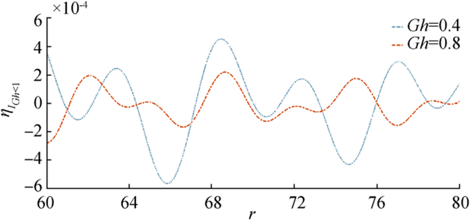
In Figure 10, $ {{{\boldsymbol{\eta}}}_{{\boldsymbol{I}}}}_{{\boldsymbol{G}}{\boldsymbol{h}} \lt 1} $ is plotted against $ {\boldsymbol{r}} $ for fixed $ {\boldsymbol{t}},{\boldsymbol{\epsilon}},{\boldsymbol{G}}{\boldsymbol{h}} $ and in Figure 11, $ {{{\boldsymbol{\eta}}}_{{\boldsymbol{I}}}}_{{\boldsymbol{G}}{\boldsymbol{h}} \lt 1} $ is plotted against $ {\boldsymbol{r}} $ for fixed $ {\boldsymbol{t}},{\boldsymbol{\epsilon}},{\boldsymbol{D}} $. From Figure 10, it is observed that the nature of surface wave is not much differing for two flexural rigidity parameters, but in the case of Figure 11, as the porosity parameter increases the amplitude of wave decreases.
5.2 Case B ($ {\boldsymbol{G}}{\boldsymbol{h}}\ge 1 $)
5.2.1 Initial Depression
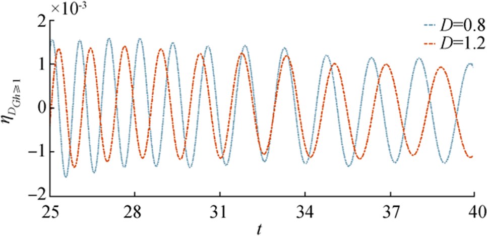
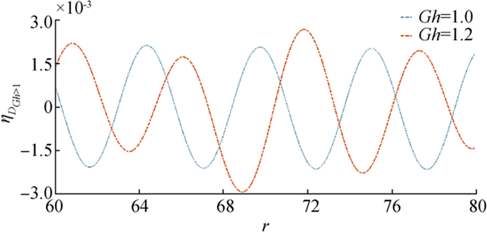
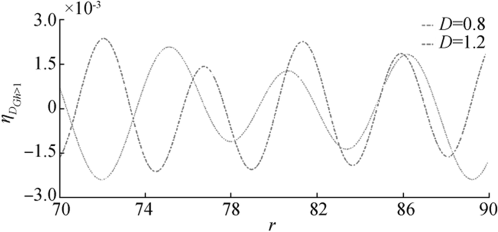
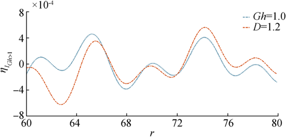
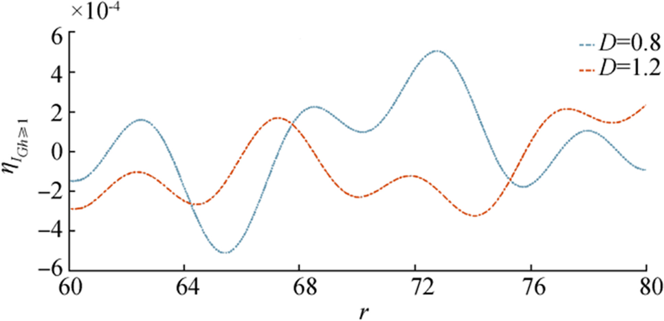
Figures 12, 13, 14, and 15 are drawn for initial depression in case of higher porosity parameter i.e., $ {\boldsymbol{G}}{\boldsymbol{h}}\ge 1 $. Figure 12 shows behavior of $ {{{\boldsymbol{\eta}}}_{{\boldsymbol{I}}}}_{{\boldsymbol{G}}{\boldsymbol{h}}\ge 1} $ for fixed $ {\boldsymbol{r}},{\boldsymbol{\epsilon}},{\boldsymbol{D}} $ and Figure 13 shows behavior of $ {{{\boldsymbol{\eta}}}_{{\boldsymbol{I}}}}_{{\boldsymbol{G}}{\boldsymbol{h}}\ge 1} $ for fixed $ {\boldsymbol{r}},{\boldsymbol{\epsilon}},{\boldsymbol{G}}{\boldsymbol{h}} $. From Figure 12, it is observed that as bottom porosity increases the surface waves move almost the same manner and show a very slide difference between amplitude but in the case of Figure 13 wave amplitude decreases significantly as $ {\boldsymbol{D}} $ increases. Figures 14 and 15 show generation of $ {{{\boldsymbol{\eta}}}_{{\boldsymbol{I}}}}_{{\boldsymbol{G}}{\boldsymbol{h}}\ge 1} $ against $ {\boldsymbol{r}} $ for fixed $ {\boldsymbol{t}},{\boldsymbol{\epsilon}} $ and $ {\boldsymbol{D}},\boldsymbol{ }{\boldsymbol{G}}{\boldsymbol{h}} $, respectively.
5.2.2 Initial Impulse
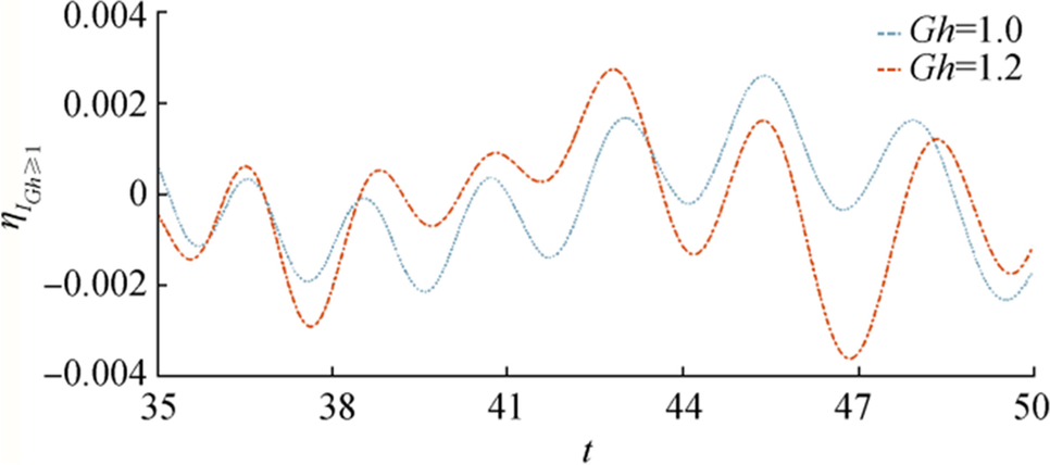
Figure 16 to Figure 19 show the behavior of $ {{{\boldsymbol{\eta}}}_{{\boldsymbol{I}}}}_{{\boldsymbol{G}}{\boldsymbol{h}}\ge 1} $ due to initial impulse for different parametric values. In Figure 16, $ {{{\boldsymbol{\eta}}}_{{\boldsymbol{I}}}}_{{\boldsymbol{G}}{\boldsymbol{h}}\ge 1} $ is plotted against $ {\boldsymbol{t}} $ for fixed $ {\boldsymbol{r}},{\boldsymbol{\epsilon}},{\boldsymbol{D}} $ and different values of porosity parameter. Amplitude of $ {{{\boldsymbol{\eta}}}_{{\boldsymbol{I}}}}_{{\boldsymbol{G}}{\boldsymbol{h}}\ge 1} $ increases as time increases and variation of $ {{{\boldsymbol{\eta}}}_{{\boldsymbol{I}}}}_{{\boldsymbol{G}}{\boldsymbol{h}}\ge 1} $ almost coincides for the two cases $ {\boldsymbol{G}}{\boldsymbol{h}}=1,\boldsymbol{ }1.2 $.
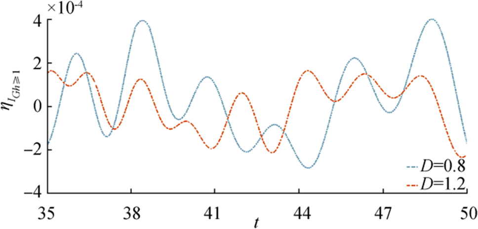
Wave motion due to initial impulse for fixed $ {\boldsymbol{r}},{\boldsymbol{\epsilon}},\boldsymbol{ }{\boldsymbol{G}}{\boldsymbol{h}} $ is shown in Figure 17. From this figure, it is observed that as $ {\boldsymbol{D}} $ increases amplitude of wave motion, it reduces considerably. Similar behavior observed in Figures 18 and 19, in which $ {{{\boldsymbol{\eta}}}_{{\boldsymbol{I}}}}_{{\boldsymbol{G}}{\boldsymbol{h}}\ge 1} $ plotted against $ {\boldsymbol{r}} $ for fixed $ {\boldsymbol{t}},{\boldsymbol{\epsilon}},{\boldsymbol{D}} $ and $ {\boldsymbol{r}},{\boldsymbol{\epsilon}},{\boldsymbol{G}}{\boldsymbol{h}} $, respectively.
5.3 Validation through comparison with previous results
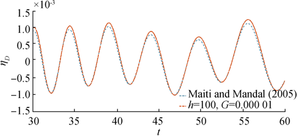
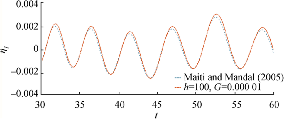
In this section, we compared our result with the existing result of Maiti and Mandal (2005), taking the depth of fluid region, $ {\boldsymbol{h}} $ is large and porosity parameter $ {\boldsymbol{G}} $ is quite small. In Figures 20 and 21, graphical behavior of free surface depression $ {\boldsymbol{\eta}} $ is shown in case of initial axially symmetric depression and impulse (taken as Dirac Delta function). In both, the figures dotted curve shows the nature of $ {\boldsymbol{\eta}} $ against $ {\boldsymbol{t}} $ for the existing result of Maiti and Mandal (2005) for fixed $ {\boldsymbol{r}}=60,\boldsymbol{ }\boldsymbol{ }{\boldsymbol{\epsilon}}=0.01,\boldsymbol{ }\boldsymbol{ }{\boldsymbol{D}}=0.5 $ and the thick curve shows behavior of $ {\boldsymbol{\eta}} $ for our result, against $ {\boldsymbol{t}} $ for fixed $ {\boldsymbol{r}}=60,\boldsymbol{ }{\boldsymbol{\epsilon}}=0.01,\boldsymbol{ }\boldsymbol{ }{\boldsymbol{D}}=0.5 $ and taking $ {\boldsymbol{h}}=50,\boldsymbol{ }\boldsymbol{ }{\boldsymbol{G}}=0.00001 $. In both figures, these two curves (dotted and thick lines) represent the nature of wave motion match quite well with each other.
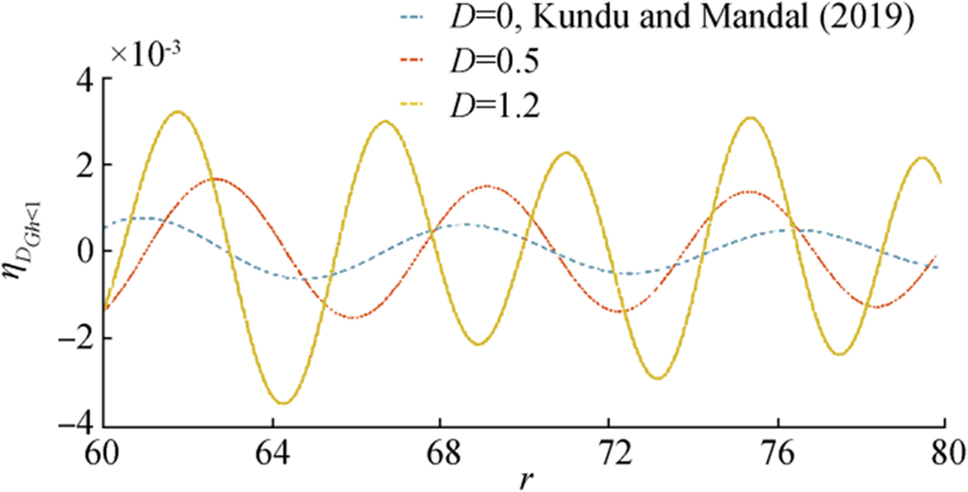
Here, we consider another comparison between the present result and Kundu and Mandal's (2019) result. Kundu and Mandal (2019) considered the generation problem by an initial axisymmetric surface disturbance in presence of porous bottom. In Figure 22 we have drawn both the results side by side, which shows the clear effect of ice cover on $ {\boldsymbol{\eta}} $ curve for initial depression. The curves are drawn for fixed values of $ {\boldsymbol{t}}=20,\boldsymbol{ }{\boldsymbol{\epsilon}}=0.01,\boldsymbol{ }{\boldsymbol{G}}{\boldsymbol{h}}=0.5. $ The dotted line represents Kundu and Mandal's (2019) data with no ice cover and the thick line shows the present result. The present result is drawn considering two different values of $ {\boldsymbol{D}}=0.5 $ and $ 1.2 $. From the figure, it is quite clear that the presence of ice cover shows more oscillation and amplitude in the wave depression curve.
For a clearer comparison, we have tabulated the present data and Maiti and Mandal (2005)'s data side by side in Table 1, for fixed $ {\boldsymbol{r}}=60,\boldsymbol{ }{\boldsymbol{\epsilon}}=0.01,\boldsymbol{ }{\boldsymbol{D}}=0.5. $
Table 1 Depression of ice cover for $ {\boldsymbol{r}}=60,\boldsymbol{ }{\boldsymbol{\epsilon}}=0.01,\boldsymbol{ }{\boldsymbol{D}}=0.5 $Items t Maiti and Mandal (2005) $\begin{aligned} &\text { Present result } \\ &\boldsymbol{h}=100, \boldsymbol{G}=0.00001 \end{aligned}$ Error $\text { Initial depression }\left(\boldsymbol{\eta}_{\boldsymbol{D}}\right)$ 30 0.00087 0.00096 0.00009 40 0.00051 0.00048 0.00003 50 0.00057 0.00066 0.00009 60 − 0.00059 − 0.00065 0.00006 $\text { Initial impulse }\left(\boldsymbol{\eta_{I}}\right)$ 30 − 0.00044 − 0.00041 0.00003 40 − 0.00055 − 0.00052 0.00003 50 − 0.00077 − 0.00075 0.00002 60 − 0.00016 − 0.00011 0.00005 Maiti and Mandal discussed the problem in infinitely deep water. In the present calculation, we consider very small values of $ {\boldsymbol{G}}=0.00001 $ and very large water depth $ {\boldsymbol{h}}=100 $. From the table, it is clear that the present result is matched with Maiti and Mandal's (2005) result up to 4 decimal places. This implies another check on the correctness of the results obtained here.
From these three figures and tabular values of ice-covered surface depression, it is observed that our result matches well with the existing result of the literature. This provides the desired check on the correctness of the method presented here.
5.4 Phase velocity, Group Velocity, and Wavelength
We consider the case of simple harmonic motion in time with angular frequency $ {\boldsymbol{\sigma}} $ to understand the behavior of surface waves in presence of ice-cover and porous bottom. The dispersion relation for surface wave in presence of porous bottom and ice-cover at the free surface can be written as
$$ \left(1+{\boldsymbol{D}}{{\boldsymbol{k}}}^{4}-{\boldsymbol{K}}{\boldsymbol{\epsilon}}\right){\boldsymbol{k}}\left(\frac{{\boldsymbol{k}}\boldsymbol{ }{t}{a}{n}{h}\boldsymbol{ }{\boldsymbol{k}}{\boldsymbol{h}}-{\boldsymbol{G}}}{{\boldsymbol{k}}-{\boldsymbol{G}}{t}{a}{n}{h}\boldsymbol{ }{\boldsymbol{k}}{\boldsymbol{h}}}\right)={\boldsymbol{K}} $$ (38) where $ {\boldsymbol{K}}={{\boldsymbol{\sigma}}}^{2} $. Neglecting $ {\boldsymbol{\epsilon}} $ in Eq. (36) the phase velocity $ {\boldsymbol{c}} $ and group velocity $ {{\boldsymbol{c}}}_{{\boldsymbol{g}}} $ are obtained as
$$ {\boldsymbol{c}}=\sqrt{\left({\boldsymbol{D}}{{\boldsymbol{k}}}^{3}+\frac{1}{{\boldsymbol{k}}}\right)\left(\frac{{\boldsymbol{k}}{t}{a}{n}{h}\boldsymbol{ }{\boldsymbol{k}}{\boldsymbol{h}}-{\boldsymbol{G}}}{{\boldsymbol{k}}-{\boldsymbol{G}}{t}{a}{n}{h}\boldsymbol{ }{\boldsymbol{k}}{\boldsymbol{h}}}\right)} $$ (39) and
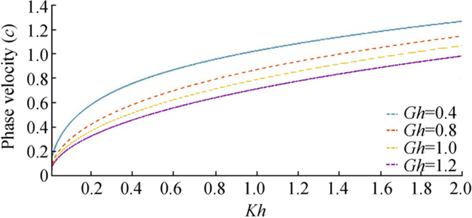
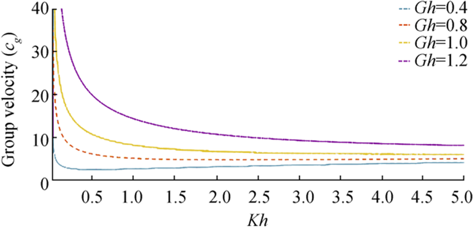
$$ {{\boldsymbol{c}}}_{{\boldsymbol{g}}}=\frac{{s}{e}{c}{{h}}^{2}{\boldsymbol{k}}{\boldsymbol{h}}}{4{\boldsymbol{\sigma}}{\left({\boldsymbol{k}}-{\boldsymbol{G}}{t}{a}{n}{h}\boldsymbol{ }{\boldsymbol{k}}{\boldsymbol{h}}\right)}^{2}}\left[2{\boldsymbol{k}}\left(1+{\boldsymbol{D}}{{\boldsymbol{k}}}^{4}\right)\left({\boldsymbol{G}}-\left({{\boldsymbol{G}}}^{2}+{{\boldsymbol{k}}}^{2}\right){\boldsymbol{h}}\right)+\left(1+5{{\boldsymbol{D}}{\boldsymbol{k}}}^{4}\right)\left(\left({{\boldsymbol{G}}}^{2}+{{\boldsymbol{k}}}^{2}\right){s}{i}{n}{h}\boldsymbol{ }2{\boldsymbol{k}}{\boldsymbol{h}}-2{\boldsymbol{G}}{\boldsymbol{k}}{c}{o}{s}{h}\boldsymbol{ }2{\boldsymbol{k}}{\boldsymbol{h}}\right)\right] $$ (40) Figures 23 and 24 demonstrate phase velocity $ ({\boldsymbol{c}}) $ against wave number, and Figures 25 and 26 demonstrate the variation of group velocity ($ {{\boldsymbol{c}}}_{{\boldsymbol{g}}} $) against wave number. Figures 23 and 25 show the variation of phase velocity and group velocity, respectively, for a fixed value of flexural rigidity coefficient $ {\boldsymbol{D}}=1.2 $ and taking different values of $ {\boldsymbol{G}}{\boldsymbol{h}}=0.4,\boldsymbol{ }0.8,\boldsymbol{ }\boldsymbol{ }{a}{n}{d}\boldsymbol{ }1.2 $. Increasing values of porosity parameter increase both $ {\boldsymbol{c}} $ and $ {{\boldsymbol{c}}}_{{\boldsymbol{g}}} $ and it is clearly seen from the figures that for each value of porosity parameter, $ {{\boldsymbol{c}}}_{{\boldsymbol{g}}}\boldsymbol{ } \gt {\boldsymbol{c}} $ with varying wave number.
From Figure 25, it can be seen that $ {{\boldsymbol{c}}}_{{\boldsymbol{g}}} $ attains its maximum value for a very small wave number and each $ {{\boldsymbol{c}}}_{{\boldsymbol{g}}} $ curve decreases with large values of wavenumber.
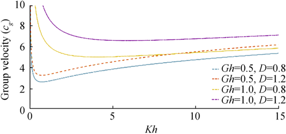
Figures 24 and 26 depict the phase velocity and group velocity, respectively, against wave number for fixed values of $ {\boldsymbol{G}}{\boldsymbol{h}}=0.5 $ and $ 1 $ and different values of flexural rigidity coefficient $ {\boldsymbol{D}}=0.8,\boldsymbol{ }1.2 $. It is seen that with increasing values of rigidity coefficient magnitude of phase velocity and group velocity both increase. Comparing Figures 24 and 26, it can be observed that with each fixed value of rigidity parameter always $ {{\boldsymbol{c}}}_{{\boldsymbol{g}}}\boldsymbol{ } \gt {\boldsymbol{c}} $. Figure 24 depicts that for small values of wave number; the phase velocity curves corresponding to different values of $ {\boldsymbol{D}} $ are shown nearly the same behavior whereas a more prominent increasing nature of the curves is shown for large wavenumbers. At the zero wave number, phase velocity attains minimum value, nearly zero; hence progressive wave does not propagate there.
From Figure 26, it is clear that varying porosity parameters $ {{\boldsymbol{c}}}_{{\boldsymbol{g}}} $ initially decrease. It has attained a minimum value for $ {\boldsymbol{K}}{\boldsymbol{h}} \lt 1 $ but with large values of wavenumber, it again increases.
6 Conclusions
In the present study, wave generation due to an initial axisymmetric disturbance at the surface of an ice-covered ocean with a porous bed is studied using Laplace and Hankel transform method under the assumption of linear water wave theory. The integral representation of the upper surface elevation is approximated by using the stationary phase method. The form of ice-covered surface depression is depicted graphically in a number of figures against time for some fixed distances from the shoreline and against the distances from the shoreline for some fixed values of time for two types of initial axially symmetric disturbances. The figures are drawn with either different values of the rigidity coefficient of the thin elastic ice sheet or different values of the porosity parameter of the sea bed. Here we consider the porosity parameter real. It is observed from the figures that as the flexural rigidity of the thin ice sheet increases, the plate can resist the generation of the surface wave so that the oscillatory nature of the wave reduced significantly. Further ocean waves generating in the ice field are observed to decrease in amplitude, and this observed reduction is preferably due to the presence of both ice sheet and bottom porosity. In the presence of a porous bed and ice cover, the phase velocity and group velocity of the gravity waves are depicted graphically in some figures for time-harmonic motion.
-
Table 1 Depression of ice cover for $ {\boldsymbol{r}}=60,\boldsymbol{ }{\boldsymbol{\epsilon}}=0.01,\boldsymbol{ }{\boldsymbol{D}}=0.5 $
Items t Maiti and Mandal (2005) $\begin{aligned} &\text { Present result } \\ &\boldsymbol{h}=100, \boldsymbol{G}=0.00001 \end{aligned}$ Error $\text { Initial depression }\left(\boldsymbol{\eta}_{\boldsymbol{D}}\right)$ 30 0.00087 0.00096 0.00009 40 0.00051 0.00048 0.00003 50 0.00057 0.00066 0.00009 60 − 0.00059 − 0.00065 0.00006 $\text { Initial impulse }\left(\boldsymbol{\eta_{I}}\right)$ 30 − 0.00044 − 0.00041 0.00003 40 − 0.00055 − 0.00052 0.00003 50 − 0.00077 − 0.00075 0.00002 60 − 0.00016 − 0.00011 0.00005 -
Banerjea S, Rakshit P, Maiti P (2011) On the waves generated due to a line source present in an ocean with an ice cover and a small bottom undulation. Fluid Dyn Res 43(2): 384–410. https://doi.org/10.1088/0169-5983/43/2/025506 Bhattacharjee J, Sahoo T (2008) Flexural gravity wave generation by initial disturbances in the presence of current. J Marine Sci Tech 13: 138–146. https://doi.org/10.1007/s00773-007-0269-2 Chung H, Fox C (2002) Calculation of wave-ice interaction using the Wiener-Hopf technique. New Zealand J Math 31(1): 1–18 Das L, Mohapatra S (2019) Effects of flexible bottom on radiation of water waves by a sphere submerged beneath an ice-cover. Meccanica 54: 985–999. https://doi.org/10.1007/s11012-019-00998-1 Fox C, Squire VA (1994) On the oblique reflexion and transmission of ocean waves at shore fast sea-ice. Phil Trans R Soc Lond, A 347;185–218. https://doi.org/10.1098/rsta.1994.0044. Gayen R, Islam N (2018) Effect of a floating elastic plate/membrane on the motion due to a ring source in water with porous bed Indian. J Pure Appl Math 49(2): 239–256. https://doi.org/10.1007/s13226-018-0266-7 Khuntia S, Mohapatra S (2020) Effects of ice-floe on surface wave interaction with an irregular flexible seabed. European J Mech 84: 357–366. https://doi.org/10.1016/j.euromechflu.2020.07.002 Kranzer HC, Keller JB (1959) Water waves produced by explosions. J of Appl Phys 30(3): 398–407. https://doi.org/10.1063/1.1735176 Kundu P, Mandal BN (2019) Generation of surface waves due to initial axisymmetric surface disturbance in water with a porous bottom. Int J of Appl Mech and Eng 24: 625–644. https://doi.org/10.2478/ijame-2019-0039 Lamb H (1945) Hydrodynamics. Dover, NewYork, pp 351–469 Maiti P, Mandal BN (2005) Water waves generated due to initial axisymmetric disturbances in water with an ice cover. Arch Appl Mech 74: 629–636. https://doi.org/10.1007/s00419-005-0384-7 Maiti P, Mandal BN (2014) Water wave scattering by an elastic plate floating in an ocean with a porous bed. Appl Ocean Res 47: 73–84. https://doi.org/10.1016/j.apor.2014.03.006 Mandal BN, Mukherjee S (1989) Water waves generated at an inertial surface by an axisymmetric initial surface disturbance. Int J Math Educ Sci Technol 20: 743–747. https://doi.org/10.1080/0020739890200512 Meylan MH, Squire VA (1996) Response of a circular ice floe to ocean waves. J Geophys Res 101: 8869–8884. https://doi.org/10.1029/95jc03706 Mohapatra S (2014) Scattering of surface waves by the edge of a small undulation on a porous bed in an ocean with ice-cover. J Marine Sci Appl 13: 167–172. https://doi.org/10.1007/s11804-014-1241-2 Mohapatra S, Bora SN (2009) Propagation of oblique waves over small bottom undulation in an ice-covered two-layer fluid. Geo Phy Astro Phy Fluid Dyn 103(5): 347–374. https://doi.org/10.1080/03091920903071077 Paul S, De S (2014) Wave scattering by porous bottom undulation in a two layered channel. J Marine Sci and Appl 13(4): 355–361. https://doi.org/10.1007/s11804-014-1276-4 Paul S, De S (2017) Wave scattering by uneven porous bottom in a three layered channel. J Marine Sci and Tech 22(3): 533–545. https://doi.org/10.1007/s00773-016-0430-x Rhodes-Robinson PF (1984) On the generation of water waves at an inertial surface. J Austral Math Soc Ser b 25: 366–383. https://doi.org/10.1017/S0334270000004124 Squire V (2007) Review of ocean waves and sea-ice revisited. Cold Regions Sci Tech 49(2): 110–133. https://doi.org/10.1016/j.coldregions.2007.04.007 Stoker JJ (1957) Water waves, the mathematical theory with applications. Pure and Applied Mathematics. Interscience Publishers, New York, Vol IV, 149–196. Sturova IV (2013) Unsteady three-dimensional sources in deep water with elastic cover and their application. J Fluid Mech 730:392–418. https://doi.org/10.1017/jfm.2013.303 Tsai C, Chen H, Lee F (2006) Wave transformation over submerged permeable breakwater on porous bottom. Ocean Eng 33:1623–1643. https://doi.org/10.1016/j.oceaneng.2005.09.006 Weitz M, Keller JB (1950) Reflection of water waves floating ice in water of finite depth. Comm Pure Appl Math 3:305–318. https://doi.org/10.1002/cpa.3160030306 Wen SL (1982) A note on water waves created by surface disturbances. Int J Sci and Math Edu 13:55–58. https://doi.org/10.1464/5211,0020-739X

