1   Introduction

In recent years, with the rapid development of the economy, the development scale of Chinese ports has been continuously expanding, and the traffic flow of ships in navigable waters has been increasing rapidly. At the same time, the traffic jam of the waterway also occurs frequently, and the navigation safety situation becomes increasingly severe. In order to prevent ship collision caused by maritime traffic congestion in busy waterways, more and more researches have been conducted, including navigable capacity estimation, maritime traffic analysis, ship behavior analysis and traffic complexity analysis (Liu et al., 2020; Ricci et al., 2020; Zhou et al., 2020). The prediction of vessel traffic volume provides a basic basis for the planning and design of waterways and navigation management of vessels. It enables the port department to scientifically and rationally plan the water area layout according to the changing rules of ship traffic flow, so as to improve the navigation efficiency of the waterway, which is of great significance for the improvement of navigation safety. Therefore, it is particularly important to design an algorithm that can accurately and effectively predict the flow of ships in the port to solve the problem of navigation safety.

At present, the main methods for forecasting ship traffic flow include regression analysis model, gray model (Guo et al. 2019), support vector machine, neural network, and combination model. The automatic identification system (AIS) data recording the ship's movement trajectory allows us to evaluate the operating efficiency of the ship when entering and leaving the port (Hongxiang et al. 2011). A time efficiency evaluation framework is proposed to evaluate the amount of time each ship spends in different internal areas. Watai et al. (2018) predicted the energy consumption of port ships and discusses strategies to reduce the energy consumption of port ships by using the proposed prediction model considering green ports. Pengfei et al. (2017) constructed the BP neural nets-Markov prediction model and modified the predicted value of the BP neural network by using the Markov prediction model to reduce the range of relative residual value and improve the accuracy of ship traffic flow prediction. Guo-Feng (2013) and Chan et al. (2018) introduced particle swarm optimization algorithm to optimize the model on the basis of the BP neural nets-Markov prediction model, which further improved the accuracy of the model prediction. But a major shortcoming of this research is that the BP neural network is not ideal for processing time-series data. Han et al. (2020) proposed an algorithm based on the cultural firefly algorithm to optimize the generalized regression neural network, which takes the weights between each layer in the network as the code to optimize and forecast the traffic flow of ships. The final experimental results show that the optimized algorithm has better generalization performance and higher result accuracy. The initial detection path of each UAV is obtained based on the minimum loop method. According to the time-invariant assumption commonly used in traditional traffic flow prediction, an intelligent particle swarm optimization algorithm is proposed by Chan et al. (2013). By combining the mechanism of PSO, neural network, and fuzzy inference system, a short-term traffic flow predictor is developed to adapt to the time-varying traffic flow. At present, BP neural network is widely used in traffic flow analysis (Qinghui et al. 2019). But BP neural network is based on the static feedforward network, which essentially transforms the dynamic complex time problem into the static spatial problem. But in fact, the ship's flow data is dynamic, and there is a certain relationship in time sequence (Xuantong et al. 2019). Therefore, the time factor and the process before reaching the temperature state will be ignored when the dynamic problem is converted to the static problem, which will directly affect the accuracy of the prediction results (Zhenguo and Shukui 2019; Ziwen 2020).

In this paper, on the basis of previous studies, the GRU-Markov prediction algorithm is designed. Due to the close relationship between port ship flow and time, compared with other algorithms, such as BP neural network, the method proposed in this paper to use GRU to predict ship flow has great advantages. Firstly, the GRU algorithm is used to preliminarily predict the port ship flow, and then the Markov algorithm is used to modify the neural network prediction results to further improve the accuracy of the algorithm prediction. The approximate algorithm flow is shown in Figure 1.

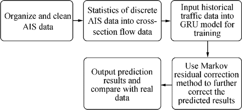Figure  1  Algorithm flowchart

Download: Full-Size Img

2   Data Analysis and Statistics Based on AIS

The original AIS data is discrete and has many redundant values. In fact, the ship's navigation behavior is mainly reflected in the change of the ship's navigation position with time. The dynamic information in the corresponding AIS information is longitude, latitude, speed, course, ROT, and update time. In order to distinguish the navigation behavior of different ships, maritime mobile service identity (MMSI) is added to the ship navigation behavior characterization data. Parts of the ship timing data screened out according to MMSI are shown in Table 1.

In this study, the number of ships passing through a certain section of the channel in a period of time is recorded to measure the traffic flow of ships. As shown in Figure 2, L1L2 is the observation section and ab is the line connecting the two AIS acquisition points of the ship. If the position relationship of the two lines is an intersection, it can be judged that the ship has passed the section of flow statistics.

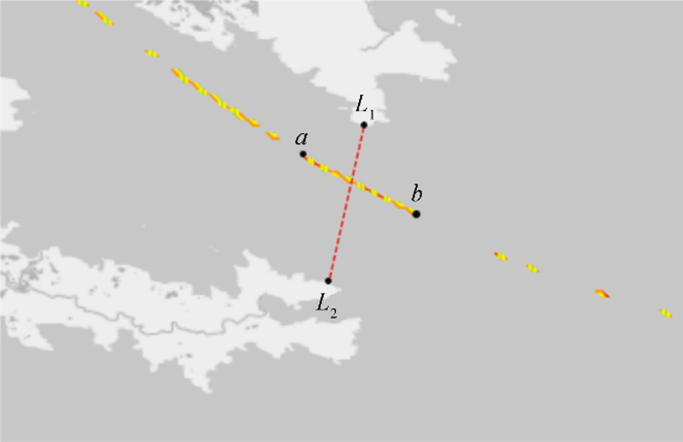Figure  2  Schematic diagram of navigation ship passing through observation section

Download: Full-Size Img

The position relationship of two-line segments includes coincidence, intersection, and separation. The ship can be included in the statistical range when the connecting line of two consecutive acquisition points intersects the line of flow statistics section. In this paper, the following algorithm is used to determine whether the two-line segments intersect.

1. Fast repulsion experiment: First, judge whether the projections of two-line segments coincide in X and Y coordinates. That is to judge whether the endpoint with a larger X in one-line segment is smaller than the endpoint with a smaller X in the other line segment. If so, it means that there must be no intersection point between the two-line segments. Similarly, judge y.

2. Straddle experiment: If two-line segments intersect, it means that they cross each other. If ab crosses L₁L₂, then a and b are located on both sides of the line where L₁ and L₂ are located. r_xy is used to represent the vector between x and y, then:

Similarly, the basis for judging L₁L₂ straddling ab is

The relationship between the straddling and fast rejection experiments is shown in Figure 3.

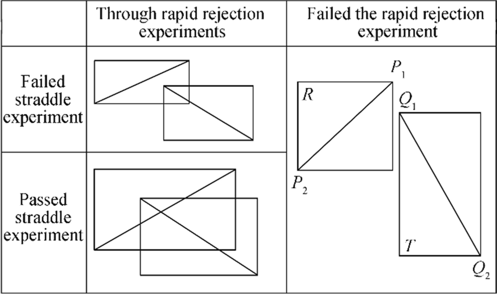Figure  3  Determination of intersection relation of line segments

Download: Full-Size Img

3   Foundation of Gated Recurrent Unit

3.1   Structure of Circular Neural Network

Neural network can be regarded as a black box that can fit any function. The traditional BP neural network fitting effect has been better, but it can only deal with each output separately. The former output is completely unrelated to the latter output, and the processing performance of sequence information is not good enough. Therefore, the structure of the recurrent neural network is proposed.

As shown in Figure 4, a simple circular neural network (RNN) consists of three parts: input layer x, hidden layer s, and output layer o. At any time t, the value of the network hidden layer $ {S}_{t} $ depends not only on the input $ {x}_{t} $ of the network at that time, but also on the output $ {S}_{t-1} $ of the hidden layer at the previous time, which shows that the RNN takes the timing information into account in the network structure, and the equation is as follows:

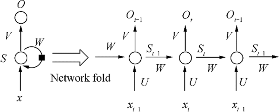Figure  4  RNN principle

Download: Full-Size Img

where f is the activation function of the hidden layer, and U and W represent the connection weight matrix from the input layer to hidden layer and between the hidden layer, respectively.

3.2   Gated Recurrent Unit

Because the common recurrent neural network has gradient disappearance and gradient explosion and cannot deal with long-term dependence and other problems, this paper adopts a special RNN; that is, the RNN unit in the network is replaced by gated recurrent unit (GRU), so as to solve the gradient disappearance and gradient explosion problems in standard RNN.

The input and output structures of GRU are the same as those of ordinary RNN, and their internal structure is slightly different from that of RNN. There are two gates in GRU, reset gate and update gate. Intuitively, the reset gate determines how to combine the new input information with the previous memory, while the update gate defines the amount of previous memory saved to the current time step. If the reset gate is set to 1 and the update gate is set to 0, a standard RNN model is obtained. The internal structure of GRU is shown in Figure 5.

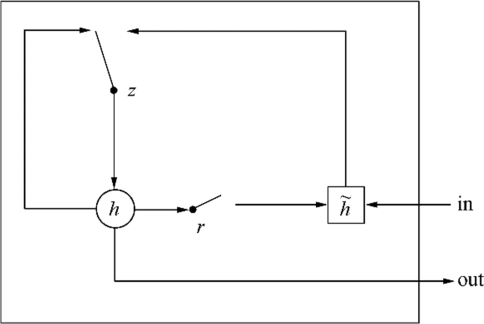Figure  5  GRU structure

Download: Full-Size Img

At time t, update gate $ {z}_{t} $ is calculated by the following equation:

where $ {x}_{t} $ is the input at the time t, $ \sigma $ is the sigmoid activation function, $ {h}_{t-1} $ is the information of the last moment, and W and U are weight matrices. The update gate adds the two parts of information and inputs it into the sigmoid function, so it compresses the activation result between 0 and 1.

The reset gate mainly determines how much past information needs to be forgotten. The calculation is as follows:

Its parameters are similar to the update gate, but the parameters and uses of a linear transformation are different.

In the use of the reset door, the new memory content will use the reset door to store the relevant information in the past, the calculation expression is as follows:

where $ \odot $ is the multiplication of the corresponding elements in the matrix on both sides.

Finally, calculating $ {h}_{t} $ determines the information to be passed to the next unit. This process is expressed as follows:

where $ {h}_{t} $ is the hidden state at the current time and the final output of GRU.

4   Modification of Initial Prediction Value Based on Markov Method

The navigation behavior of ships is an uncertain process, so the neural network structure trained by limited samples is usually not completely reliable. Because the state transition matrix has the ability to track the random fluctuation of variables, it can be used to correct the prediction results of neural networks, so as to improve the prediction accuracy of the prediction model. Markov chain can infer the possible state of a variable in the future based on the analysis of its current state and future change direction. However, the Markov method is not suitable for medium and long-term prediction. Therefore, this section applies it to the short-term prediction of ship flow to improve the prediction accuracy of the model.

According to the prediction value of the neural network, the relative error δ is calculated:

where $ {P}_{ex} $ is the neural network prediction of ship flow, and $ {P}_{n} $ is the actual flow of the ship.

When state $ {E}_{i} $ is transferred to state $ {E}_{j} $ after k times, the probability is as follows:

where $ {A}_{ij}^{(k)} $ is the number of transitions of sample state from $ {E}_{i} $ to state $ {E}_{j} $, and $ {A}_{i} $ is the total number of state occurrences.

The core of the Markov method is to determine the state probability transition matrix. In this paper, the state transition probability matrix $ {{\boldsymbol{P}}}^{(k)} $ is calculated according to the state of relative error:

where n is the number of states after classification.

The standard of state division is to take the upper and lower thresholds of the relative error δ of the predicted value of sample data as the range of state division.

Then, the initial state vector X (0) is determined according to the error data predicted by the ship flow prediction model, and the state transition result of step k is calculated by the state transition equation:

Finally, according to the relative error of Markov prediction, the corrected ship flow P is calculated:

where $ {}_{h} $, $ {}_{l} $ are the upper and lower thresholds of the error state interval.

5   Examples and Analysis

5.1   Data Analysis

The data studied in this paper comes from the AIS data of the Xiashimen water area in Zhoushan, Ningbo, in 2017. In the data, the water area of the ship sailing is 122.2° E, 29.8° N-122.35° E, 29.7° N. Different ships are distinguished by their MMSI codes. The navigation of the original ship in the water area is shown in Figure 6.

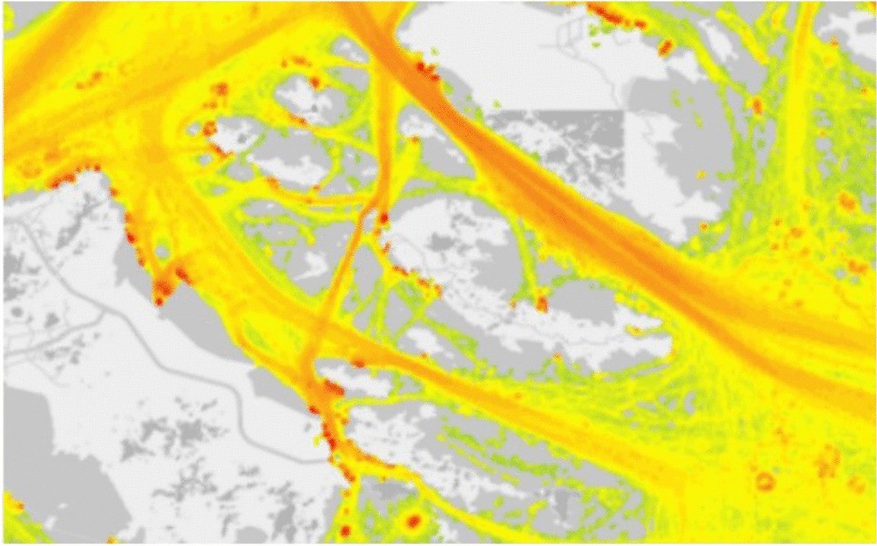Figure  6  Navigation of ships in waters

Download: Full-Size Img

The original data is preprocessed to roughly judge whether the ship's trajectory passes through the Xiazhimen water area. After the ships passing through the Xiazhimen gate are selected, the fast exclusion and straddle experiments are carried out on the tracks of each ship to determine the times and time points of the flow statistical Sects. (122.31° E29.75° N, 122.32° E 29.775° N). Part of the flow data after processing is shown in Table 2.

5.2   Construction of Neural Network Structure

In order to deeply mine the rules of the historical discharge data of the water area, this model takes the cross-section flow of five continuous time nodes as the input to build a time series ship flow prediction model (Hongxiang et al. 2011; He et al., 2019; Krizhevsky et al. 2017). The neural network model contains many hyperparameters, and the parameters that need to be adjusted are roughly divided into two categories. One is optimization parameters, such as learning rate and training algebra. One is the parameters of the model, such as the number of hidden layers and the number of neurons. The adjustment of hyperparameters has a great influence on the fitting effect of the model. For example, the learning rate affects the fitting speed of the model and the number of neurons and hidden layers affect the fitting effect of the model (Yanhong et al. 2016; Guo-Feng 2013; Ming-Wei et al. 2021). The model consists of one input node, five hidden layers (GRU layer, dropout layer, and dense layer) and one output node. The number of hidden layers and the number of neurons are determined based on experience. The input data length of the input node is n and the dimension is 1. After passing through five hidden layers, it is output at the output node, and the output is the ship flow of the next time node. The structures of the five hidden layers are as follows: the first GRU layer with 100 neurons. The second layer is the dropout layer with a probability of 0.2. The third layer is the GRU layer with 100 neurons. The fourth layer is the dropout layer with a probability of 0.2. The fifth layer is the dense layer with 1 neuron, which is used to connect the neurons in the upper layer to form one-dimensional output. The structure of the neural network is shown in Figure 7.

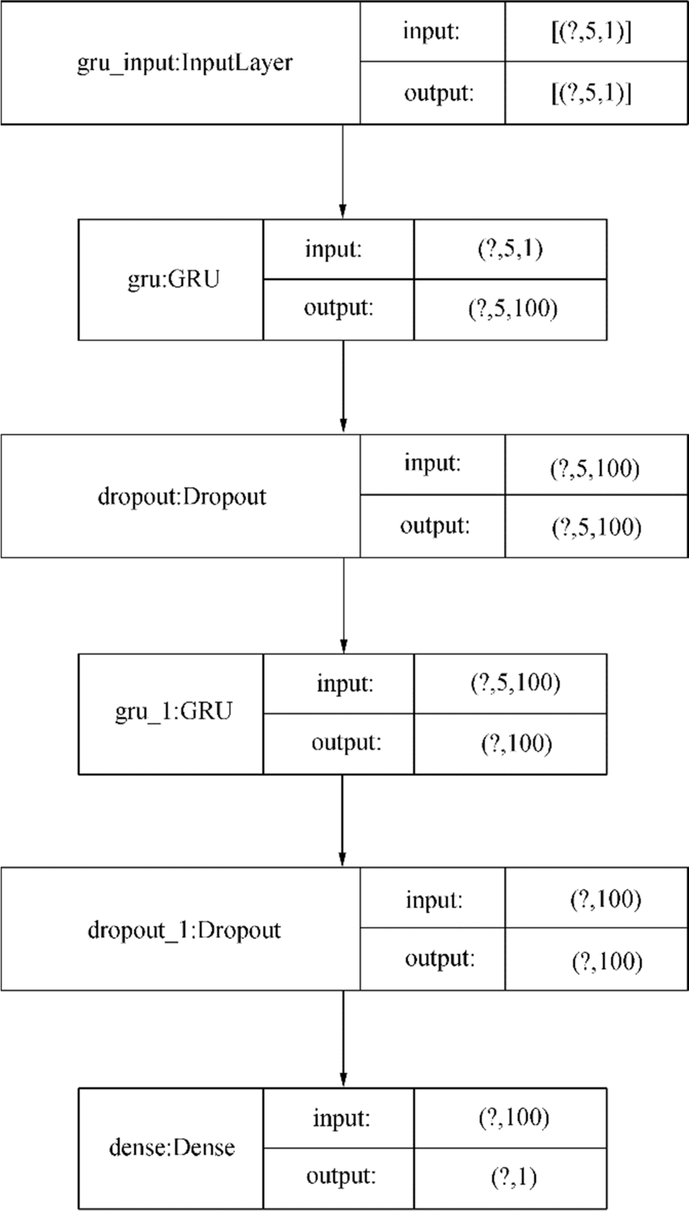Figure  7  Neural network structure

Download: Full-Size Img

Dropout layer was proposed in 2012 and applied to neural networks, mainly to prevent model overfitting. The direct function of dropout layer is to reduce the number of intermediate features, thus reducing redundancy and increasing the orthogonality of each feature in each layer. According to relevant experience, the probability of dropout is set to 0.2.

The learning of neural networks is a process of continuous error correction, that is, the final data calculated each time is compared with the actual data and the error is obtained, and then the weight is continuously adjusted until the error is reduced to an acceptable level. The loss function selected in this paper is the mean square error (MSE) function, which is one of the commonly used machine learning loss functions. It mainly measures the quality of the fitted data. The smaller the value, the closer it is to the actual value. The equation of mean square error function is as follows:

In the model optimization, an adaptive moment estimation (Adam) optimization algorithm is selected. Based on the original gradient descent algorithm, it tracks the exponential decay average of the past gradient to continuously optimize the model.

5.3   Input Data Processing

Because different indicators often have different dimensions and units, which will greatly affect the results of data analysis, therefore, in order to eliminate the dimensional impact between indicators, it is necessary to standardize the data. The standardization method selected in this paper is min-max normalization, which is a linear transformation of the original data, mapping all the data to 0-1. The equation is as follows:

where max is the maximum value of sample data and min is the minimum value of sample data.

6   Experimental Results

In this paper, the ship traffic flow data of 5 h before the flow section is used to predict the ship traffic flow of the sixth hour. For example, the ship traffic flow data from 0:00 on May 1, 2017, to 5:00 on May 1, 2017, is used as the input to predict the ship flow from 5:00 to 6:00 on May 1, 2017. The prediction results and errors of May 5 are shown in Figure 8 and Table 3. The table shows the error comparison between the predicted data and the actual value of the day. In Figure 8, the abscissa is each time point in a day, and the ordinate is the number of ships.

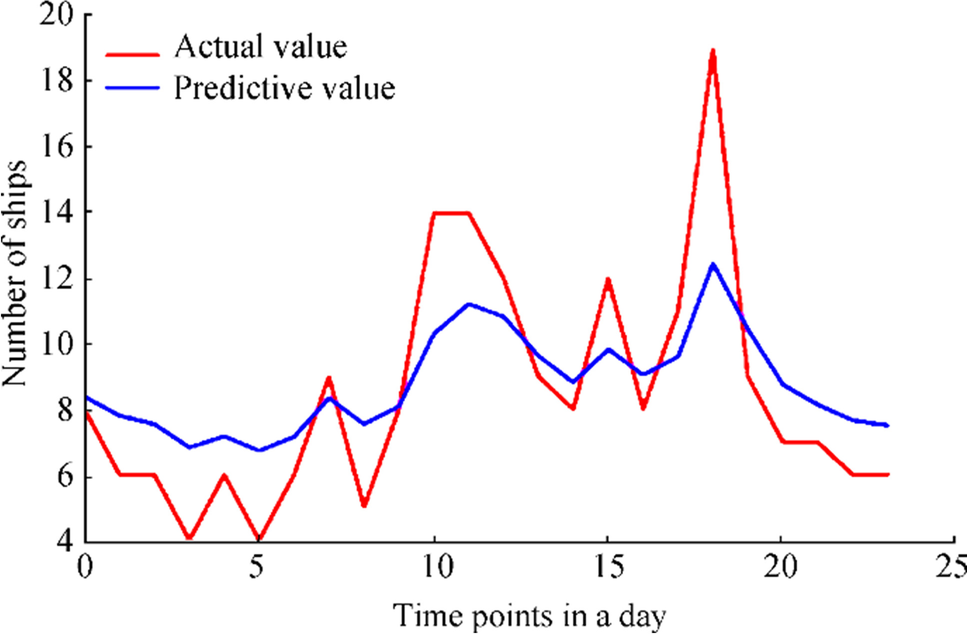Figure  8  Graph of GRU prediction results

Download: Full-Size Img

As can be seen from Figure 8, the GRU model can well fit the characteristics of less flow in the early morning of a day and the peak flow from noon to afternoon. However, due to the randomness of ship flow, when there is a small peak in a certain period of time (as shown in Figure 8, the flow of 18:00-19:00 is significantly higher than other periods), the effect of model fitting is not very accurate. Therefore, this paper uses the Markov method to correct the initial prediction value to make the predicted value closer to the real value.

6.1   Markov Residual Correction

In order to verify the correction effect of the Markov method on the initial prediction data of neural network, taking the prediction result of ship flow in May 2017 as an example, the relative error δ is obtained through calculation, and some data are shown in Table 4. The actual value and predicted value are arranged in time, and the state of relative error δ is determined by Table 4. In this paper, the predicted relative error is divided into four states according to the state division standard: [− 30%, − 15%], E₂ (− 15%, 0], E₃ (0, 15%], E₄ (15%, 30%], and based on this, the Markov state table is established, as shown in Table 5.

From Table 5, we can determine the Markov state transition matrix $ {{\boldsymbol{P}}}^{(1)} $:

Markov modified predicted value was shown in Figure 9. Taking the ship flow data of sequence 1 of the selected data as the initial state vector, that is, X (0) = (0, 0, 1, 0), then the state vector X (1) = X (0)$ {{\boldsymbol{P}}}^{(1)} $= (9/58, 7/29, 13/58, 11/29). Therefore, the probability that the prediction relative error δ of sequence 2 is in E₄ is the largest. According to the prediction results of the neural network, we can know that the predicted ship flow at sequence 2-time point is $ {p}_{1} $=7.5381. According to modified Eq. (12), the modified ship flow $ {p}_{\text{Markov}} $=5.8420 of the Markov chain can be calculated.

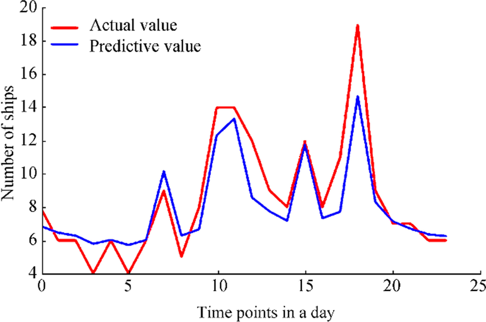Figure  9  Markov modified predicted value

Download: Full-Size Img

Given that the actual ship flow at sequence 2-time point is $ {p}_{2} $=6, the relative error δ = 25.63% before Markov correction is w, and the relative error after Markov correction is δ = − 2.66%. According to the same method, the ship flow correction value of each subsequent sequence point can be calculated.

6.2   Comparative Experiment of Prediction Model

In order to verify the advantages of the proposed GRU-Markov prediction model in prediction accuracy, the prediction results of the proposed algorithm are compared with those of other algorithms. The comparison algorithms are GRU algorithm without Markov optimization, SVM, and BP neural network. The results of the comparison are shown in Table 6.

The results show that, considering the relationship between ship flow and time series, the prediction results of the GRU neural network are generally closer to the real value than support vector machine and BP neural network, and the error is further reduced after Markov correction. Therefore, the performance of GRU-Markov is better than other algorithms.

7   Conclusion

Based on the research of ship flow prediction method, combined with the characteristics of AIS data information, the AIS data are sorted and counted by using fast exclusion and straddle experiment. The discrete AIS data are counted into traffic data arranged in time series. Considering the influence of time series type data before and after, this paper proposes to apply the GRU algorithm to ship flow prediction. A neural network prediction model based on GRU-Markov is constructed. The ship flow data of five consecutive time points are used as input to predict the ship flow data of the next time point. GRU is used to make basic predictions, and then the Markov method is applied to modify the initial prediction value. The proposed algorithm is verified by a large number of AIS data near Xiazhimen, Zhoushan, Ningbo, and compared with the traditional prediction algorithm SVM and BP neural network, it proves that the algorithm in this paper has great advantages in prediction accuracy and algorithm time-consuming. However, due to the characteristics of a large amount of historical data required for the training of the neural network itself, the algorithm in this paper also has certain limitations. For example, it may not be applicable under the conditions of insufficient historical data, etc. Through the above work, it is proved that the GRU-Markov model is practical and effective in the prediction of ship flow, and also provides a new theoretical basis for the prediction of ship track in the future.