1   Introduction

As one of the main underwater acoustic detection tools, the sonobuoy has great importance in underwater object localization and ambient noise record (Barlow et al. 2018; Tan et al. 2011; Tollefsen and Sagen 2013, 2014). However, the flow noise caused by vertical motion2.2 of the sonobuoy limits its working performance. Since the surface buoy of the sonobuoy will move up and down with the sea waves, and this forced movement can be transmitted to underwater hydrophones by the cable, which causes relative movement between the hydrophone and the surrounding seawater. As a result, it generates pressure fluctuations on the hydrophone surface, which can be sensed by the hydrophone (Auvinen et al. 2019). In some cases, the noise level of the flow noise is much greater than the noise level of ambient noise, which reduces the signal-to-noise ratio (SNR) of the sonobuoy (Holler 2014; Willis et al. 2013). Moreover, according to the research of McEachern (1995), the flow noise can be generated even at very small stream velocity. As the detected target grows quieter, reducing the flow noise of sonobuoy is of great significance for improving working the performance of the sonobuoy.

The flow noise of the sonobuoy studied in this paper is generated from the pressure fluctuations which are caused by the sinusoidal vertical motion of the hydrophone. Therefore, it should to decouple the underwater hydrophone of the sonobuoy from the large vertical motions of the buoy on the sea surface. Kebe (1981) studied the self-noise of a suspended hydrophone on a moored sonobuoy. Some design criteria were given, and an equation for calculating the optimal length of the expandable rubber band was discussed in particular. Additionally, Gobat and Grosenbaugh (1997) detailed efforts to reduce the flow noise received by hydrophones on a surface suspended sonobuoy by combining the analysis of experimental data. The relationships between flow noise and acceleration of the hydrophone were discussed. The structure of the sonobuoy was improved, including replacing the array and the surface buoy with a single flow-shield hydrophone and a spar buoy, respectively. Chapman (2008) studied the sinusoidal vertical motion of the sonobuoy suspension by experiment. A low-pass mechanical filter comprising a bungee cord and a damper disk was employed to isolate the acoustic sensor from the large vertical motion of the buoy on the ocean surface. Huang et al. (2018) studied the flow noise of hydrophone caused by vertical heave of sonobuoy with mathematical and simulation calculations. They found that choosing bungee cords with appropriate elastic coefficients can effectively suppress the heave thus reduce the flow noise of sonobuoy. Additionally, Guan et al. (2020) also studied the sonobuoy suspension system composed of bungee cord and damping disk and established a mathematical model considering its added mass and non-constant drag coefficient.

Besides, the suppression effects of the suspension system on flow noise also need to be verified. The flow noise can be obtained by experiment and numerical calculation. Numerical calculation has the advantage of avoiding interference from other noise signals compared with experimental measurement. However, in those researches mentioned above, the flow noise of the sonobuoy was almost obtained by experiment. Numerical studies of the flow noise were started with Lighthill's acoustic analogy theory (Lighthill 1952, 1954). In recent year, the Ffowcs Williams-Hawkings (FW-H) equation (Ffowcs Williams and Hawkings 1969 which was developed from Lighthill equation has been used for the prediction of the underwater flow noise; e.g., Kellett et al. (2013), Ozden et al. (2016), Huang et al. (2019) and Khalid et al. (2019) used the CFD-based unsteady fluid field calculation approach, coupled with the FW-H equation for noise prediction. In this study, a hybrid numerical method was adopted to calculate the flow noise of the sonobuoy under time-varying stream velocity.

In this paper, a suspension system consisting of an elastic suspension cable and isolation mass was studied in details. The suspension system allows the surface buoy to follow the large vertical motions of the sea surface while leaving the sensitive hydrophone at the lower end relatively undisturbed, thereby reducing the flow noise caused by the vertical motion of hydrophone. In order to analyze the vertical motion of the optimized sonobuoy under different conditions, a theoretical motion model of the sonobuoy was given. The suppression laws of the suspension cable elastic constant, underwater part mass of the sonobuoy and sea wave period on hydrophone vertical motions were given. Combining the theoretical model of motion, a numerical calculation method based on CFD and FW-H was adopted to compute the flow noise of the sonobuoy, which can be used to evaluate the effect of suspension system on reducing flow noise. The paper is arranged as follows: Section II gives a theoretical vibration model based on sonobuoy and obtains the velocity responses under different parameters. Section III introduces the mathematical model for calculating flow noise. Section IV presents the simulation results of the velocity responses and the flow noise under different conditions and Sec. V summarizes the conclusions.

2   Theoretical Model

2.1   Differential Equation of Vertical Motion

This study focuses on reducing the flow noise caused by the sinusoidal vertical motion of sonobuoy. As the relative movement between the hydrophone and the seawater is caused by the sea waves, therefore, an elastic suspension cable and isolation mass were added to the sonobuoy to decouple the vertical motion of the buoy at the sea surface from the underwater hydrophones. Figure 1 depicts the structure diagram of the sonobuoy with a suspension system. The elastic suspension cable 3 is added between the surface buoy 1 and the cable 4, and the underwater part below the suspension cable includes cable 4, hydrophone 5, and counterweight 6. Sonobuoy can be divided into two parts: the surface part and the underwater part. The elastic suspension cable plays a damper between the two parts. The underwater part can be seen as a forced vibration system when the sonobuoy drifts in the sea surface. After analyzing the forces acting on the underwater part, we found that there are three kinds of force, i.e., an external force from the surface buoy which caused by the sea wave, the total negative buoyancy, and drag force.

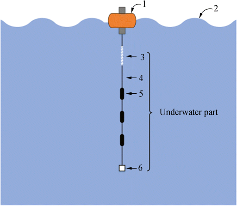Figure  1  Diagrammatic sketch of sonobuoy with a suspension system

Download: Full-Size Img

In order to analyze the vertical motion of the sonobuoy underwater part, a differential equation of motion of the underwater part was established, as shown in the following equation:

where

m is the total mass of the underwater part of the sonobuoy. $ \ddot{y} $ is the vertical motion acceleration, it equals d²y / dt², and y is the displacement of the underwater part. k is the elastic constant of the elastic rope. Here, Y represents the external excitation; L is the total length of the cable and the elastic suspension cable in a natural stretch state, d is the wave height of the sea wave, ω is the angular frequency of the surface wave and it equals 2π / T. T is the wave period. ΔG is the total negative buoyancy of the underwater part, and it equals to gravity minus its buoyancy. F is drag force. C is the drag coefficient, A is cross-sectional area of the sonobuoy, and ρ is the density of seawater.$ \dot{y} $ is the vertical motion velocity, it equals dy/dt. In this study, the positive velocity represents that the sonobuoy is moving upward.

The differential equation of motion can be solved using the fourth order Runge-Kutta algorithm, shown as follows:

which has the accumulative error in order of O(h⁴), and h is calculation step. The implementation of the theoretical model is described in Algorithm 1

2.2   Velocity Response Simulation

In this subsection, the vertical motion velocity responses of the sonobuoy underwater part under different sea states were analyzed in details. Table 1 (Sea state table of wave and wind levels 2020) lists the average height and average period of sea surface waves under different sea states. As the sea state above level 5 is already quite bad, in this study, only sea states below level 5 are discussed.

It should be noted that the waveforms corresponding to different sea states are simplified into sine waves in this study. They are taken as the external excitations of the sonobuoy differential equation of motion. The fluid velocity is an important factor for flow noise. Therefore, in this section, a velocity transmission rate T_r is defined, which is used to evaluate the effect of the suspension system on suppressing the vertical motion caused by the waves, as shown below:

where v_max is the maximum response velocity of the hydrophone and V_max is the maximum motion velocity of the surface buoy caused by the sea wave. The smaller T_r means the oscillation amplitude of the hydrophone caused by the wave under the same sea state is smaller.

There is a maximum motion velocity V_max for the surface buoy at each sea state. Besides, we can obtain a series maximum response velocity v_max of the hydrophone under different elastic constant k with Algorithm 1 when the mass m of sonobuoy underwater part remains the same. Similarly, a series maximum response velocity v_max of the hydrophone under different mass m can be obtained by Algorithm 1 when the elastic constant k remains the same. Moreover, there is a maximum response velocity v_max of the hydrophone corresponding to different sea state when the elastic constant k and mass m keep unchanged. Then, we can obtain the relationships between T_r and k, m, and sea state by Eq. (5), respectively.

Figure 2 depicts the relationships between T_r and k under different sea states. It shows that in each sea state, the velocity transmission rate decreases with the decreasing elastic constant of the elastic suspension cable. Figure 3 depicts the relationships between T_r and m under different sea states. It is indicated that in each sea state, the velocity transmission rate decreases with increasing mass. Figure 4 shows the relationships between T_r and sea state. Here, m = 20 kg and k = 5 N/m. The results show that under the same condition, the velocity transmission rate gradually increases, while the sea state becomes worse. This is because the wave period increases when the sea state becomes worse.

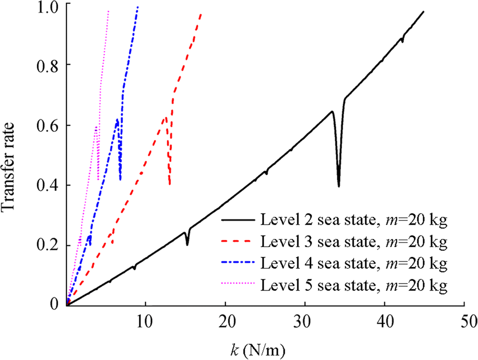Figure  2  Curve of T_r with k under different sea states

Download: Full-Size Img

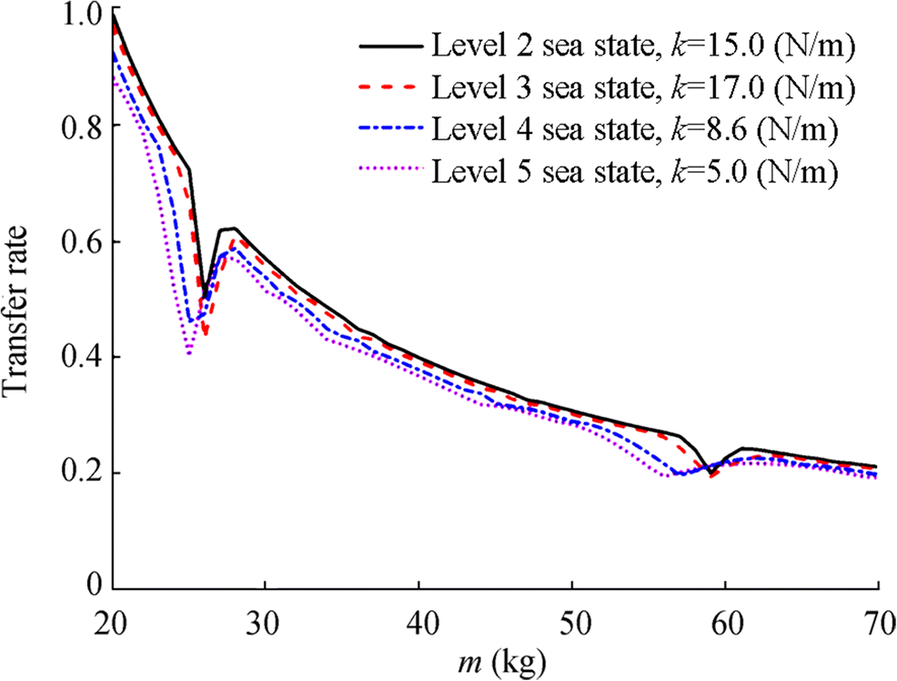Figure  3  Curve of T_r with m under different sea states

Download: Full-Size Img

Figure  4  Curve of T_r with sea state

Download: Full-Size Img

Table 2 lists the value ranges of the elastic constant at different sea states when the transmission rate is less than or equals to 1 and the mass is 20 kg.

Table 3 lists the value ranges of the mass at different sea states when the transmission rate is less than or equals to 1 and the elastic constant is 20 N/m.

By analyzing the data in Tables 2 and 3, it can be found that there is a relation between the wave angular frequency ω and the natural frequency ω_n. Among them, ω_n is the natural frequency of the sonobuoy, and ω_n = (k / m)^0.5. When T_r is equal to 1, the specific value of ω_n and ω approximately is equal to 0.578. The relationship between ω_n and ω is shown in Fig. 5. The pink area below the curve of ω_n = 0.578ω means that T_r is less than or equal to 1 under those conditions.

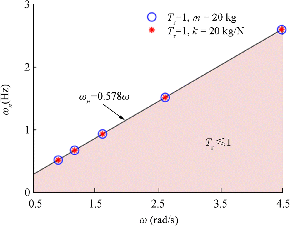Figure  5  The range of the ω_n in different sea states when T_r is less than or equal to 1

Download: Full-Size Img

Consequently, through the analysis above, it can be concluded that T_r is related to the mass of the sonobuoy underwater part, the elastic constant of the elastic rope and the external excitation period, i.e., T_r ∝ (ω_n/ω).

3   Flow Noise Calculation Method

Flow noise predictions based on CFD and FW-H will be investigated in two steps, first solving the flow field, followed by the acoustic computations.

3.1   Flow Field Equations

According to the law of mass conservation and momentum conservation, the Navier-Stokes (NS) (Huang et al. 2019) equations of three-dimensional incompressible viscous fluids can be written as

where f_i is an external force and (x_i, x_j) denotes the particle coordinates and it is the function on t. u_i and $ {u}_j^{\prime } $ are the average velocity and velocity fluctuation of the fluid, separately, i, j = 1, 2, 3, ρ is the density of the fluid, p is the average pressure, and υ is the kinematical viscosity coefficient. $ \overline{u_i^{\prime }{u}_j^{\prime }} $ is the Reynolds stress.

In this study, the renormalization group (RNG) k-ε two-equation turbulence models were used to calculate the flow field (Yakhot et al. 1992; Li et al. 2011; Tahmasebi et al. 2020). The RNG model has an additional term in its ε equation that significantly improves the accuracy of rapidly strained flows. Moreover, the effect of swirl on turbulence is included in the RNG model, enhancing the accuracy for swirling flows. The RNG theory provides an analytical formula for turbulent Prandtl number but not a constant. This improvement achieves good results in the simulation accuracy and the range of application. Besides, it has a better performance for the calculation of complex shear flow in the transition region. The RNG k-ε two-equation turbulent model used in this paper is given by

where C_k is production rate of turbulent kinetic energy, and σ_k, σ_ε, C_1ε and C_2ε are constants of the model.

3.2   Acoustic Field Equations

The Lighthill acoustic analogy theory was derived from the Navier-Stokes equation, and the generalized Lighthill equation (Lighthill 1952, 1954) in acoustic analogy theory was used to calculate the noise field. Its wave density equation is in the form of

whereρ^′is the density change by fluid disturbance, andρ^′ = ρ − ρ₀, ρ denotes the fluid density with the disturbance and ρ₀ denotes the fluid density without the disturbance. c₀ is the sound speed in the isentropic fluid. T_ij is the Lighthill stress tensor, which is defined as (Kim and Yoon 2020)

where p^′ = p − p₀, and p and p₀ denote the pressure of the fluid with and without the disturbance, respectively; τ_ij denotes the viscous stress, and δ_ij is the Kronecker symbol.

In this paper, we use the FW-H equation (Ffowcs Williams and Hawkings 1969) which is developed from the Lighthill's equation to simulated the flow noise,

in whichvp^′is the sound pressure of the far field, δ(f) is the Dirac delta function, and f is the wall function; H(f) is Heaviside function; and n_j is the unit normal vector pointing from the periphery of the solid to the flow field. u_i and is the fluid velocity in the x_i direction; u_n and v_n denote the fluid velocity and surface velocity components normal to the surface. P_ij is the compressive stress tensor, which is defined as below:

3.3   Validation of Simulated Flow Noise

The simulated flow noise of the hydrophone under a constant stream velocity was given, which has been verified by the experimental data. It should be noted that the experiment data were obtained from a submerged buoy rather than sonobuoy. Due to the lack of the flow noise experimental data of sonobuoy, the experimental data of flow noise received by the submerged buoy were selected to verify the simulated flow noise calculated by the hybrid numerical computation method in this study.

The following figures show the noise data which was measured by a submerged buoy in a deep-water experiment in the South China Sea. There is flow noise generated on the hydrophone during the descent of the submerged buoy. The noise data were sampled continuously at 20 Hz. The descent velocity of the submerged buoy can be computed by the depth sensor. The depth change of a hydrophone on the submerged buoy is shown in Fig. 6. It shows that the submerged buoy will descend at an approximately constant speed before completely stabilizing on the bottom of the sea. The blue line in Fig. 7 depicts the noise level of the noise data recorded by a hydrophone when the submerged buoy was stationary. The red line represents the noise level of the noise data received by the hydrophone when the submerged buoy was descending at a speed about of 1 m/s. In this study, the reference sound pressure for the noise level calculation is 10^-6 Pa. The result shows that the noise level of the generated flow noise is higher than that of ambient noise. Thereby, it will reduce the SNR of the sonobuoy.

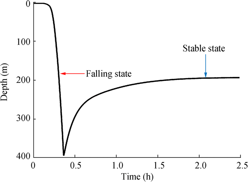Figure  6  Depth time series of hydrophone during descent process

Download: Full-Size Img

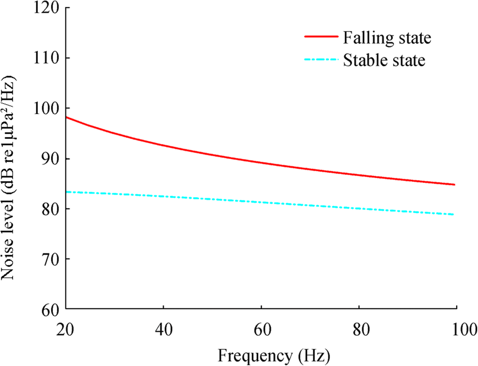Figure  7  The noise level of the data measured by experiments

Download: Full-Size Img

Next, we simulated the flow noise generated on the hydrophone of the submerged buoy during the descent with the numerical method. The relative movement between the hydrophone and the seawater can be seen as the seawater flowing past the stationary hydrophone at a certain stream velocity. The three-dimensional hydrophone model used for calculating the flow noise is shown in Fig. 8.

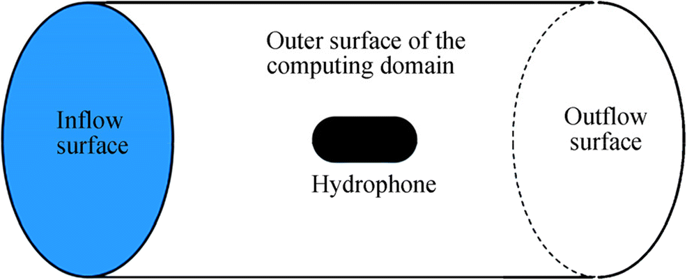Figure  8  The Computing Domain Used in CFD

Download: Full-Size Img

Flow noise calculation process:

(1) Establishing the model. The model was established regarding actual size of the hydrophone on the submerged buoy. The size ratio is 1:1. The maximum circumference and length of the hydrophone are 0.12 m and 0.10 m, respectively. The three-dimensional calculation domain used in CFD is a cylinder-topology, as shown in Fig. 8.

(2) Meshing the grid. In the calculation of CFD, the grid was chosen as body grid, which was created by commercial software ANSYS ICEM here. For the body grid, the non-dimensional spacing wall y⁺ was set as 40, and the total number of the grid for the computational domain is about 0.85 million according to the y⁺.

(3) Flow field calculation. The flow field was calculated with the FLUENT software. The flow field calculation boundary conditions are shown in Table 4. The RNG k-ε two-equation turbulent models were chosen in the flow field calculation. The finite volume method (FVW) was used to discrete the governing equations. The time step was set to be 10^-3 s, the stream velocity of the inflow surface was set to be 1 m/s, and the liquid density is 1024 kg/m³.

(4) Acoustic field calculation. The acoustic response of the flow field data was calculated with the FW-H integration approach. The sound speed is 1500 m/s.

The performance of the numerical calculation method is verified by the experiment data and empirical formula. Figure 9 shows the noise levels of flow noise obtained by numerical simulation and experiment at a stream velocity of 1 m/s. It depicts that the simulation result is in good agreement with that of the experimental data.

Figure  9  The noise level of flow noise at a stream velocity of 1 m/s

Download: Full-Size Img

Besides, based on the Lighthill equation, Lauchle (1977) derived the relationship between the noise power G and free-stream velocity v by the method of dimensional analysis. The relationship is given by

In this paper, three sets flow noise under time varying incoming stream velocity were calculated, as shown in Figure 10. The maximum values of the three sets stream velocity are 0.52, 0.98, and 1.53 m/s, respectively. From Fig. 10, we can found that the noise levels at same frequency are proportional to the fifth power of stream velocities, which is consistent with the conclusion presented by Lauchle.

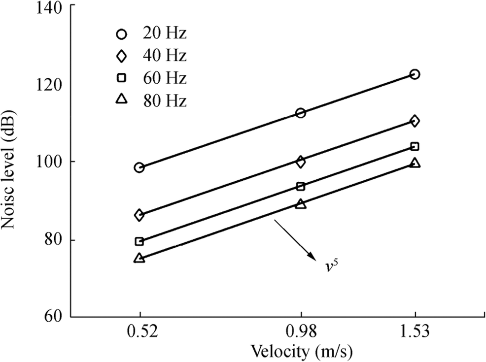Figure  10  Noise level of flow noise at different inflow velocities by simulation

Download: Full-Size Img

4   Flow Noise Numerical Simulation

A numerical method used for computing the flow noise of the sonobuoy is presented. The relative motion between the hydrophone and the seawater can be seen as the seawater flowing past the stationary hydrophone. The response velocities of the hydrophone under different conditions are obtained by solving the differential equation of motion. In this study, those response velocities are taken as the set value for the inflow surface by the User-Defined Function (UDF) to simulate the flow noise caused by the vertical motion of the hydrophone. The calculation process and boundary conditions are the same as those used in Sec. 3.3.

4.1   Different Elastic Coefficients

Figure 11 shows the incentive velocity under level 4 sea state and the response velocities of the hydrophone under different elastic constants. The incentive velocity is the vertical motion velocity of the surface buoy. When there is no elastic suspension cable on the sonobuoy, the response velocity of the hydrophone can be approximately replaced by the excitation velocity. The results show that the amplitude of these response velocities decreases with decreasing elastic constant.

Figure  11  The excitation velocity of a level 4 sea state and corresponding response velocity under different elastic constants (m = 20 kg)

Download: Full-Size Img

Figure 12 shows the pressure fluctuations on the wall of hydrophones under different incoming stream velocities, which were calculated by CFD. Figure12 (a) shows the pressure fluctuation calculated by using the excitation velocity under the level 4 sea state as the inflow boundary condition. Figures 12(b)-12(d) show the wall pressure fluctuations on the hydrophone calculated by using the response velocities as the inflow boundary conditions, where the response velocities were obtained when the elastic constants equal 7, 4, and 1 N/m, respectively. Here, the sea state is level 4 and the mass m = 20 kg.

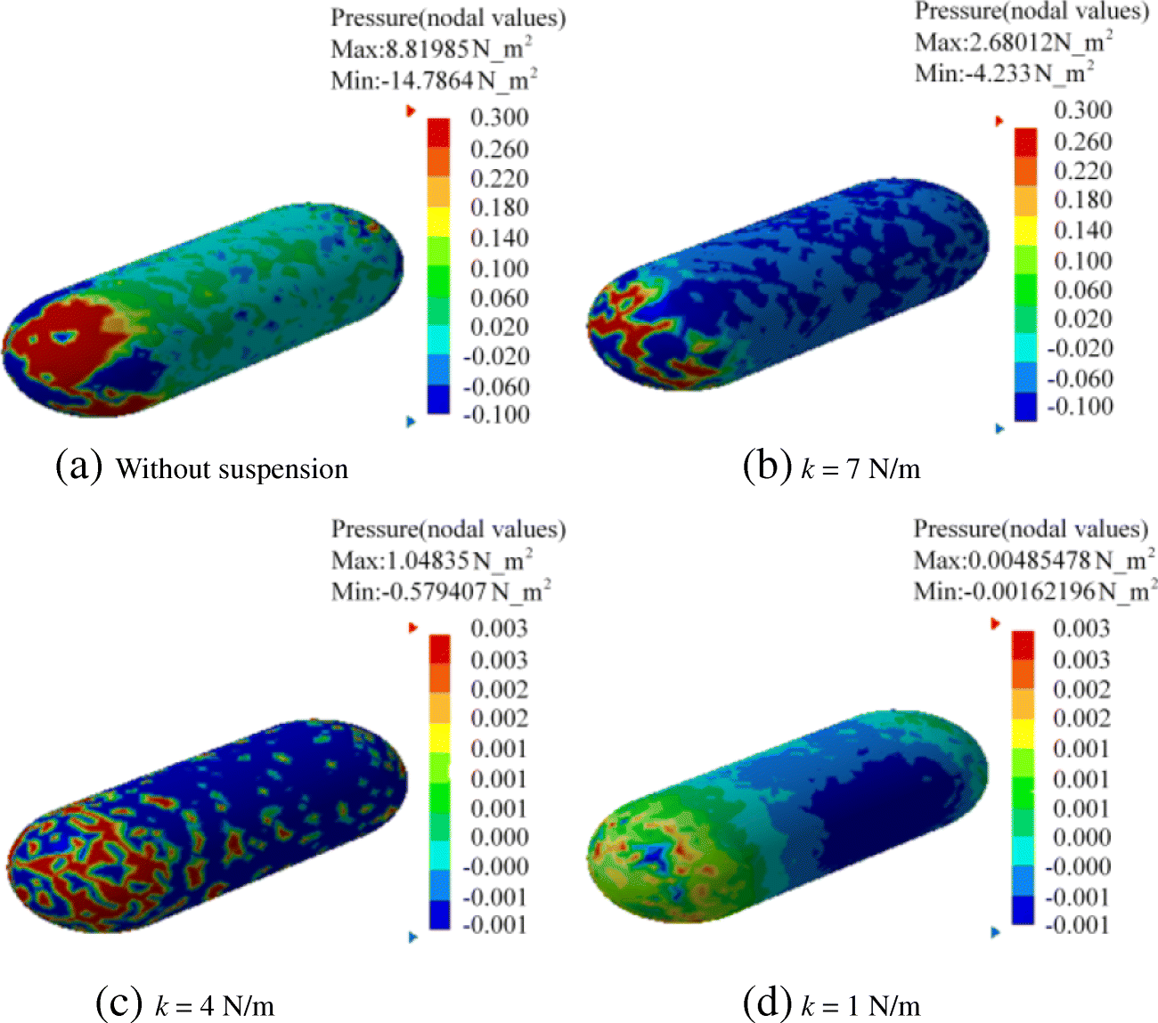Figure  12  The pressure fluctuation on the wall of hydrophone under different elastic constants (20 Hz)

Download: Full-Size Img

(a) Without suspension (b) k = 7 N/m

(c) k = 4 N/m (d) k = 1 N/m

It is indicated that the pressure fluctuations on the surface of the hydrophone gradually decrease with decreasing elastic constant of the elastic suspension cable. The pressure fluctuations shown in Fig. 12 were taken as the flow noise source and then computed their acoustic responses by the FW-H equation. The results are shown in Fig. 13. It is indicated that the noise level of the flow noise decreases with the decreasing elastic constant when the mass of the underwater part and the external excitation keep unchanged.

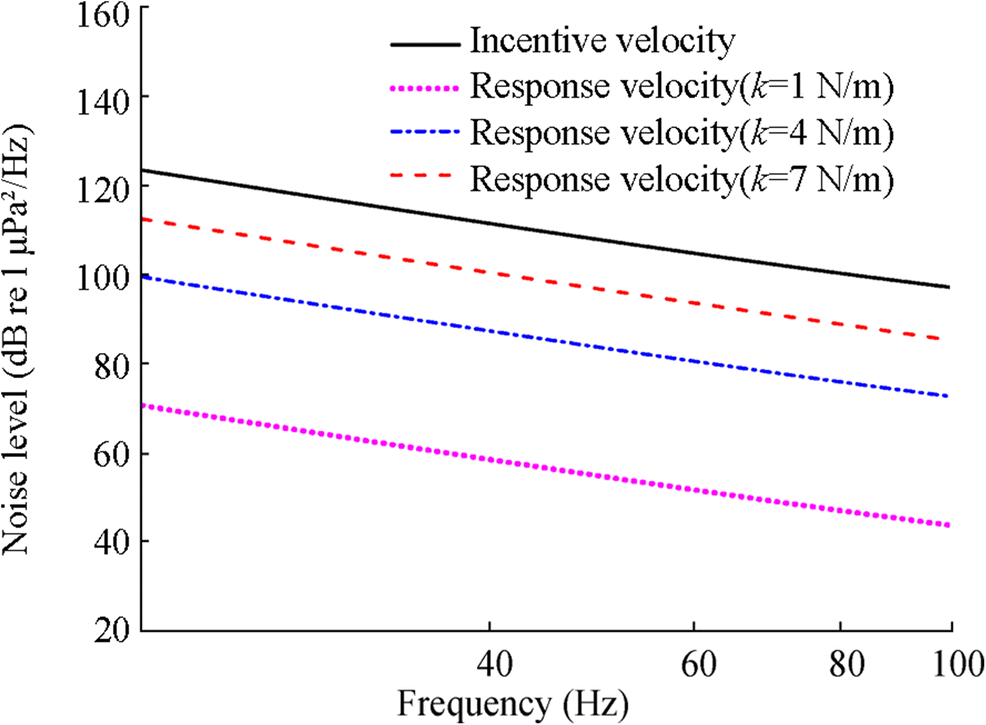Figure  13  The noise level of flow noise under different elastic constants

Download: Full-Size Img

4.2   Different Masses

Figure 14 shows the incentive velocity under the level 4 sea state and the response velocities of the hydrophone under different masses. The results show that when the elastic constant and the external excitation keep unchanged, the amplitude of the response velocity becomes smaller with the increasing mass.

Figure  14  The excitation velocity of level 4 sea state and corresponding response velocities under different masses (k = 8 N/m)

Download: Full-Size Img

Figures 15(a)-(c) depict the wall pressure fluctuations on the hydrophones calculated by using the response velocities as the incoming stream boundary conditions, where the response velocities were obtained when the mass is 20, 30, and 40 kg, respectively. The response velocities in the aforementioned three cases were calculated when the sea state is 4 level and k is 8 N/m.

(a) m = 20 kg

(b) m = 30 kg

(c) m = 40 kg

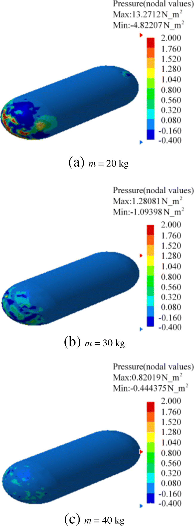Figure  15  The pressure fluctuation on the wall of hydrophone under different masses (20 Hz)

Download: Full-Size Img

Figure 15 shows that the wall pressure fluctuations on the surface on the hydrophones gradually decrease with increasing mass. The pressure fluctuations shown in Figure 15 were taken as the noise source and then calculate its acoustic responses using the FW-H equation. The curves in Figure 16 indicate that when the elastic constant and the external excitation keep unchanged, the noise level of the resulting flow noise decreases with increasing mass.

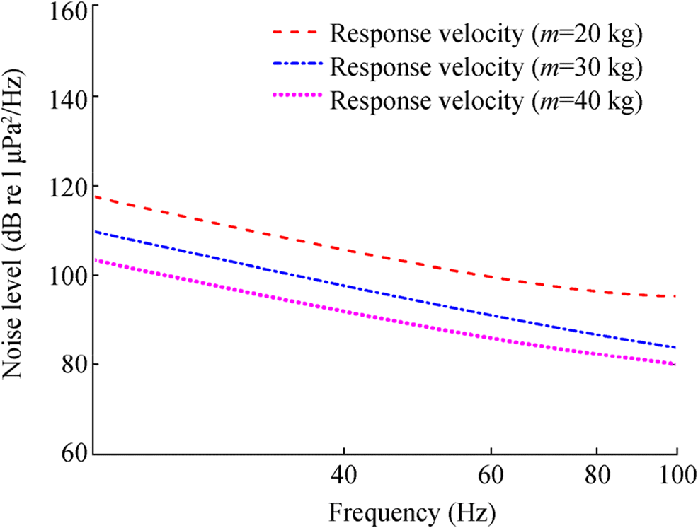Figure  16  The noise level of flow noise under different masses

Download: Full-Size Img

4.3   Different Sea States

Figure 17 shows the response velocities obtained under different sea states when k = 5 N/m and m = 20 kg. The results show that while the elastic constant and mass keep unchanged, the amplitude of response velocity is larger when the sea state becomes worse. This is because the wave period of the sea wave is gets larger as the sea state becomes worse.

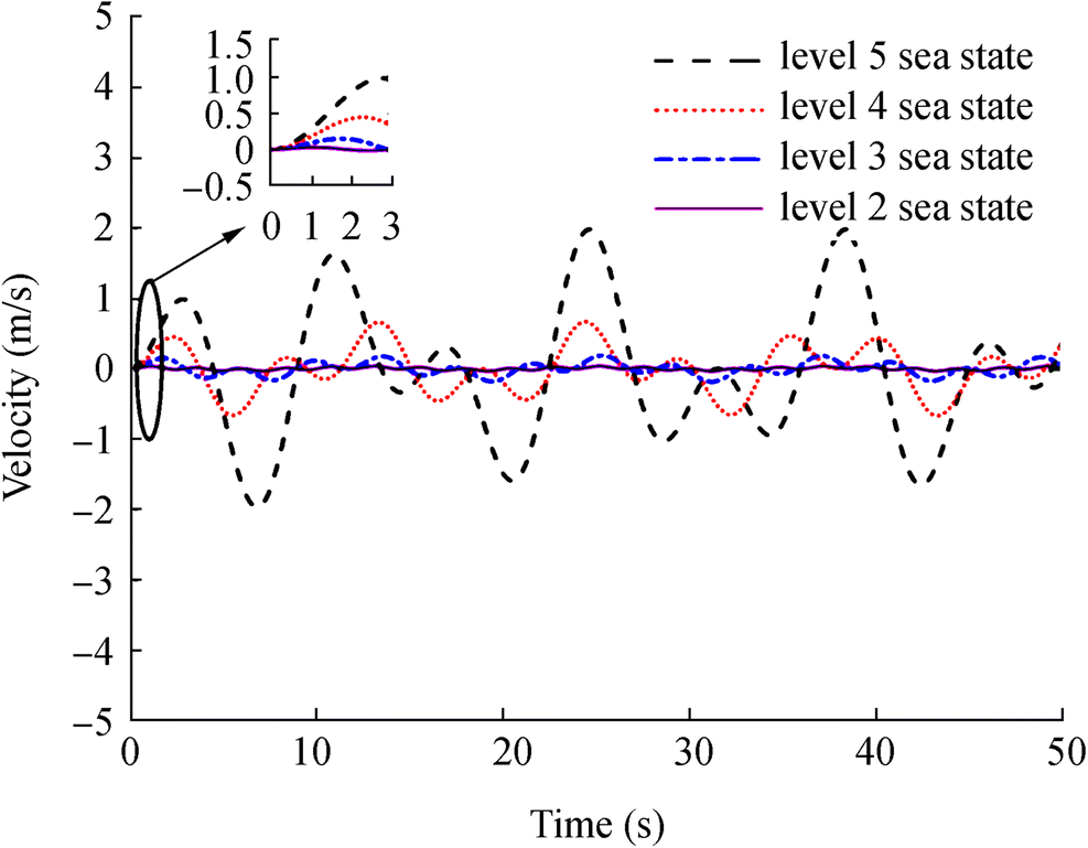Figure  17  Response velocity under different sea states (k = 5 N/m, m = 20 kg)

Download: Full-Size Img

Figures 18(a)-(d) depict the wall pressure fluctuations on the hydrophones, which were calculated by taking the response velocities obtained under different sea states as the inflow boundary conditions. Here, it should be noted that k = 5 N/m and m = 20 kg.

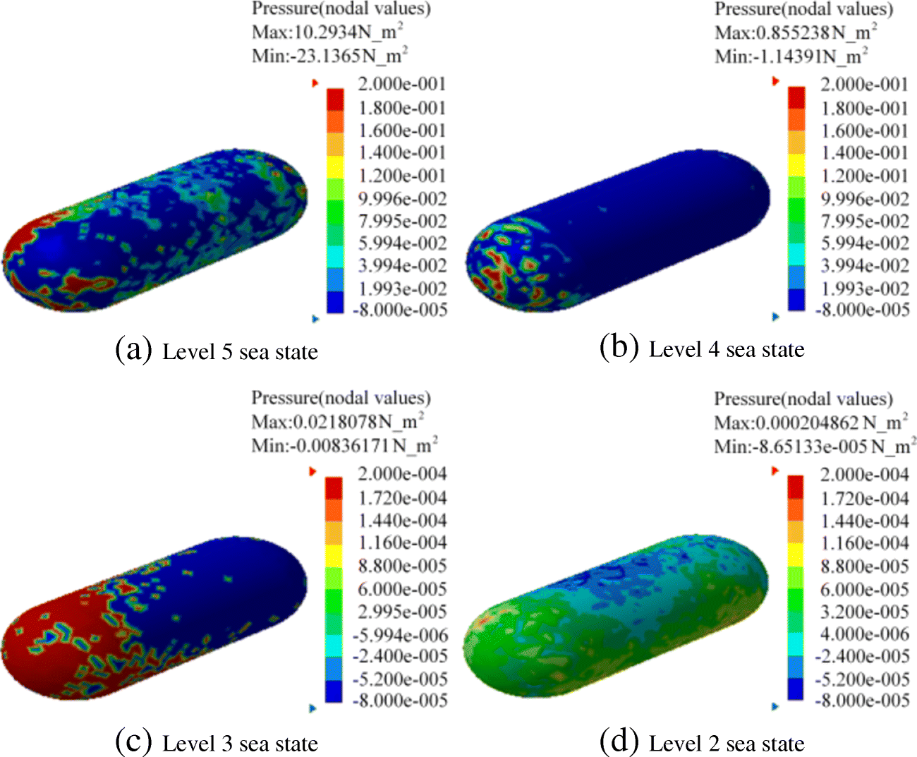Figure  18  The pressure fluctuation on the wall of hydrophone under different sea states (20 Hz)

Download: Full-Size Img

(a) Level 5 sea state (b) Level 4 sea state

(c) Level 3 sea state (d) Level 2 sea state

Figure 18 shows that when the elastic constant and mass keep unchanged, the pressure fluctuations on the wall of the hydrophone will gradually increase as the sea state deteriorates. The pressure fluctuations in Fig. 18 were taken as the noise source in the calculation of the acoustic response with FW-H equation. The result is shown in Figure 19. It is indicated that the noise level of the flow noise becomes larger as the sea state becomes worse.

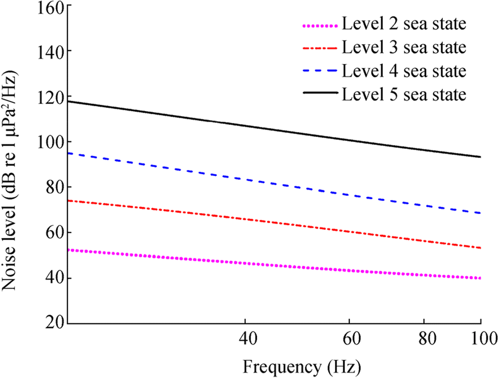Figure  19  The noise level of flow noise under different sea states

Download: Full-Size Img

5   Conclusion and Discussion

In this study, a suspension system which consists of an elastic suspension cable and isolation mass was used to suppress the vertical motion of the sonobuoy. A theoretical model of motion based on the suspension system of the sonobuoy was given. The velocity responses of the optimized sonobuoy under different conditions were obtained by solving the dynamic differential equation. The suppression effects on hydrophone vertical motion of the elastic constant, the mass of the sonobuoy underwater part and the wave period were analyzed, respectively. Combining the theoretical model of motion, a hybrid numerical computation method based on CFD and FW-H was employed to compute the flow noise of the sonobuoy. The predicted flow noise can be used to evaluate the suppression effect of the suspension system on hydrophone vertical motion.

The main conclusions are obtained as follows:

(1) The suppression effect of the suspension system on the vertical motion of the hydrophone is mainly affected by elastic constant, mass, and wave period. Smaller elastic constant and larger mass can suppress the transmission of vertical motion better.

(2) Smaller transmission rate means better suppression effect, and the transfer rate is less than 1 while the ratio of ω_n and ω is smaller than 0.578.

(3) The hybrid numerical computation method for predicting the flow noise has good calculation accuracy. The simulation result was verified by the experiment data and empirical formula.

(4) The simulation results show that the suspension system has a good effect on reducing the flow noise of the sonobuoy caused by its vertical motion. At last, the experiment to confirm the vertical motion suppression effort and verify the flow noise of the sonobuoy computed by the numeral calculations will be the future work.