1   Introduction

Exhaust gas emissions from ships present a key issue in the environmental impact assessment of maritime transports (Boselli et al. 2019). The contribution of maritime traffic to global emissions is estimated to be 938 million tons of carbon dioxide (CO₂), 5.6 Tg of nitrogen oxides (NO_x), and 5.3 Tg of sulfur oxides (SO_x) (MEPC 2014; Murena et al. 2018; Smith et al. 2014). Ships emit pollutants during cruising at sea and maneuvering and mooring phases at ports. While emissions at sea need to be assessed for their impact on a global scale, in particular, as regards greenhouse gases, ship emissions in port areas may propagate to nearby urban areas, affecting the air quality and jeopardizing people's health and quality of life (Adamo et al. 2014; Ault et al. 2009; Quaranta et al. 2012; Viana et al. 2014). Although local emissions are a small fraction of global transport emissions (Entec UK Limited 2002), they can have serious effects on human health, especially in coastal areas and water cities.

Diesel engines used as the main power supply of marine vessels produce a range of emissions, including carbon monoxide (CO), carbon dioxide (CO₂), nitrogen oxides (NO_x), sulfur oxides (SO_x), hydrocarbons (HC), and particulate matter (PM) (Heywood 1988; Eyring et al. 2005; MEPC 2014). The most relevant limits are certainly those related to the percentage of sulfur content (SO_x) in marine fuels and emissions of nitrogen oxides (NO_x) from engines.

The regulation of pollutants from maritime traffic is the subject of the International Convention for the Prevention of Pollution from Ships (MARPOL) 73/78 Annex VI, a legislation issued by the International Maritime Organization (IMO) (Murena et al. 2018). Annex VI (added in 1997 and entered into force in May 2005) regulates air pollution from ships by dealing with SO_x, NO_x, and PM from exhaust gases, shipboard incineration, and emissions from volatile organic compounds. The original Annex VI of the convention has undergone successive changes aimed at reducing the limits related to the emissions of the nongreenhouse gas pollutants based on the technological improvements made over the years and the ever more severe need to decrease emissions (IMO 2007; IMO 2008).

For NO_x, the reference standards are the Tiers I, II, and III, which are calculated according to the revolutions of the engine (r/min) and depending on the ship's date of construction (IMO 2008). Nowadays, the reference is Tier II, whereas Tier III is to be considered valid only in the NO_x emission control areas (IMO 2007).

The study on emissions related to marine traffic can be tackled from different points of view: On the one hand, it is possible to perform monitoring campaigns (Cooper et al., 2001; Prati et al. 2015) of a ship engaged in port operations and then analyze the dispersion of pollutants in the atmosphere. On the other hand, the emission sources can be characterized with simulation models representing the diesel engine in the various stages of a ship's operation, relating them to the weather conditions and loading of the engine (Prpic-Orcic et al. 2016).

In the study by Dobrucali and Ergin (2019), a numerical study on the effects of operational conditions, design parameters, and buoyancy on the exhaust smoke dispersion of a generic frigate are presented and discussed. In the study by Kalender and Ergin (2017), an experimental investigation of the particulate emission characteristics emitted by a medium-speed diesel engine installed on a ferry is reported. The two approaches intersect to validate simulation data with real data.

Simulation has been used in engineering for many years as support of design and manufacturing (Altosole et al. 2012; Tadros et al. 2020a). Marine propulsion system simulations can be used for many purposes, such as ship performance analysis (Campora and Figari 2003; Figari and Soares 2009; Acanfora and Cirillo 2017), maneuvering analysis (Benvenuto et al. 2000; Altosole et al. 2013; Piaggio et al. 2019; Ircani et al. 2016), machinery control system development (Altosole et al. 2007; Michetti et al. 2010), and machinery performance analysis (Maftei et al. 2009; Zaccone et al. 2015; Altosole et al. 2019; Tadros et al. 2020c).

The elements within a classic propulsion simulation model are the hull model, propeller model, engine model, and governor. The "engine model" normally consists of the following main subsystems: cylinder, inlet and outlet manifold and intercooler, compressor, turbine, and shaft dynamics. Diesel engine simulation models can be classified into three categories: zero-dimensional (0D) single-zone models, quasi-dimensional multi-zone models, and multidimensional models (Chidambaram and Thulasi 2016). 0D single-zone models assume that the cylinder charge is uniform in composition and temperature at all times during the cycle (Heywood, 1986). Although this model has the capability of accurately predicting engine performance, it has a limitation in the prediction of exhaust emissions.

Multidimensional models, such as KIVA (Amsden et al. 1985; Amsden et al. 1987), model the volume of the cylinder with a fine grid, providing a formidable amount of special information. However, the results may vary according to the formulation of initial or boundary conditions, which take a lot of computation time. As an intermediate step between 0D and multidimensional models, multi-zone models can be effectively used to model diesel engine combustion systems (Chidambaram and Thulasi 2016).

The quasi-dimensional models combine some of the advantages of 0D and multidimensional models. They solve mass, energy, and species equations but do not explicitly solve the momentum equation. These models can provide the spatial information required to predict emission products and require significantly less computing resources compared to multidimensional models.

Among the multi-zone models, the simplest and most effective one is the two-zone model that splits the cylinder into a nonburning zone of air and another homogeneous zone where fuel is continuously supplied from the injector and burned. According to Ishida et al. (1996), a significant improvement in the prediction of the in-cylinder phenomena is represented by the "two-zone" approach, which provides distinct calculations for the burning and nonburning zones. This combustion model, unlike the 0D model, allows evaluating gaseous emissions with semi-empirical equations and is used for predicting the performance and emission characteristics of a conventional engine. In particular, the "single-zone" combustion scheme is not suitable for the evaluation of exhaust emissions because it does not calculate the flame temperature, whose value is required by the semi-empirical relations providing NO_x and soot formation and oxidation rates (Altosole et al. 2017).

The formation of nitric oxide is controlled by chemical kinetics, and as well known, according to the thermal Zel'dovich mechanism (Zel'dovich 1946), a high combustion temperature is responsible for an increase of the production of nitrogen oxides (Raptotasios et al. 2015; Altosole et al. 2017). Some authors, such as Raptotasios et al. (2015), approach the problem of NO_x production through the adoption of the extended Zel'dovich mechanism (Lavoie et al. 1970; Heywood 1988). According to Trodden and Haroutunian (2018), NO_x production is predominantly a function of engine speed (or residence time) and loading. Zel'dovich (1946) provided a mechanism to estimate the thermal NO formation. This approach has a limited number of reactions: It can be challenging in estimating required oxygen concentration and is relatively fast for computation.

An interesting approach is the chemical kinetics analysis, which can accurately model the production of NO_x and other species and can be embedded into a numerical engine model to provide estimates of emissions under varying loading conditions. The use of chemical kinetic solvers allows the analysis of how different conditions can influence the speed of reactions and yield details about the mechanism and transition states of a reaction. Some chemical kinetic solvers have been formulated, including ChemKin (Reaction Design 2017), Cantera (Goodwin et al. 2009), and the Kinetic PreProcessor (Damian et al. 2017).

Tadros et al. (2015) used an engine model of a two-stroke diesel engine in conjunction with a chemical kinetic routine to estimate exhaust emissions. The results obtained were validated through data from real engines. In the simulation performed by Trodden and Haroutunian (2018), an emission factor was developed using a numerical engine model coupled with chemical kinetic computations. The same model, coupled to a ship's maneuvering simulator, was then used to compare NO_x formation during maneuvering operations. The results demonstrated that, during maneuvers, the developed simulator exhibits significant differences in NO_x formation, compared to the commonly used emission factor approaches.

In the study by Tadros et al. (2015), the element potential method (Kristensen 2012) was used to calculate the chemical equilibrium of the combustion equation to determine the mole fraction equilibrium for the combustion products of all species and then to calculate the NO_x and CO₂ rates. The results show a good fitting between the rates of NO_x calculated from the combustion process and those calculated using the emission factors (Kristensen 2012), as a function of the specific fuel consumption (SFC). Finally, the NO_x emission showed a total dependence on the maximum temperature of the combustion process. In the study by Tadros et al. (2016), the CO₂ and NO_x emissions were calculated from the equilibrium of the equation of combustion for different start angles of combustion. In the studies by Tadros et al. (2018) and Vettor et al. (2018), a fourth-order polynomial regression model implemented in MATLAB was used to generate an equation of CO₂ and NO_x emissions from two four-stroke marine turbocharged diesel engines.

Another interesting research development found in the literature is the adaptive neuro-fuzzy inference system (ANFIS) models, capable of solving nonlinear problems. ANFIS, a hybrid intelligent system coupled with a fuzzy logic system with an artificial neural network, has the advantage of being adaptable and effective for nonlinear complex problems. Hosoz et al. (2013) developed an ANFIS model to predict the performance parameters and exhaust emissions of a diesel engine, and the results showed a good agreement with experimental data. In the study by Tadros et al. (2020d), the ANFIS model was recommended to be further used to investigate the exhaust emissions of engines and to be coupled with other software for optimization procedures.

Moreover, an optimization tool was adopted to monitor and optimize a few engine performance parameters without the need for tests and experimental measurements (Tadros et al. 2016). Tadros et al. (2019) developed a numerical optimization model to simulate the performance of a large four-stroke marine turbocharged diesel engine in the entire operating range and to identify optimal values for adjustable parameters, such as the speed of the turbocharger and start angle of injection. In another study, Tadros et al. (2020b) developed an engine optimization model to fit the calculated in-cylinder pressure diagram to experimental data by finding the best-fitting values for the start angle of injection and the amount of injected fuel for different engine loads. The same methodology can be used for fitting the performance characteristics of numerical models of further engines.

The rest of this paper is structured as follows: In Section 2, the methods, software adopted, and case study, including ship and engine data, are described. In Sections 3 to 4, the results of the engine bench tests and vessel sea trials are presented. In Section 5, the structure of the model is described. In Section 6, the results (calibration, validation, and comparisons with actual data) and discussions are presented. Finally, in Section 7, conclusions and future developments are presented.

2   Methods

2.1   Adopted Software

The simulation software used is RICARDO WAVE, which is a state-of-the-art one-dimensional (1D) gas dynamics simulation tool. It is used worldwide in industrial sectors, including rail, marine, and power generation. WAVE enables performance and acoustic analyses to be performed virtually for any intake, combustion, and exhaust system configuration. The simulation software solves the 1D form of the Navier-Stokes equations governing the transfer of mass, momentum, and energy for compressible gas flows and includes submodels for combustions and emissions. WAVE contains advanced combustion models for diesel engines and includes secondary models specific for the study of engine-out emissions and knocking combustions.

2.2   Case Study

The software has been used for the construction of a simulation model capable of predicting the performance and emissions of a marine diesel engine (MTU39616VTE74L), for which measurement at the test bench and experimental measurement, during the ship navigation, are available. The experimental campaign was performed onboard a catamaran owned by Caremar, the navigation company between Naples and nearby islands.

The catamaran features a propulsion system, including two S71 Kamewa waterjets (SII waterjets, 860 r/min), a displacement of 137 t, and accomodation of up to 354 passengers. The principal characteristics of the ships (http://www.naviecapitani.it) are presented in Table 1.

The total power installed onboard is attributed to the two diesel engines of MTU39616VTE74L.

In the acronyms, "MTU" corresponds to the manufacturer, "16" indicates the number of cylinders, "V" is the shape, "396" is the series number and the displacement of one cylinder (multiplied by 100), "T" is turbocharger with exhaust gas, "E" is the type of air cooling, "7" indicates the use of the engine in maritime application, and "4L" is the serial number.

The turbocharger group consists of a turbine, driven by the exhaust gases of the engine, and a compressor mounted on the same axis. The exhaust gases coming from the cylinders are conveyed to the turbine and, acting on the turbine blades, move the compressor. The compressor impeller sucks in the combustion air, compresses it, and sends it to the cylinders. The main characteristics of the engine are indicated in Table 2.

3   Bench Tests

Bench tests were performed on both engines onboard: the main surveyed engine parameters are the rotational speed (r/min), torque (kNm), power (kW), mass flow rate (kg/h), and SFC (g/kWh). The main results for one of the two diesel engines are shown in Figures 1 and 2.

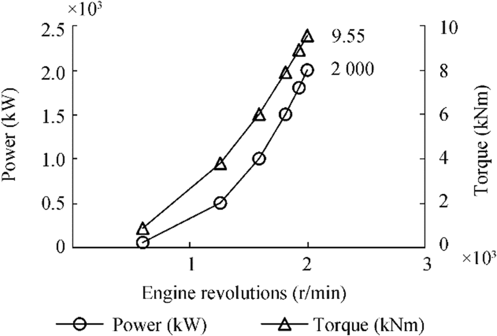Figure  1  Bench test: power and torque

Download: Full-Size Img

Figure  2  Test bench: fuel flow rate and SFC

Download: Full-Size Img

As shown in the graphs, at 2000 r/min, on the measurement bench, a delivered power of 2000 kW was surveyed with an SFC of 221 g/kWh and a torque of 9.55 kNm.

4   Experimental Campaign

The complex data logging campaign has required a very reliable measurement system. The instrumentation was previously tested in the laboratory (for torque and power). In each route, considerable information was logged, with a rate of two samples per second. To supply cross-validation on the logged values of the torque, four flow meters were used to measure the fuel supply and return flow from the pumps. The comparison between the working point in full scale and the one drawn from the bench tests of the engines confirmed the good quality of the data. The ship's position and speed were surveyed by a global positioning system (GPS). The displacement of the ship was evaluated by reading the astern and bow drafts and keeping into account the changes of weight (fuel and passengers). The overall arrangement of the data logging system is given in Figure 3. Each run has been characterized by ship displacement, wind and sea conditions, and ship conditions.

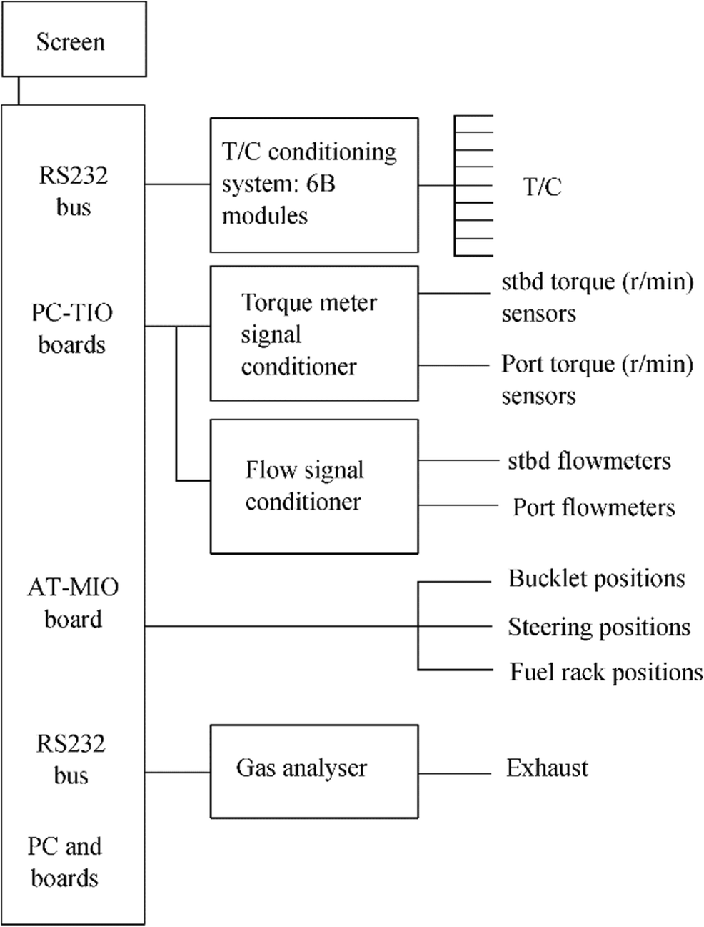Figure  3  Layout of the data logging system

Download: Full-Size Img

The data logging campaigns were conducted on the routes to and from the islands of Procida, Ischia, and Capri. The data logging system was capable of registering the main parameters of the propulsion and navigation. In some cases, an exhaust gas analyzer was used to survey the concentration of the main pollutants in the exhausts. The main characteristics of the data logging system used for the campaigns are reported in Table 3. The monitored parameters were torque on the propeller shaft (kNm), power (kW), rotational speed (r/min), fuel consumption (cm³/s), and exhaust gas temperature (℃). The pollutants measured, i.e., HC (ppm), CO (%vol), CO₂ (%vol), and NO_x (ppm), were measured together with the concentration of O₂ in the air. Because both vessels work with low-sulfured fuels, SO_x was not recorded (Cooper 2001).

In Figure 4, just as an example of the available data, torque and power are recorded during an entire route: the left vertical axis reports power, and the right one torque.

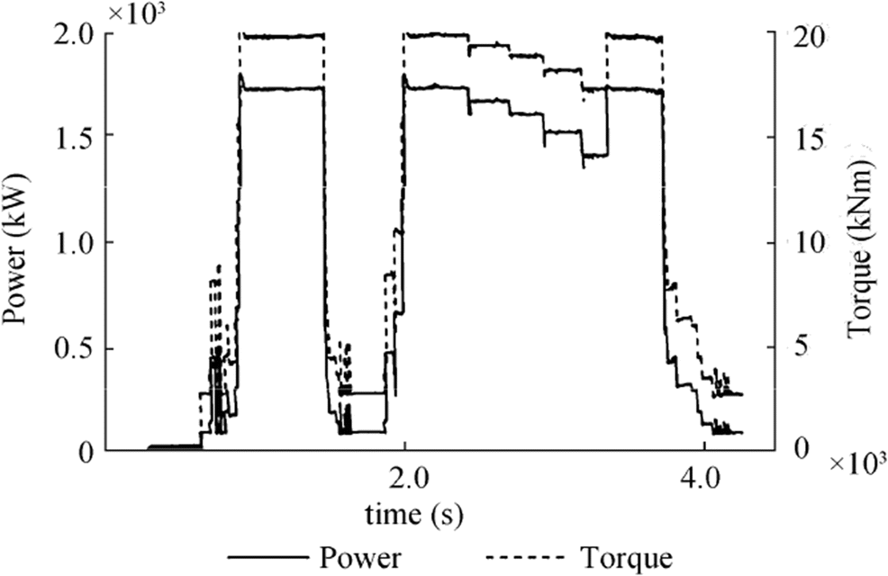Figure  4  Experimental campaign—examples of time histories

Download: Full-Size Img

5   Model Structure

The model built within the Ricardo WAVE environment consists of the following elements: engine, cylinders, valves, injector, charge air cooler, turbocharger (turbine, compressor, and shaft), ducts, and y-junctions.

An overall view of the simulation model is reported in Figure 4. In the top center area, the engine block is connected with all the cylinders, which are distributed on two banks, left and right. Each cylinder features four valves and a direct injector on the top. A mass flow rate injector element delivers a specified amount of fuel per unit time, following a user-defined profile. The turbocharger group is linked to the ambient (clouds on the top center), the compressor is linked respectively to the two intercoolers, and the turbine is connected to the exhaust gas manifold and with the ambient in exit (clouds on the down center) (Figure 5).

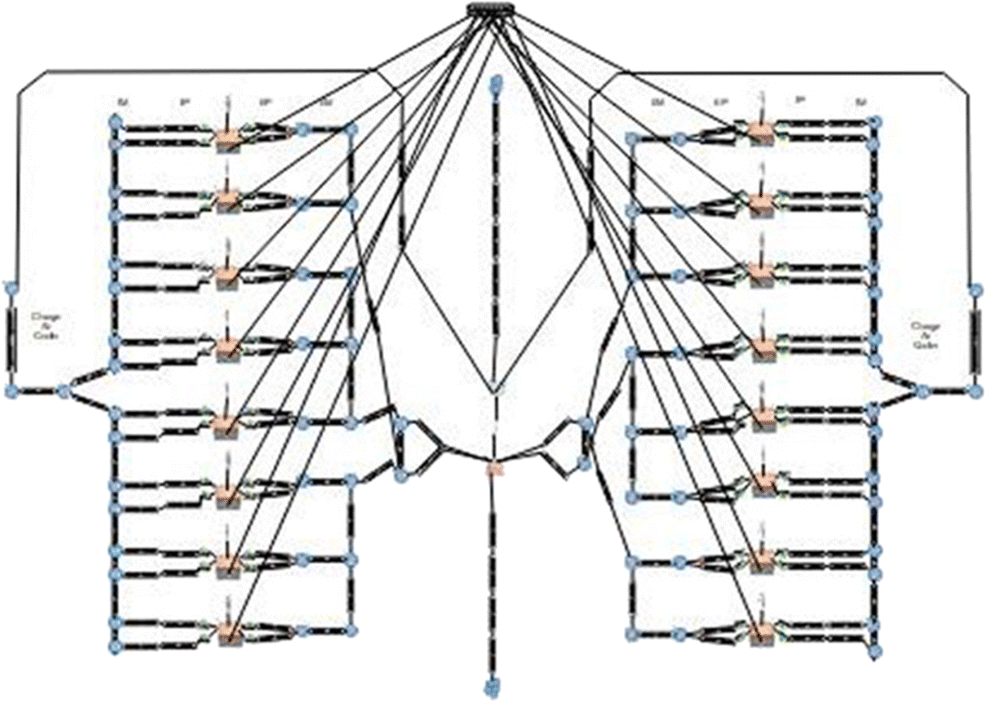Figure  5  Simulation model

Download: Full-Size Img

Each cylinder is connected to the engine with its ignition order, to the valves, and the injector. The cylinders are then connected to the turbocharger and intercooler through ducts characterized by the length and diameter. An example of a single line is shown in Figure 6, where the cylinder, valves, injector and inlet, and outlet ducts can be identified.

Figure  6  Details of a single-cylinder model structure

Download: Full-Size Img

In the absence of details about the turbocharger (except for a maximum speed of 60 000 r/min), as a standard procedure in these cases, turbine and compressor maps were adopted, belonging to an engine with the same number of cylinders and the same V shape but different displacement (50 L instead of 63.3 L). These maps are scaled to fit our engine. The two-zone Wiebe diesel model was used to capture in more detail the processes taking place during the combustion phase.

The Wiebe function was used to estimate the mass fraction burned as a function of piston position and expressed as (Watson et al., 1980)

where x_b is the mass fraction burned; p_f, d_f, and t_f are the mass fractions of the premix, diffusion, and tail burn curves, respectively; cd₃ and ct₃ are the burn duration coefficients for the diffusion and tail burn curves, respectively; and τ is the burn duration in degrees calculated according to the following expression:

where θ is the crank angle, θ_o is the crank angle as the combustion starts, RPM is the engine speed, and BRPM is the reference engine speed. Using the first law of thermodynamics (Heywood 1988), the change in pressure

and in temperature

along the crank angle are calculated by Equations 3 and 4, where K is the heat specific ratio; V, P, and T are the cylinder volume, pressure, and temperature, respectively; dV/dθ is the change in volume; and dQ is the total heat added.

The original Woschni heat transfer submodel considers the charge as having a uniform heat flow coefficient and velocity on all surfaces of the cylinder. It calculates the amount of heat transferred to and from the charge based on these assumptions. It is the most commonly used heat transfer submodel and can be applied to all cylinder elements. The Woschni heat transfer coefficient is calculated using the following equation:

where D is the cylinder bore; P and T are the cylinder pressure and temperature, respectively; v_c the characteristic velocity; and C is the multiplier.

The characteristic velocity is the sum of the mean piston speed and an additional combustion-related velocity, which depends on the difference between the cylinder pressure and the pressure that would exist under motoring conditions.

At each step during the combustion phase, the mole fractions of 11 species were calculated for the unburned and burned zones based on thermodynamic equilibrium and were then averaged. When combustion ends, the single-zone model was used. The NO_x emission submodel predicts the NO_x production during combustion and exhaust in an engine cylinder element. At any instance of the combustion process, a mass flow into the burned zone took place, associated with the instantaneous fuel-burning rate and stoichiometry of the incremental burned mass. The composition of the fresh air introduced into the engine was needed as an input datum, in terms of the molar fractions of oxygen, nitrogen, carbon dioxide, and water. Nitrogen oxide formation was calculated for each fuel/air package separately taking the local temperature. The formation of NO_X emissions was calculated using the extended Zeldovich mechanism, taking into account the two zones of combustion (burned and unburned zones). The Arrhenius multipliers of the following chemical reactions in the NO_x emission model were calibrated depending on the data of NO_x emissions provided from the datasheet of the manufacturer.

The NO_x model accounts for the "prompt" or "flame formed" NO, which is due to the over-equilibrium radical concentration in the flame zone. This quantity was obtained from a correlation, which gives the ratio of prompt NO to equilibrium NO as a function of the equivalence ratio (between the two zones). The overall burned zone is treated as an open and stratified system, in which further NO_x formation takes place in function of pressure, temperature, and equivalence ratio of the burned packet. All the NO_x was assumed to be in the form of NO during the prompt formation phase and thermal phase described by the Zeldovich mechanism of the NO_x formation.

where O, N, and H are the oxygen, nitrogen, and hydrogen atoms and thermodynamic equilibrium values are used for the species O₂, O, H, and OH. The steady-state assumption is used for highly reactive N atoms. The concentration of NO versus time was computed using an open system in which the above elementary reactions were used with the rate constants reported by Heywood (2018). These rate constants are a function of the activation temperature for the reaction, burned zone temperature, and pre-exponential and exponential constants. The calculation was terminated when the temperature in the burned zone reaches a low enough level so that the kinetics become inactive and the total NO no longer increases.

6   Results and Discussion

6.1   Setup and Input to Simulations

Once the model is defined, the second validation step involves simulations at different r/min of the engine, aimed at verifying the congruence of the simulated data with respect to those measured in the experimental campaigns. The basic engine model is a time-dependent simulation of in-cylinder processes, based upon the solution of equations for mass and energy. The mass equation accounts for the changes of the in-cylinder mass due to the airflow through valves and to fuel injection. The energy equation is based on the first law of thermodynamics and equates the change of internal energy of in-cylinder gases to the sum of enthalpy fluxes in and out of the chamber, heat transfer, and piston work.

The simulations were performed while keeping all the blocks of the model active and, as previously mentioned, using the turbine and compressor maps scaled from a similar engine. Simulations were generally 30 s long, except those for low revolution speeds, which were extended to 100 s to absorb any transient of the model. The ambient pressure was set at 1×10⁵ Pa, whereas the ambient temperature was set at 305 K according to an average value measured in the engine room during the measurements.

The duration of the injection was set to 22°, the SOI angle was set to 11° BTDC-, and the SOC was set to 8° BTDC. The fuel/air ratio was set to 0.030. According to the manufacturer's instructions, the injector nozzle diameter was set to 1.1 mm and the spray angle to 152°, which were used to assess the impact area on the wall. The diameters of the inlet and outlet valves were taken from engine drawings and were found to be equal to 75 and 70 mm, respectively. For the lift of the valves, however, the real diagrams were not available. Consequently, the 50-L engine's valves (whose maps were scaled) were spread on the timing angles of the MTU engine (see Table 2).

In this model, two-zone Wiebe diesel and original Woschni heat transfer were chosen. For the NO_x emissions, the Arrhenius pre-exponent multiplier was 1.5, and the Arrhenius relationship rate constant multiplier was 1.0.

A modified form of the Chen-Flynn correlation (engine friction) was used to model the friction in the WAVE engine. For the scavenging, in this model, a "fully mixed" configuration, where the mass leaving the cylinder is a perfect mixture of the mass in the cylinder, was chosen.

The model returns the desired engine parameters, including torque, power, consumption, pollutant flow rates, pressures, and temperatures, for each of the selected case studies. These are the minimum conditions required to get the basic model running. In addition, it is necessary to have temperatures in several locations in the exhaust system as they greatly vary and have a significant effect on the prediction performance.

For these reasons, the model requires a first hypothesis on the temperatures of the average surface temperature of the piston top or crown (T piston) and the average surface temperature of the cylinder liner (T cylinder) and head (T head), which were set at 500 K, 540 K, and 550 K, respectively.

6.2   Calibration

Figures 7, 8, and 9 show the comparisons between the model simulation results and test bench data for SFC, power, and torque, respectively.

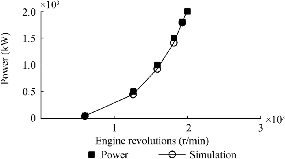Figure  7  Calibration of the model: power

Download: Full-Size Img

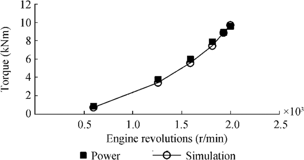Figure  8  Calibration of the model: torque

Download: Full-Size Img

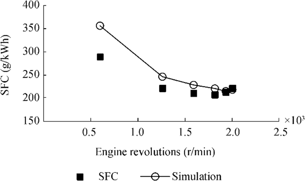Figure  9  Calibration of the model: SFC (g/kWh)

Download: Full-Size Img

Table 4 summarizes the same data in terms of error percentages. All the differences are less than 10% in the medium-high range of engine speeds, so they can be considered as reasonably good.

The discrepancies increased at the engine's low loads, but as an average value, the differences were 7% for the power or torque and 8% for the consumption. Moreover, the error in the power delivered affected the specific consumption because the fuel flow rate is certainly correct as it corresponds to an input to the model.

6.3   Validation

Time-averaged values obtained during sea trials were used as input for the stationary simulation model. Starting from the consumption in g/kWh and from the relative power, the hourly flow rate for each cylinder was obtained.

The flow rate and r/min correspond to the simulation inputs. The extracted average values are presented in Table 5. The specific emissions of NO_x were obtained, according to Heywood (2018), as a function of all the species concentrations, which composed the exhaust gas. The errors for each case are reported in Table 6. As evident from the figure, the power, torque, and SFC from the maximum load of the engine down to approximately 65% have relatively small errors. At low revolutions, the simulation errors increase due to transient events that the measuring instruments and simulation were unable to model properly.

As mentioned above, the error increased with decreasing engine load, as expected. In particular, the average errors related to the torque, power, SFOC, and ppm of NO_x are 11.1%, 11.4%, −20%, and 29.2%, respectively. However, if these average errors are evaluated down to 1400 r/min (approximately 32% of the engine load), these average errors can be reduced to 6.8%, 6.9%, −7.1%, and 8.7%, respectively. These errors, together with the encouraging trend of the points shown in the graphs, make it acceptable to consider the behavior and response of the model in the validation. The simulation results were compared to those of the steady-state conditions. In particular, the power, consumptions, and emissions of NO_x are compared in Figures 10, 11, 12, and 13.

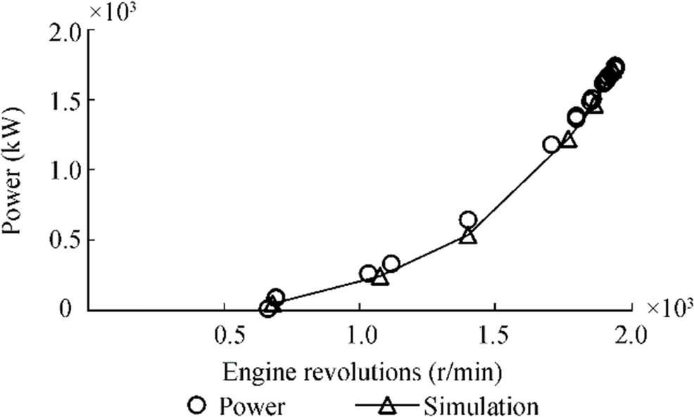Figure  10  Validation of the model—power

Download: Full-Size Img

Figure  11  Validation of the model—SFC

Download: Full-Size Img

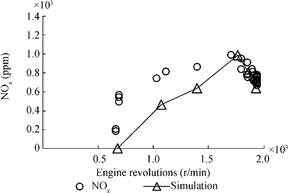Figure  12  Validation of the model: NO_x in ppm

Download: Full-Size Img

Figure  13  Validation of the model: specific emission of NO_x in g/kWh

Download: Full-Size Img

6.4   Discussion

The results obtained in terms of power, torque, and consumption are all good when compared with the experimental tests and the bench tests. As for the emissions, Figures 12 and 13 show that when the revolutions are reduced, the simulation provides results lower than those measured. This fact, for the ppm, is to be linked to errors made in the choice of the typical temperatures in the cylinders. Conversely, the causes for the discrepancies in the emissions in g/kWh can be various: errors in the power estimation performed by the engine simulation model, errors in the methodology and assumptions made for calculating the emission starting from NO_x (ppm) measured at sea, and measurement errors of the instrumentation on board not only as regards the ppm of NO_x but also the other pollutants, which, according to these emissions in g/kWh, were estimated starting from the whole composition of the exhaust gas. Considering a revolution of 2000 r/min and the ship's construction year (before 2000), the regulatory limit for the case study is 9.8 g/kWh. If the rare cases of outlier are excluded, then this emission factor complies with the measurements and simulations obtained (see Figure 12).

7   Conclusions

The development of simulation models for combustion engines with the capability of predicting emissions is an important target in the maritime sector, considering the commitment to reduce emissions on local and global scales. This article presents a simulation model of a four-stroke diesel engine used in the maritime field. The simulation results were calibrated with engine bench tests and validated with experimental tests at sea. The results obtained under stationary conditions showed a good fit with data from an experimental campaign performed on board, which encouraged us to test the model in other situations, characterized by transient situations during maneuvers. Further applications will study in-depth the transient operating phases of the engine operation, the interface between the simulation models, the automatic identification system data of vessels on a specific route, and a predictive emission estimation method based on emission factors as a function of the type of engine, fuel, and pollutants. Future developments of the model will include an interface with the SIMULINK environment to integrate the behavior of ships in navigation and ports. Finally, further investigations will adopt the simulation software in search of an equilibrium configuration of a larger number of species in the combustion chamber to evaluate differences in the resolution and quality of the results obtained. The availability of a reliable numerical prediction can allow assessing and controlling emissions in these situations, which represent the largest risk on the health of inhabitants of areas surrounding ports.