Ice Resistance Assessment for a Large Size Vessel Running in a Narrow Ice Channel Behind an Icebreaker
https://doi.org/10.1007/s11804-021-00226-x
-
Abstract
Large size vessels sailing in continuous level ice and broken ice of high concentration are mostly assisted by icebreakers. This is done in order to provide for fast transportation through the North Sea Route and safe operation in extreme ice conditions. Currently, new large size gas and oil carriers and container ships are being designed and built with beams much greater than the beams of existing icebreakers. At the same time, no mathematical description exists for the breaking mechanism of ice channel edges, when such vessels move under icebreaker escort. This paper suggests a simple method for assessment of the ice resistance in the case of a large ship running in an icebreaker channel; the method is based on modification of well-known semi-empirical methods for calculation of the ice resistance to ships in level and broken ice. The main feature of the proposed calculation scheme consists in that different methods are applied to estimate the ice resistance in broken ice and due to breaking of level ice edges. The combination of these methods gives a deliverable ice resistance of a large size vessel moving under icebreaker assistance in a newly made ice channel. In general, proposed method allows to define the speed of a carrier moving in an ice channel behind a modern linear icebreaker and could be applied at the ship design stage and during development of the marine transportation system. The paper also discusses the ways for further refinement of the assessment procedure suggested.Article HighlightsA new method was proposed for ice resistance assessment in the case of large size carriers running in a wide or a narrow ice channel behind an icebreaker.The total ice resistance of vessel running in the ice channel is different for symmetric and asymmetric movement and the greatest difference taking place in the case of small relative channel widths.The developed method of ice resistance definition and possible versions of large size vessel movement in an ice channel are verified by model test data obtained in the ice basin of the Krylov State Research Center. -
1 Introduction
Large ice-going carriers are one of the key elements in marine transportation systems for Northern Sea Route. The new icebreaking carriers are being tailored to the transportation needs of new Arctic projects, with special emphasis on year-round operation in the eastern sector of the Northern Sea Route. A fleet of such carriers will be used to transport the products from the oil and gas fields primarily to the worldwide markets.
Ice operation of these ships can be autonomous or icebreaker-assisted. In the first case, large carriers move either conventionally, i.e. bow forward, or vice versa, stern forward. The astern moving technique is mostly used by so-called double-acting ships (Backstrom et al. 1995; Wilkman et al. 2004). However, autonomous navigation in thick ice often takes a lot of time, even for double-acting ships. Meanwhile, fast ice navigation of carrier ships is an urgent market demand. Otherwise, the delivery of products through the Suez Canal is more economically viable. Therefore, ice operation studies of large carriers at high speeds, more than 8.0 kn, have now become a whole new research field (Dobrodeev and Sazonov 2018).
One of the possible ways to accelerate ice navigation of carrier ships is icebreaker assistance. It could be implemented in two ways: traditional assistance by one icebreaker, when the ice channel is equal to the hull beam of the icebreaker by two icebreakers (Sazonov and Dobrodeev 2014), when a wide ice channel filled with ice floes is created.
However, two icebreakers mean higher freight costs. So, it would be relevant to consider the one-icebreaker option, which makes a detailed study of this tactic scenario extremely important. As compared to the assistance of ships with small beams, icebreaker assistance of large size vessels has a number of specific features. Some of them arise from the high speed of navigation in ice conditions. An attempt to accelerate ice navigation of large size vessels would require modifications in the design requirements of their hull lines.
The purpose of this study is the development of an ice resistance calculation method for a large size ship moving in a channel behind an icebreaker. A special feature of this method consists in that it renders possible assessment of the ship ice resistance in a channel whose width is less than the ship beam. The study was performed within the framework of the project "Technology for tactical and operational control of icebreakers and ice-class vessels under the conditions of year-round navigation along the Northern Sea Route". The main goal of this project is to develop the scientific and methodological basis for addressing the tactical and operational planning tasks of ship and icebreaker navigation in the Arctic. The obtained solutions should be helpful for assessing the efficiency of various tactical scenarios to support year-round operation of the fleet, which is required for long-term planning of Arctic transportation.
The method developed here is based on a modification of existing semi-empirical techniques for the calculation of ship ice resistance in level and brash ice. The method is verified by model test data obtained in the ice basin of the Krylov State Research Center.
2 Some Features of an Operation Involving Large Size Vessels in the Ice Channel Made by an Icebreaker
There are two possible versions of large size vessel movement in the ice channel made by an icebreaker:
If the channel width is comparable to the carrier beam, it will be running in broken ice. This is a traditional scheme of icebreaking assistance. Dobrodeev (2018a) suggests an ice resistance calculation procedure for this scenario, updated as per the series of tests performed in the Ice Model Tank of the Krylov State Research Center—KSRC (Timofeev et al. 2015).
If the channel width is too narrow, the stem of the carrier will interact with broken ice, and both bow shoulders will break the ice channel edges. This interaction pattern will take place if the ship moves in the channel "symmetrically", i.e. along its central axis.
However, Dobrodeev et al. (2018b) describes a new situation, when a large size vessel moves in a narrow channel "asymmetrically". This means that only one bow shoulder (on the port or the starboard side) breaks the ice channel edge. This scenario characterizes the movement in an ice channel of large size carriers with straight sides of parallel midbody.
The effect of the vessel's asymmetric position in an ice channel behind an icebreaker was discovered during self-propulsion model tests in an ice model tank and later confirmed by the reports of nuclear icebreaker shipmasters. The photo in Figure 1 shows a large size carrier running asymmetrically in an ice channel. Its hull breaks the channel edge at the port side and slides along the other edge along the starboard side. The photo was taken in the spring of 2016 from aboard a nuclear icebreaker leading a 43-m-wide vessel. The ice thickness was 80 cm, and the ice channel width was 28 m. It is difficult to estimate the size and concentration of ice cakes in the wake of the icebreaker in this photo, because from the icebreaker stern, one can see an ice-free water area caused by propeller flushing.
 Figure 1 A large carrier moving asymmetrically in a narrow ice channel
It should be mentioned that this movement scenario is only feasible if the condition of $ B_{C} \ge 0.5B_{S} $, where $ B_{S} $ is beam of the carrier and $ B_{C} $ is the ice channel width, is met. If this condition is not met, the carrier's sides will both interact with level ice edges. This could substantially increase the ice resistance of the carrier, because the icebreaking process will only be due to bow shoulders.
To estimate the navigation speed of large size vessels moving under the assistance of a single icebreaker, it is necessary to develop ice resistance assessment methods for all the aforementioned scenarios.
In view of the above, two calculation scenarios could be formulated for large carrier operations in ice channel (Figure 2).
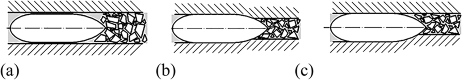 Figure 2 Movement scenarios of large carrier in ice channel: a $ B_{C} \ge B_{S} $; b $ B_{C} \lt B_{S} $, symmetric movement; c $ B_{C} \lt B_{S} $, asymmetric movement
(1) The first scenario takes place when $ B_{C} \ge B_{S} $. Here, the ship practically does not break channel edges (Figure 2a). The bow only interacts with ice cakes in the channel. According to the experience gained from sea trials as well as model tests, it is known that in ice of thickness equal or superior to 1.0 m, the new channel in the wake of the icebreaker is mainly infested with ice cake. The concentration of ice cakes is between 8/10 and 10/10 in the new ice channel. A characteristic feature of this scenario is the ratio between the channel width and the vessel's beam, which results in considerably higher ice resistance because channel edges make it more difficult for the carrier to push ice pieces sideways and sink them.
(2) The second scenario takes place if $ B_{C} \lt B_{S} $. Here, the ship may move both symmetrically and asymmetrically (Figure 2b, c). However, in this scenario, the bow shoulders of the vessel will be breaking one or both channel edges, and some part of the hull will definitely interact with ice cakes.
3 Approach to Ice Resistance Calculation in the Ice Channel Behind an Icebreaker
Today, when coming to the design point, the channel resistance for different ice classes should be considered. The icebreaker-assisted navigation of carriers in ice channels is usually calculated as per the equation developed by Juva and Riska (2002). The resistance equation is expressed in the following form:
$$ R_{{{\text{ch}}}} = C_{1} + C_{2} + C_{3} \left[ {H_{{\text{F}}} + H_{{\text{M}}} } \right]^{2} \left[ {B + C_{\psi } H_{{\text{F}}} } \right]C_{\mu } +\\ C_{4} L_{{{\text{par}}}} H_{{\text{F}}}^{2} + C_{5} \left[ {\frac{{{\text{LT}}}}{{B^{2} }}} \right]^{3} \frac{{A_{{{\text{WF}}}} }}{L} $$ (1) where L is length, m; B is beam, m; T is draught, m; Lpar is length of parallel midbody at waterline, m; AWF is waterline area of the foreship, m2; HF and HM are the ice thickness of the related brash ice layers, m; $ C_{1} $ and $ C_{2} $ are the constants which apply only for ice class IA Super; $ C_{3} = 845.576 $ kg/(m2s2); $ C_{4} = 41.74 $ kg/(m2s2); $ C_{5} $ is implemented according to the data table for different ice classes and brash ice thickness; and $ C_{\psi } $ and $ C_{\psi } $ are the coefficients describing the hull lines.
However, this equation could be obtained only for old ice channels that form in relatively stationary ice after numerous ship passages. As a rule, these channels mostly contain brash ice made up by ice pieces of characteristic size below 2.0 m. In addition, this equation would not include the ice edge breaking process.
In a newly made channel, broken ice pieces have their characteristic size between 2.0 and 20.0 m, depending on the ice thickness. Therefore, an alternative method could be proposed. This method should contain the equations for two components of ice resistance in narrow channel:
– The broken ice resistance component
– The level ice edges breaking component
The approaches for refinement of ice resistance calculation methods for large size vessels were considered by Myland and Ehlers (Myland and Ehlers 2019a, b). Based on assessment of the existing ice resistance prediction method and model tests data, the numerical optimization algorithm was developed. By means of this computer algorithm, the several variables, which were applied to refined version of semi-empirical method, are optimized within specific boundary limits with regard to a minimization of the deviation to the total ice resistance determined by model tests. Such approach made it possible to increase the accuracy of ice resistance prediction. However, in the mentioned research, the approach was developed in relation to the calculation of ice resistance in level ice. In this paper, the movement of large size ship in channel is considered.
3.1 Method for Ice Resistance Calculation When Bc > BS and Bc = BS
As mentioned above, Reference Dobrodeev (2018a) gives an analysis of currently used resistance calculation equations for ships moving in newly made ice channel and derives an analytical expression that updates earlier calculation method suggested by V. Zuev (Zuev 1986). This updated analytical expression is as follows:
$$ {{R}_{BI}}=\frac{\frac{0.63{{\rho }_{I}}g{{B}_{S}}h_{I}^{2}}{{{\left( {{B}_{c}}/{{B}_{s}} \right)}^{{}^{3}\!\!\diagup\!\!{}_{4}\;}}}\left( 0.13\frac{{{B}_{s}}}{{{h}_{I}}}+1.3F{{r}_{h}}+0.5Fr_{h}^{2} \right){{s}^{2}}(2-s)}{1-(0.17-0.58\beta +0.66{{\beta }^{2}})}$$ (2) where s is the ice concentration in the channel, s ∈ (from 0 to 1) (e.g. 0.1 corresponds to an ice concentration 1/10); hI is the broken ice thickness, m; $ \rho_{I} $ is the ice density, kg/m3; $ Fr_{h} = \frac{V}{{\sqrt {gh} }} $ is the Froude number for given ice thickness; $ \beta = \arctan \left[ {\frac{\tan \phi }{{\sin \alpha_{0} }}} \right] $ is the flare angle of the carrier, rad; and $ \alpha_{0} $ is the waterline entrance angle, rad. For bulbous bows, stem angle $ \phi $ must consider the bulbous bow angle at waterline level.
Dobrodeev (2018a) presented a database of ice-basin model tests involving 5 carrier ships with widely different principal dimensions, stem angles, and waterline entrance angles. The main particulars of the ships are presented in the Table 1.
Table 1 Main particulars of considered vesselsCharacteristics Ship 1 Ship 2 Ship 3 Ship 4 Ship 5 Length (m) 299 120 259 75 113 Beam (m) 50 22 35 15.4 24 Stem angle (°) 30 20 20 bulb 60 Waterline entrance (°) 35 40 35 55 45 Ice friction coefficient 0.1 0.1 0.1 0.1 0.1 The tests were performed using FG (fine grain) model ice. To determine the ice resistance of the model hull, KSRC Ice Basin uses the procedure where the model is towed with operating propellers (ITTC No. 7.5 – 02-04-02.2, 2017). The processing of test results and their extrapolation to full scale was performed as per the procedure developed by the KSRC Ice Basin. An ice channel is formed after level ice tests. A part of the ice sheet was broken into ice floes of desired size which moved toward this channel. A layer of small ice pieces forms a broken ice channel. Ice tests are performed at different ship speeds. One of the ships has a bulbous bow.
Calculation results obtained as per modified Eq. (2) have been compared versus the data of the aforementioned model tests. The results of comparison are illustrated in Figure 3 in the form of the relative deviation of experimental data and calculation results obtained as per Eq. (2). Each case refers to a certain channel width and ship speed modelled in the ice tests. Details of the studied scenarios are described by Dobrodeev (2018a).
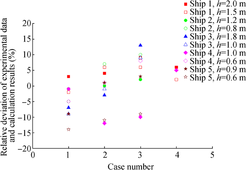 Figure 3 Relative deviation of experimental data and calculation results obtained as per Eq. (2)
The obtained results confirm that Eq. (2) represents quite a satisfactory description of the ice resistance to a carrier running in a new channel with broken ice.
3.2 Method for Calculation of the Broken Ice Resistance Component When Bc < BS
To calculate ice resistance in broken ice for the second scenario when the channel width is smaller than the carrier beam, Eq. (2) has to be slightly modified. It is necessary to assume $ {{B_{C} }/{B_{S} }} = 1 $.
This assumption is made because the hull beam is always wider than the ice channel beam in the analysed scenario of carrier piloting. The total ice resistance is the sum of the broken ice resistance component and of the component of level ice edge breaking. The ice resistance component due to interaction with broken ice is estimated by the modified V.A. Zuev equation and only for the hull part that interacts with broken ice.
To calculate the ice resistance in broken ice, when the ship beam is larger than the channel width, a notion of the "effective hull beam" is introduced. The effective beam Be is the hull part which interacts with broken ice in the channel but does not break ice edges.
For the symmetric case, the effective hull beam is assumed to be $ B_{e} = B_{C} $. Then, to define the component of ice resistance in broken ice, RBIsymm, the calculation Eq. (2) can be written as follows:
$$ R_{{{\text{BIsymm}}}} = \frac{{0.484\rho_{I} gB h_{I}^{2} }}{{1 - (0.17 - 0.58\beta + 0.66\beta^{2} )}},\\ \left( {0.13\frac{B }{{h_{I} }} + 1.3{{Fr}}_{h} + 0.5{{Fr}}_{h}^{2} } \right) \cdot s^{2} \cdot (2 - s) $$ (3) To calculate the ice resistance when a vessel moves asymmetrically, the hull resistance is assumed to be the sum of two components:
– Half-resistance of the hull where the beam is BC
Resistance of the hull where the beam is ${B_{C} - \frac{{B_{S} }}{2}}$
As result, for the asymmetric case, the effective hull beam should be represented as a sum of the mentioned components $ B_{e} = \frac{{B_{C} }}{2} + \left( {B_{C} - \frac{{B_{S} }}{2}} \right) $.
Then, the broken ice resistance for the asymmetric case can be calculated as:
$$ R_{BI \text asymm} = \frac{{0.242 \cdot \rho_{I} gh_{I}^{2} }}{{1 - (0.17 - 0.58\beta + 0.66\beta^{2} )}} \cdot s^{2} (2 - s) \\ \cdot \left[ \begin{gathered} B_{s} \cdot \left( {0.13\frac{{B_{s} }}{{h_{I} }} + 1.3{{Fr}}_{h} + 0.5Fr_{h}^{2} } \right) + \hfill \\ + \left( {2B_{c} - B_{s} } \right) \cdot \left( {0.13\frac{{2B_{c} - B_{s} }}{{h_{I} }} + 1.3{{Fr}}_{h} + 0.5{{Fr}}_{h}^{2} } \right) \hfill \\ \end{gathered} \right] $$ (4) 3.3 Method for Calculation of the Component of Ice Edge Breaking Component of Ice Resistance When Bc < BS
Ice resistance due to the breaking of channel edges can be conveniently calculated as per semi-empirical methods developed for ice resistance calculations in level ice. The six semi-empirical level ice resistance prediction methods are considered in detail in Ref. Erceg and Ehlers (2017). The calculations are made for ships of different sizes and bow shapes. It is found that their deviation from the measurements varies substantially with the ship size. The methods show significant discrepancies. Thus, the method for calculation of the component related to the breaking of channel edges needs to be validated. However, the purpose of this work is mainly to study the specifics of hull/ice interactions in a narrow channel. The fracture mechanics of channel edges is a topic of separate investigations. Therefore, the method developed by B. Ionov (Ionov 1988) is proposed for calculation of the ice resistance. It gives an analytical representation of the hull shape, which makes it possible to provide a detailed description of the hull part interacting with ice in the case of asymmetrical and symmetrical positions of a ship in a channel by calculations within the developed scheme. According to this method, the ice resistance is calculated as follows:
$$ \begin{aligned} R_{I} & = 0.011\sigma_{f} h_{I}^{2} \left[ {a_{1} \left( \beta \right)B_{S} + 2f_{d} a_{2} \left( \beta \right)L^{\prime}} \right] \\ & + 0.15\left( {\rho_{w} - \rho_{I} } \right)gh_{I} B_{S} L^{\prime}\left( {\frac{{\tan \alpha_{0} }}{{\tan \alpha_{0} + \frac{{B_{S} }}{{2L^{\prime}}}}}} \right) \cdot \\ & \cdot \left[ {\alpha_{1} \left( \beta \right)\sin \alpha_{0} + f_{d} \alpha_{2} \left( \beta \right)\left( {1 + \cos \alpha_{0} } \right)} \right] \\ & + 0.7\rho_{I} gh_{I} B_{S}^{2} Fr_{B} \left( {1 + \frac{1}{{\cos \alpha_{0} }}} \right)\left[ {\frac{{\tan^{2} \alpha_{0} }}{{2\tan \alpha_{0} - \frac{{B_{S} }}{{2L^{\prime}}}}} + f_{d} } \right] \\ & + \left( {\frac{{B_{S} - 2T}}{{B_{S} + 2T}}} \right)\left( {\rho_{w} - \rho_{I} } \right)gh_{I} B_{S} \,L_{{{\text{PM}}}} \\ \end{aligned} $$ (5) Here, $ \sigma_{f} $ is the limit bending strength of ice; $ L^{\prime} $ is the length of ship bow; T is the draught; LPM is the length of parallel midbody; $ f_{d} $ is the dynamic coefficient of ice friction against hull plating; $ \rho_{w} ,\rho_{I} $ is the densities of water and ice; $ Fr_{B} = \frac{V}{{\sqrt {gB_{S} } }} $ is the Froude number for given hull beam; $ \alpha_{0} $ is the entrance angle; and $ \alpha_{1} \left( \beta \right),\alpha_{2} \left( \beta \right) $ are special functions characterizing the hull shape and depending on the frame angles along the entrance and determined by the following expressions:
$$ a_{1} \left( \beta \right) = \frac{1}{n}\sum\limits_{i = 0}^{n} {\frac{0.57}{{\sin \beta_{i} }}\left( {1.6\cos \beta_{i} + 0.11} \right)} ;\,a_{2} \left( \beta \right) = \frac{1}{n}\sum\limits_{i = 0}^{n} {\frac{1}{{\sin \beta_{i} }}} , $$ (6) where n is the number of frames within the entrance, needed to calculate shape functions, and i is the number of current frame. For ships with short entrances, functions $ \alpha_{1} \left( \beta \right),\alpha_{2} \left( \beta \right) $ can be obtained with greater accuracy by specifying frame angles with an interval equal to ½ or ¼ of station spacing.
To apply the Ionov method for calculation of the ice edge breaking component of the ice resistance when the carrier moves symmetrically in an ice channel:
– Make a new hull lines, with the beam BS reduced by the channel width BC.
– Determine a waterline entrance angle α0 at the point of its contact with the channel edge.
– The functions dependent on frame station angles α1(β), α2(β) are calculated for the interval from the hull contact point with the channel edge to the point of the maximum beam.
– Update a bow length L′ accordingly.
To apply the Ionov method for calculation of the ice edge breaking component of the ice resistance when the carrier moves asymmetrically in the ice channel:
– The resistance is obtained only for the side that breaks the channel edge.
– Calculation results have to be divided by 2.
The Ionov method only yields ice resistance. But in the case of asymmetric movement, there exist a lateral force and a friction force on the ship side which is located in the ice channel (the starboard side in Figure 5). This side interacts with the channel edge, but does not break it by bending. The lateral force could be calculated using one of Shimansky coefficients $ \eta_{2} $, determined by the following expressions (Kashtelyan et al. 1972):
$$ \eta_{2} = \frac{{\sum\nolimits_{I} {} }}{{\sum\nolimits_{III} {} }};\sum\nolimits_{1} { = k\int\limits_{0}^{{L^{\prime}/2}} {\frac{{\cos x^{\prime}\cos y^{\prime}}}{{\cos \alpha^{\prime}}}} {\text{d}}x;} \,\sum\nolimits_{III} { = k\int\limits_{0}^{{L^{\prime}/2}} {\frac{{\cos^{2} x^{\prime}}}{{\cos \alpha^{\prime}}}} {\text{d}}x;} $$ (7) where $ \sum\nolimits_{I} {} ,\sum\nolimits_{III} {} $ represent the total transverse and longitudinal forces, respectively, on one side; $ {\text{Cos}} x^{\prime},{\text{Cos}} y^{\prime} $ are the respective cosines of angles between the normal to the waterline at the point considered and axes Ox and Oy (axis x has its origin at midship and runs forward, and axis y is directed towards the starboard); $ {\text{Cos}} \alpha^{\prime} $ is the waterline angle at the point at the point considered; and k is a proportionality coefficient.
As result, the ice resistance in the case of asymmetric movement can be calculated as follows:
$$ R_\text{Iasymm} = \frac{{R_{mI} }}{2}\left( {1 + f_{Id} \eta_{m2} } \right) $$ (8) where $ R_{mI} $ is the ice resistance of ship side breaking ice channel edge, calculated as per Eq. (5) taking into account ice channel; $ f_{Id} $ is the coefficient of ice friction against the hull plating; and $ \eta_{m2} $ is the Shimansky coefficient for the part of the side breaking ice channel edge.
4 Calculation Results and Discussion
Equations (3)–(8) allow ice resistance assessment for a large size carrier moving with icebreaker assistance in an ice channel. The achievable speed for given ice conditions could be determined based on these equations. Further, the results versus the data of model tests especially performed by the KSRC ice model tank will be compared.
The developed method was verified on the basis of ice model tests of the Arctic LNG carrier in a new (fresh) ice channel. The main characteristics of this carrier are shown in Table 2. The ship model was made to a scale of 1:42. The drawing of model hull lines was made in the best effort to replicate the hull form of the lead YAMALMAX Arctic LNG carrier CHRISTOPHE DE MARGERIE.
Table 2 Main parameters of tested large size carrierParameter Value Length O.A. (m) 299.0 Beam (m) 50.0 Draught (m) 11.8 Stem angle (°) 30.0 Waterline entrance angle (°) 35.0 Ice friction coefficient 0.10 4.1 Test Method
According to ITTC Guidelines No. 7.5–02.04–02.2 for ice tests, the ice resistance was determined by towed propulsion tests. During towed propulsion tests, the model is towed in a straight ice channel at constant speed with a constant propeller rotation rate. Additionally, the overload open water test is carried out to match the overload restraining force with the ice resistance at the same speed of the model. Prior to model testing, the ice properties (ice strength, ice thickness, Young's modulus) were measured along the ice basin at several locations in accordance with test methods for model ice properties, 7.5-02-04-02. The tests were performed using fine-grained (FG) model ice. It means that several layers of ice crystals were sprayed onto the cold basin surface so that a fine-grained ice structure was built upwards layer by layer.
The width of the ice channel corresponded to 35 m in full scale, which is the average width of ice channels behind the icebreaker LK-60 (Project 22, 220) measured during the ice model tests. This is a multipurpose nuclear-powered icebreaker of 60 MW capacity. The icebreaker's main characteristics are as follows: overall length is 173.3 m, beam moulded is 34 m, draught at DWL is 10.5 m, minimum loaded draught is 8.55 m, and displacement is 33.54 t.
The full-scale speeds modelled in the ice tank were 3.8 and 6.3 kn. At each speed, towing tests were performed in both an ice-free channel and in the channel filled with ice cakes of concentration 8/10. The ice channel size and the size and concentration of ice cakes in the channel were determined from ice model tests of the LK-60 icebreaker.
The experiments were performed in model ice with thickness 1.5 and 2.0 m and ice flexural strength 500 kPa in full scale. These ice thickness parameters were chosen as typical for anticipated navigation routes of large size vessels in the Arctic (Kwok 2018). Two ship motion scenarios in the channel were examined: symmetrical and asymmetrical movement. The icebreaking pattern for the mentioned scenarios was recorded through underwater viewports of the ice basin. It is illustrated by Figures 4 and 5.
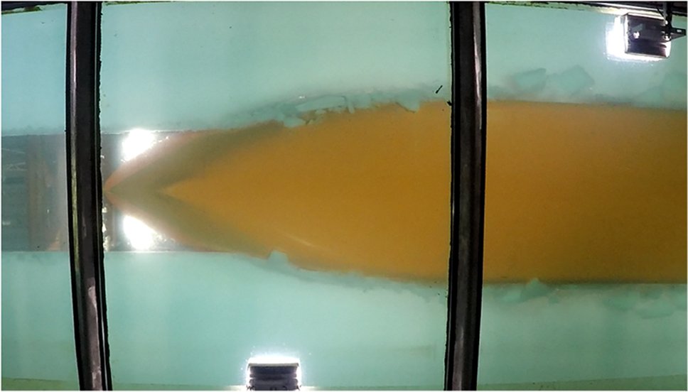 Figure 4 Model tests of large carrier ship in the ice channel free from broken ice. Symmetric movement
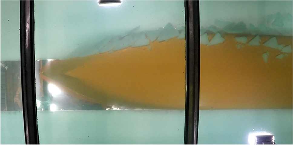 Figure 5 Model tests of large carrier ship in the ice channel free from broken ice. Asymmetric movement
In the case of a symmetrical position, the model's longitudinal central plane coincides with the central axis of the channel.
The model's asymmetrical position was found only in self-propulsion tests when the ice resistance was not measured.
On the basis of visual observations (Figures 4 and 5) from bottom windows, it can be asserted that the theoretical methods suggested for the estimation of broken and level ice resistance components are valid. In particular, the ice edges in both cases (symmetric and asymmetric movement) are broken by bending. Therefore, Ionov's method suggested that for calculation of the respective ice resistance components, $ R_{mI} $ is quite correct.
4.2 Results of Ice Model Tests
Ice resistance of this ship was calculated as per Eqs. (3)–(8) and compared versus the model test data. The ice model tests were carried out for the case of symmetrical movement of the vessel in the channel. The model tests had two stages:
Symmetrical towing of the ship model in ice-free channel (Figure 4)
Symmetrical towing of the ship model in ice channel filled with ice cakes of concentration 8/10 (Figure 6)
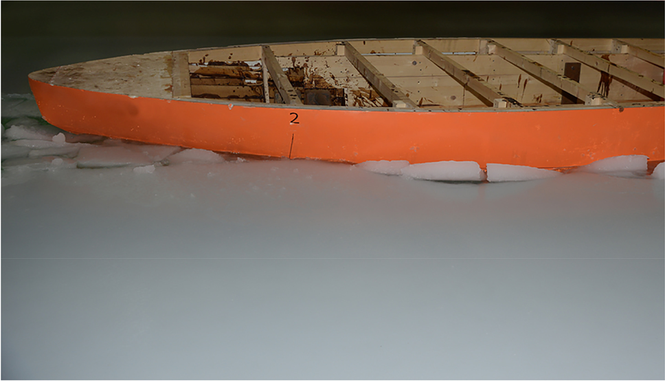 Figure 6 Model tests of large carrier ship in ice channel filled with broken ice. Symmetric movement
At the first stage, the ice edge breaking component was determined. The next stage allowed to determine experimentally the full ice resistance in the channel filled with ice cakes. The difference between the measured results is due to the ice cakes being pushed in the channel by the vessel's hull. The results of this comparison are given in Tables 3 and 4. These data confirm the essential feasibility of ice resistance estimation based on the procedure put forward in this paper.
Table 3 Experimental and calculated ice resistance of carrier ship following an icebreaker in the channel (symmetric movement)Ice thickness (m) Ship speed (kn) Ice resistance, MN Ice edges breaking Ice cakes pushing Total hI V RmI RBIsymm RIsymm 1.5 3.8 1.51 1.26 2.77 1.5 6.3 2.17 1.66 3.83 2.0 3.8 2.59 1.73 4.32 2.0 6.3 3.09 2.40 5.49 Note: Ice model tests results Table 4 Experimental and calculated ice resistance of carrier ship following an icebreaker in the channel (symmetric movement)Ice thickness (m) Ship speed (kn) Ice resistance, MN Ice edges breaking Ice cakes pushing Total hI V RmI RBIsymm RIsymm 1.5 3.8 1.59 1.47 3.06 1.5 6.3 1.85 1.72 3.57 2.0 3.8 2.45 2.01 4.46 2.0 6.3 2.79 2.38 5.17 Note: Calculation results using Eqs. (3)–(8) In addition, the ice resistance was calculated for the asymmetrical pattern of ship motion in the channel. The results are given in Table 5. According to the obtained data, the ice resistance of a ship in the case of asymmetrical motion in the channel increases as compared with the case of symmetrical motion. There is no model experiment confirmation because asymmetrical motion in the channel behind an icebreaker was found only in self-propulsion tests.
Table 5 Experimental and calculated ice resistance of carrier ship following an icebreaker in the channel (asymmetric movement)Ice thickness (m) Ship speed (kn) Ice resistance, MN Ice edges breaking Ice cakes pushing Total hI V RmI RBIasymm RIasymm 1.5 3.8 1.82 1.61 3.43 1.5 6.3 2.34 1.94 4.28 2.0 3.8 2.69 2.19 4.88 2.0 6.3 3.39 2.67 6.06 Note: Calculation results using Eqs. (3)–(8) It is quite clear that the new procedure for the calculation of ship ice resistance in a narrow channel needs further refinement. The basis of the results of ice model tests and of the comparison performed ways for refinement of the new procedure was determined.
4.3 Ways to Improve the Calculation Method
The Eq. (5) gives a conservative result and needs updating. This equation involves the ice resistance component based on icebreaking by the stem. It could constitute a considerable part of the full ice resistance due to the input data made use of for calculation. This resistance component was considered during the calculations, but this assumption would need to be revisited in the future. No such assumption was made during the ice tests, which makes their results more accurate.
The calculation procedure should consider the fracturing of channel edges. It is a well-known fact that channel making by an icebreaker creates a system of radial and circular fractures. The ice pieces are usually broken at the fracture nearest to the hull (Appolonov et al. 2000). Thus, channel edges broken by the hull of a carrier are more fractured than the intact ice sheet. No such assumption was made during ice tests, too.
It is necessary to update the hydrodynamic resistance data for large carrier operating in ice conditions, especially at speeds above 2–3 m/s (Sazonov and Dobrodeev 2018), because this component of the full ship resistance is relatively unexplored for high-speed movement in ice.
As a result, the suggested approach yields quite a conservative result. But the main idea of this research was to obtain a simple semi-empirical equation which could allow fast assessment of ice resistance in the narrow fresh channel behind an icebreaker, because this is a highly relevant task due to the developing marine transport systems along the North Path Way.
Apparently, the ice edge breaking component of ice resistance could also be determined by means of more complex calculation methods (Lindqvist 1989; Su et al. 2010; 2011; Tan et al. 2014). However, to apply all possible methods, it might be necessary to introduce the updates formulated above.
4.4 Influence of the Breaking Ice Component on the Total Ice Resistance
The model test data and calculation results make it possible to evaluate the effect of broken ice in the channel upon the total resistance of carriers. The data given above show that broken ice may increase the total ice resistance by 40% and, probably, more (Tables 3 and 4). This increase grows with the ship speed and the ice thickness. It can be concluded that large size carriers operating in ice channels may slow down considerably for two reasons:
(1) The necessity to break ice edges of a narrow channel
(2) Broken ice in the channel
The broken ice effect upon the total resistance of a large carrier ship was analysed by means of calculations performed as per Eqs. (3) and (4). The results of this analysis are given in Figures 7, 8, and 9. The solid and dotted curves in these figures denote symmetric and asymmetric movement, respectively.
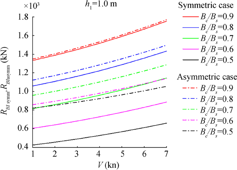 Figure 7 Broken ice resistance of large size carrier moving in the channel. Ice thickness hI = 1.0 m
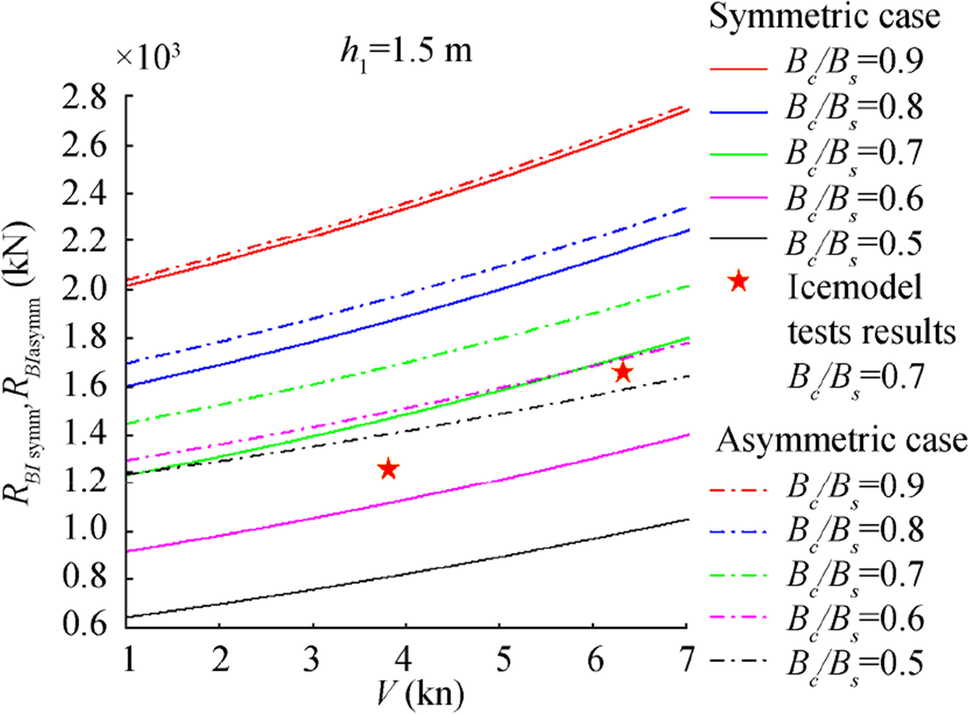 Figure 8 Broken ice resistance of large size carrier moving in the channel. Ice thickness hI = 1.5 m
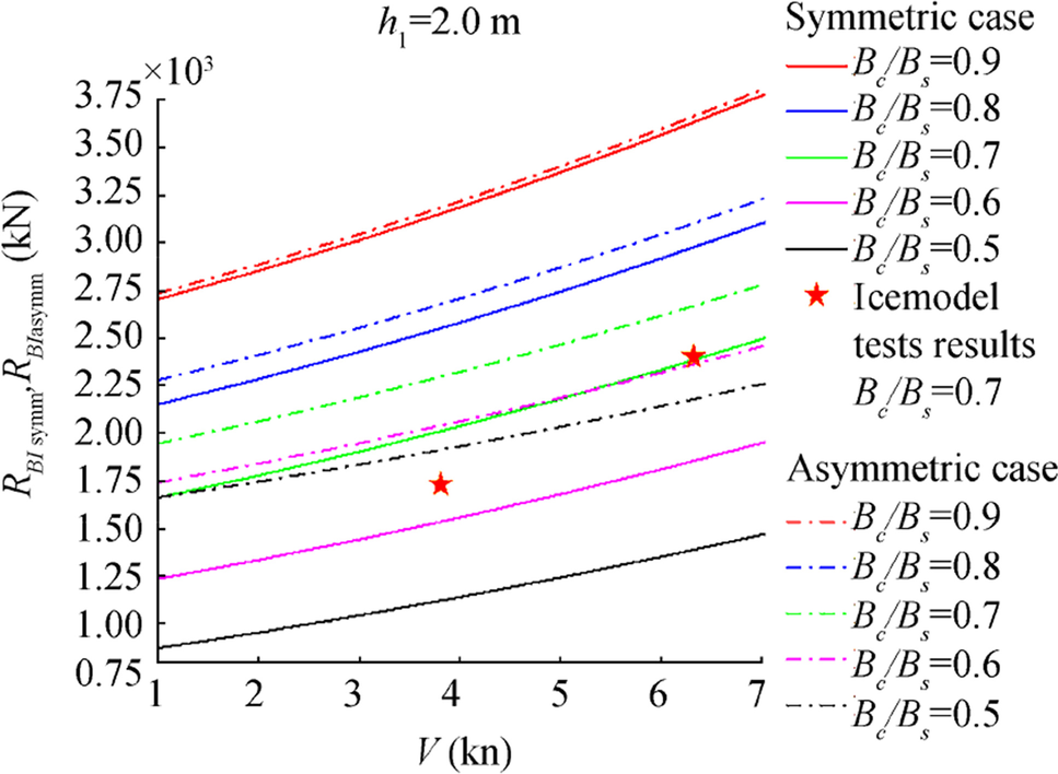 Figure 9 Broken ice resistance of large size carrier moving in the channel. Ice thickness hI = 2.0 m
Analysis of these figures confirms that ice resistance due to the presence of broken ice in the channel depends on the ship speed and ice thickness. This total ice resistance component is different for symmetric and asymmetric movement, the greatest difference taking place in the case of small relative channel widths. When ${}^{{{B}_{C}}}\!\!\diagup\!\!{}_{{{B}_{S}}}\;\to 0$, the difference disappears. Expectedly, the broken ice resistance is greater in the case of asymmetric movement.
5 Conclusions
In this paper, a new method for ice resistance assessment in the case of large size carriers was proposed. It is necessary to apply this method at the ship design stage and during development of the marine transportation system. It allows to define the speed of a carrier moving in a narrow ice channel behind an icebreaker in given ice conditions.
Most likely, the proposed procedure gives quite a conservative result, with the error on the safe side. Still, it needs further refinement, and the main ways of this refinement have been discussed in this paper.
The results of this work clearly demonstrate that broken ice in the channel made by an icebreaker may significantly hinder the speed of large size carriers. The resistance component related to interaction of the hull with broken ice accounts for about 40% of the total resistance. In this connection, it should be noted that there are approaches to rid channels of broken ice, so this resistance component can be reduced, thus raising the large size ship speed. One of the possible ways to resolve this challenge is to equip icebreakers with special ice removal tools that would clear the channel behind them. Another option could be bow optimization of carriers that would reduce their broken ice resistance.
-
Figure 1 A large carrier moving asymmetrically in a narrow ice channel
Figure 2 Movement scenarios of large carrier in ice channel: a $ B_{C} \ge B_{S} $; b $ B_{C} \lt B_{S} $, symmetric movement; c $ B_{C} \lt B_{S} $, asymmetric movement
Figure 3 Relative deviation of experimental data and calculation results obtained as per Eq. (2)
Figure 4 Model tests of large carrier ship in the ice channel free from broken ice. Symmetric movement
Figure 5 Model tests of large carrier ship in the ice channel free from broken ice. Asymmetric movement
Figure 6 Model tests of large carrier ship in ice channel filled with broken ice. Symmetric movement
Figure 7 Broken ice resistance of large size carrier moving in the channel. Ice thickness hI = 1.0 m
Figure 8 Broken ice resistance of large size carrier moving in the channel. Ice thickness hI = 1.5 m
Figure 9 Broken ice resistance of large size carrier moving in the channel. Ice thickness hI = 2.0 m
Table 1 Main particulars of considered vessels
Characteristics Ship 1 Ship 2 Ship 3 Ship 4 Ship 5 Length (m) 299 120 259 75 113 Beam (m) 50 22 35 15.4 24 Stem angle (°) 30 20 20 bulb 60 Waterline entrance (°) 35 40 35 55 45 Ice friction coefficient 0.1 0.1 0.1 0.1 0.1 Table 2 Main parameters of tested large size carrier
Parameter Value Length O.A. (m) 299.0 Beam (m) 50.0 Draught (m) 11.8 Stem angle (°) 30.0 Waterline entrance angle (°) 35.0 Ice friction coefficient 0.10 Table 3 Experimental and calculated ice resistance of carrier ship following an icebreaker in the channel (symmetric movement)
Ice thickness (m) Ship speed (kn) Ice resistance, MN Ice edges breaking Ice cakes pushing Total hI V RmI RBIsymm RIsymm 1.5 3.8 1.51 1.26 2.77 1.5 6.3 2.17 1.66 3.83 2.0 3.8 2.59 1.73 4.32 2.0 6.3 3.09 2.40 5.49 Note: Ice model tests results Table 4 Experimental and calculated ice resistance of carrier ship following an icebreaker in the channel (symmetric movement)
Ice thickness (m) Ship speed (kn) Ice resistance, MN Ice edges breaking Ice cakes pushing Total hI V RmI RBIsymm RIsymm 1.5 3.8 1.59 1.47 3.06 1.5 6.3 1.85 1.72 3.57 2.0 3.8 2.45 2.01 4.46 2.0 6.3 2.79 2.38 5.17 Note: Calculation results using Eqs. (3)–(8) Table 5 Experimental and calculated ice resistance of carrier ship following an icebreaker in the channel (asymmetric movement)
Ice thickness (m) Ship speed (kn) Ice resistance, MN Ice edges breaking Ice cakes pushing Total hI V RmI RBIasymm RIasymm 1.5 3.8 1.82 1.61 3.43 1.5 6.3 2.34 1.94 4.28 2.0 3.8 2.69 2.19 4.88 2.0 6.3 3.39 2.67 6.06 Note: Calculation results using Eqs. (3)–(8) -
Appolonov EM, Nesterov AB, Sazonov KE (2000) Ensuring ice qualities for large capacity arctic tankers. In: Proceedings of the 6th international conference on ships and marine structures in cold regions. St. Petersburg, Russia, pp 64–70 Backstrom M, Juumma K, Wilkman G (1995) New icebreaking tanker concept for the Arctic (DAT). In: Proceeding of the 13th port and ocean engineering under arctic conditions. Murmansk, Russia. Dobrodeev AA (2018a) Refinement of approaches to estimation of ship ice resistance in ice channel based on data from physical model experiments. In: Proceedings of the 37th international conference on ocean, offshore & arctic engineering. Madrid, Spain, OMAE2018–77396 Dobrodeev AA, Klementyeva NY, Sazonov KE (2018) Large ship motion mechanics in "narrow" ice channel. IOP Conf Ser 193: 012017. https://doi.org/10.1088/1755-1315/193/1/012017 Dobrodeev AA, Sazonov KE (2018) Fast sailing in ice – the new goal of model studies. Naval Arch 1: 22–24 Erceg S, Ehlers S (2017) Semi-empirical level ice resistance prediction methods. Ship Technol Res 64(1): 1–14. https://doi.org/10.1080/09377255.2016.1277839 Ionov BP (1988) Ice resistance and its components. Gidrometeoizadt, Leningrad ((in Russian)) International Towing Tank Conference, Recommended Procedures and Guidelines, 2017. Propulsions tests in ice, 7.5-02-04-02.2. Juva M, Riska K (2002) On the power requirement in the Finnish-Swedish ice class rules. Research report No. 53. Helsinki University of Technology, Ship Laboratory, Winter Navigation Research Board, Espoo Kashtleyan VI, Ryvlin AYA, Fadeev OV, Yagodkin VYA (1972) Icebreakers. Sudostroenie, Leningrad ((in Russian)) Kwok R (2018) Arctic sea ice thickness, volume, and multiyear ice coverage: losses and coupled variability (1958–2018). IOP Sci 13(10): 105005 Lindqvist G (1989) A straightforward method for calculation of ice resistance of ships. In: Proceeding of the 10th port and ocean engineering under arctic conditions. Luleå, Sweden, pp 722–735 Myland D, Ehlers S (2019a) Investigation on semi-empirical coefficients and exponents of a resistance prediction method for ships sailing ahead in level ice. Ships Offshore Struct 14(sup1): 161–170. https://doi.org/10.1080/17445302.2018.1564535 Myland D, Ehlers S (2019b) Model scale investigation of aspects influencing the ice resistance of ships sailing ahead in level ice. Ship Technol Res 67(1): 26–36. https://doi.org/10.1080/09377255.2019.1576390 Sazonov KE, Dobrodeev AA (2014) Different technologies for making a wider channel in ice for large size ships. In: Proceedings of the 24th international offshore and polar engineering conference ISOPE, Busan, South Korea, pp 1171–1176 Sazonov KE, Dobrodeev AA (2018) Challenges of speedy icebreaker-assisted operation of heavy-tonnage vessels in ice. In: Proceedings of the 37th international conference on ocean, offshore & arctic engineering, Madrid, Spain Su B, Riska K, Moan T (2010) A numerical method for the prediction of ship performance in level ice. J Cold Region Sci Technol 60: 177–188. https://doi.org/10.1016/j.coldregions.2009.11.006 Su B, Riska K, Moan T (2011) Numerical simulation of local ice loads in uniform and randomly varying ice conditions. J Cold Region Sci Technol 65(2): 145–159. https://doi.org/10.1016/j.coldregions.2010.10.004 Tan X, Riska K, Moan T (2014) Effect of dynamic bending of level ice on ship's continuous-mode icebreaking. J Cold Region Sci Technol 106–107: 82–95. https://doi.org/10.1016/j.coldregions.2014.06.011 Timofeev OYA, Sazonov KE, Dobrodeev AA (2015) New ice basin of the Krylov State Research Centre. In: Proceedings of the 22nd international conference on port and ocean engineering under arctic conditions, Trondheim, Norway Wilkman G, Juurmaa K, Mattsson T, Laapio J, Fagerström B (2004) Full scale experience of double acting tankers (DAT) Mastera and Tempera. Proceedings of the 17th international symposium on ice, 1, St. Petersburg, Russia, pp 488–497 Zuev VA (1986) Means for extending in-land water navigation period. Sudostroenie, Leningrad ((in Russian))