Mooring Damage Identification of Floating Wind Turbine Using a Non-Probabilistic Approach Under Different Environmental Conditions
https://doi.org/10.1007/s11804-020-00187-7
-
Abstract
This paper discusses the damage identification in the mooring line system of a floating wind turbine (FWT) exposed to various environmental loads. The proposed method incorporates a non-probabilistic method into artificial neural networks (ANNs). The non-probabilistic method is used to overcome the problem of uncertainties. For this purpose, the interval analysis method is used to calculate the lower and upper bounds of ANNs input data. This data contains some of the natural frequencies utilized to train two different ANNs and predict the output data which is the interval bounds of mooring line stiffness. Additionally, in order to reduce computational time and more importantly, identify damage in various conditions, the proposed method is trained using constant loads (CL) case (deterministic loads, including constant wind speed and airy wave model) and is tested using random loads (RL) case (including Kaimal wind model and JONSWAP wave theory). The superiority of this method is assessed by applying the deterministic method for damage identification. The results demonstrate that the proposed non-probabilistic method identifies the location and severity of damage more accurately compared to a deterministic one. This superiority is getting more remarkable as the difference in uncertainty levels between training and testing data is increasing.Article Highlights• The proposed method incorporates a non-probabilistic method into artificial neural network;• The method is trained using constant loads and is tested using random loads.• A non-probabilistic approach is proposed to identify damage in the mooring line system of a floating wind turbine; -
1 Introduction
During the last few decades, due to global warming and environmental pollution, the demand for renewable and clean energy has increased. Wind energy is one of the most progressive renewable energy resources. Hence, it is crucial to develop efficient exploitation tools and improve technologies. In this regard, the application of offshore wind turbines in deeper water is taken into consideration to access higher annual mean wind velocity with less turbulence intensity as well as reducing environmental pollution (Jonkman 2007).
However, as the application of offshore wind turbines tends towards deeper water, the costs of operation and maintenance of floating wind turbines (FWTs) increase (Ciang et al. 2008; Tavner 2012). As a result of this, there is a growing need for monitoring FWT health conditions in order to decrease downtime of FWT and minimize related costs. The existence of damage in FWT components can change the whole FWT response. There are some studies about the effects of failure in FWT components such as blade pitch control system faults, grid loss, and malfunction of the blade (Jiang et al. 2014; Bae and Kim 2015; Etemaddar et al. 2016). Mooring lines system is a significant component of floating structures such as marine vessels, floating production, storage, and offloading (FPSO) and FWT. In the case of faults in the mooring line system in FWT, Bae et al. (2017) studied changes in FWT performance while one of the three mooring lines was intentionally disconnected from the OC4 DeepCwind semisubmersible platform. This disconnection altered the platform and turbine orientations and the tension forces of the remaining mooring lines. They concluded that the mentioned damage could be a significant risk to neighboring FWTs within the range of 700-meter distance. Consequently, accurate and prompt damage detection methods can improve efficiency and protect FWT from various failures.
Damage identification in FWT could be very challenging work because of non-linearity in FWT modeling and existing uncertainties. Uncertainties refer to the inaccuracy of physical parameters, soil-structure interaction, wave load determination, and the theory of wave simulation (Negro et al. 2014). These uncertainties can be divided into two following sets: aleatory and epistemic (Paté-Cornell 1996; Faber 2005). The first type of uncertainty, aleatory uncertainty, is induced by the stochastic nature of the wind and wave loading, which consists of both long-term variation related to temporal weather changes and the short-term variation of wave elevation and wind gusts. The second one, epistemic or model uncertainty, is corresponding to the physical model of environmental processes (Uzunoglu and Guedes Soares 2018; Horn et al. 2019). There have been several studies to consider the effects of uncertainties on the reliability of FWTs. For example, uncertainties associated with applied loads and material properties of structures have been studied in references Hsu et al. (2014), Uzunoglu and Guedes Soares (2018), Horn et al. (2019), Raed et al. (2020), and Slot et al. (2020). Some other studies have evaluated the uncertainties in the soil-structure interaction model and soil properties (Vahdatirad et al. 2013; Carswell et al. 2015; Haldar et al. 2018).
In order to alleviate the effects of uncertainties in structural health monitoring (SHM) two types of damage identification methods have been presented: the conventional probabilistic method and the non-probabilistic method. Several probabilistic studies have been performed on FWT with a concentration on reliability based design optimization (Sørensen and Toft 2010; Andersen et al. 2012; Yang et al. 2015; Mardfekri and Gardoni 2015). For instance, Velarde et al. (2019) developed a probabilistic analysis of offshore wind turbines under extreme resonant response during parked situations. In this study, the probability of failure and annual reliability index were used to carry out a reliability analysis of failure due to bending of tubular in monopile and tower. Malik and Mishra (2015) used four probabilistic neural network models to diagnose the wind turbines faults due to imbalance conditions. The results demonstrated that the probabilistic neural network can detect faults with higher accuracy than previous methods. The efficiency of the probabilistic method to handle uncertainty effects was also proven in other studies (Lee et al. 2005; Bakhary et al. 2007). However, this method has some significant problems such as its assumption of uncertain parameters as normally distributed random variables and insufficient data in experimental studies. In comparison with probabilistic damage detection, the non-probabilistic method does not require any assumption about uncertainties distribution. Furthermore, by applying the non-probabilistic approach, the computation becomes simpler and insufficient data in experimental studies cannot weaken the performance of damage detection method in comparison with the probabilistic method (Padil et al. 2017).
Some studies have been done about damage detection in different components of FWT. For instance, Bi et al. (2017) proposed a new pitch fault detection using a performance curve based on normal behavior models. The results showed that malfunction could be detected by the proposed method earlier than the previous approaches. In addition, identification of damage corresponding to malfunctions in some components such as yaw error and reduction of stiffness related to tower base has been done in reference Avendaño-Valencia and Fassois (2017). In the case of mooring line damage detection, there have been done various studies. For instance, in platforms for offshore oil and gas exploitation, some research has been carried out (Fang and Blanke 2011; Blanke et al. 2012; Ren et al. 2015; Hassani et al. 2017; Rezaniaiee Aqdam et al. 2018, b). Particularly in FWT, Jamalkia et al. (2016) applied a fuzzy-based damage detection method using the dynamic response of the FWT structure to identify FWT mooring lines damages. The simulation results illustrated that the proposed method is able to identify damage classes with and without weak noise. Nevertheless, there are some drawbacks in using fuzzy classification in high damage severities as described in reference Ettefagh and Sadeghi (2008). In this method, the weighting parameters are chosen by expert knowledge. Therefore, the results of damage detection could be affected by the value of these parameters. Another problem of the mentioned study is that damage detection was carried out in some classes while it could be more accurate if the damage detection method identifies the exact proportion of damage or stiffness of mooring lines. This study also used CL case to simulate environmental conditions due to high computational cost for exact modeling by applying RL case.
In order to overcome the abovementioned drawbacks, a new damage detection method is presented based on the non-probabilistic method. For this purpose, the method is trained, using the features related to CL case. However, the RL case is utilized for testing the method. Hence, the proposed method can be robust with respect to different environmental conditions and uncertainties. Additionally, this method decreases computation complexity by using consistent environmental conditions for training data. It should be added that while damages are occurring in different types, some of the natural frequencies are shifting. The relationship between these frequencies and damage types is not linear. Therefore, in this study, the ANN method is used to identify damage types since it enables to establish a non-linear relationship between inputs and outputs. ANNs have been widely utilized in FWT (see, e.g., refs. Wen et al. 2019; Asgharnia et al. 2020; Sessarego et al. 2020 for design optimization and refs. Kim et al. 2018; Li et al. 2018; Rezaniaiee Aqdam et al. 2018; Qiu et al. 2020 for fault detection). In reference Marugán et al. (2018), a review study has been performed on the application of ANN for various purposes in the wind energy system, which is insightful for new readers.
The rest of the paper is structured as follows: Dynamic FWT simulations corresponding to different environmental conditions are firstly discussed in Section 2. The effect of mooring line damage on dynamic response and feature selection are studied in Section 3. The application of the non-probabilistic ANN method for damage detection is described in Section 4. Finally, damage identification results and conclusion sections are respectively explained in Sections 5 and 6.
2 FWT Dynamic Simulations in Different Environmental Conditions
The FWT model that is suggested by Wang and Sweetman (2012) and applied in our previous studies (Jamalkia et al. 2016; Jahangiri and Ettefagh 2018) is used in this research to simulate the behavior of FWT. This model considers FWT as two rigid bodies including tower platform assembly (TPA) and rotor nacelle assembly (RNA). The function of this model is completely suited to the purpose of this research to identify different damage types in mooring lines of FWT with respect to different environmental conditions. As these damage types cause the large amplitude of FWT response, it is necessary that the model of FWT should be capable to simulate large rotations. It should be noted that the suggested model by Wang and Sweetman (Wang and Sweetman 2012) can accomplish this need by using several different coordinate systems. In order to calculate the large-amplitude rotation of tower, from 12 possible Euler angles sequences, 1-2-3 sequence Euler angles X4, X5, and X6 are used. A schematic of the FWT and its DOFs, coordinate systems, and module of mooring lines with respect to wave and wind directions are respectively illustrated in Figure 1a, b, and c.
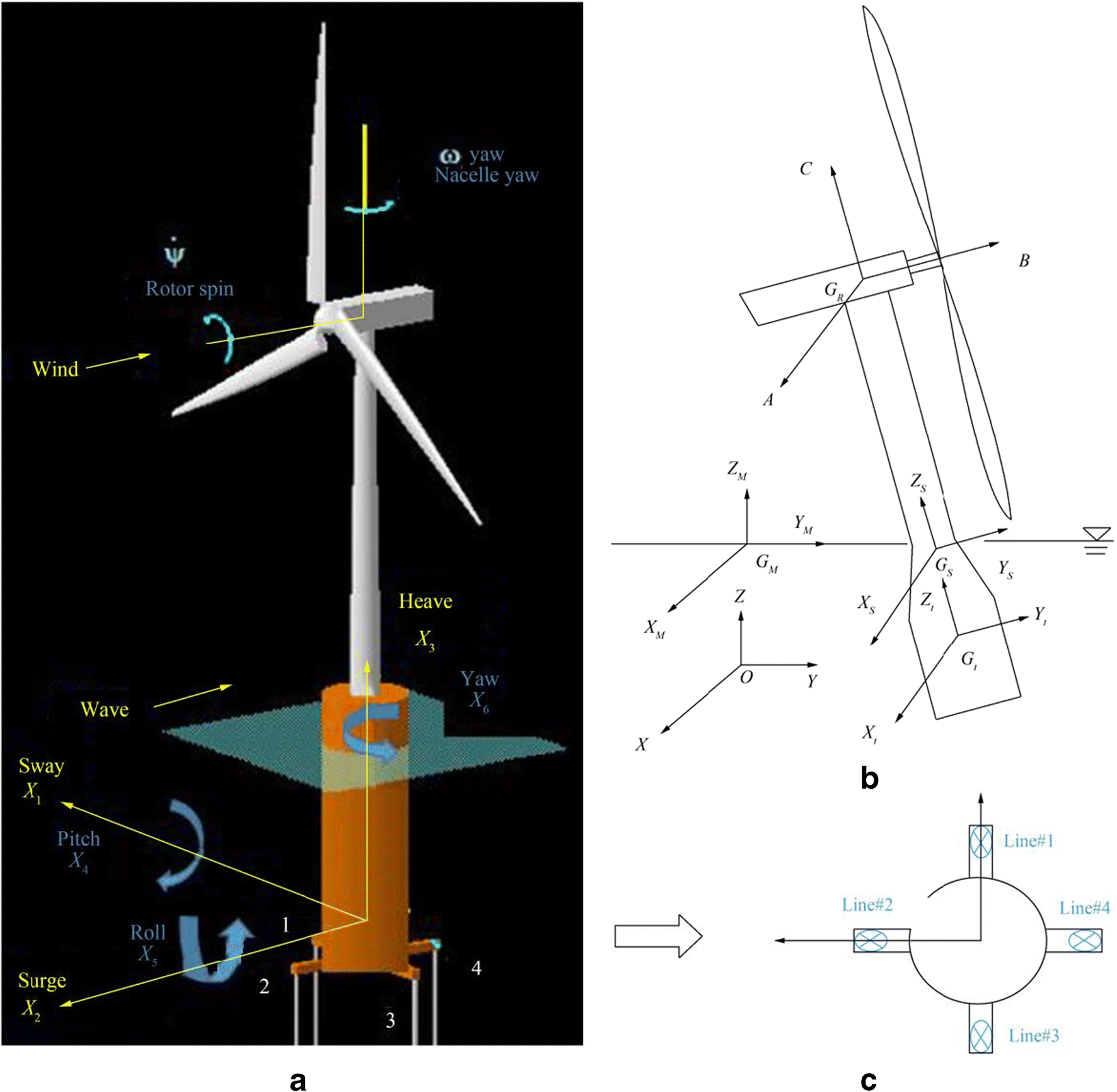 Figure 1 FWT specifications. a A schematic of FWT and its DOFs. b Coordinate systems used in modeling of FWT (Wang and Sweetman 2012). c An illustration of mooring lines with respect to wave and wind directions
As it is shown in Figure 1b, several coordinate systems, including (xt, yt, zt), (A, B, C), and (xs, ys, zs), are respectively used to indicate the coordination of TPA, RNA, and multi-body system. Also, Gt, GR, and GS demonstrate the center mass (CM) of the mentioned coordinate systems respectively. With respect to Figure 1c, it is clear that the directions of wave and wind are in the opposite direction of surge motion. The external loads including the hydrostatic, wind, wave, and mooring lines are calculated based on reference Wang and Sweetman (2012).
2.1 Generation of Wind and Wave Time Series
Wind and wave are two main factors, which affect FWT's whole response. To obtain a realistic response for FWT, a stochastic wave model and a turbulence wind model are required. For this purpose, the Kaimal spectrum is used to generate turbulent wind speed. The mean wind velocity and parameters of the spectrum are chosen corresponding to the FWT condition based on reference Dyrbye and Hansen (1997). Furthermore, a JONSWAP spectrum is applied to simulate the wave. In addition, the correlation between mean wind speed and sea condition should be regarded for realistic simulation of environmental conditions. A joint probability density distribution of the characteristic parameters such as the significant wave height, Hs, the mean wind, Vm, and spectral peak period of the wave, Tp, is needed (Johannessen et al. 2002). Environmental data from reference Jiang et al. (2014) are used hereafter with values of Vm = 8 m/s, Hs = 2.5 m, and Tp = 9.9 s. Other parameters of the JONSWAP spectrum such as a peak enhancement factor and peak-shape parameter are calculated based on the IEC 61400-3 design standard (International Electrotechnical Commission (IEC) 2009). The simulation wind speed is shown in Figure 2a. Also, Figure 2b illustrates the Kaimal spectrum and the corresponding spectrum calculated from the simulated time series of wind speed. Similarly, in Figure 3a and b, simulation wave elevation, and corresponding JONSWAP spectrums are respectively shown.
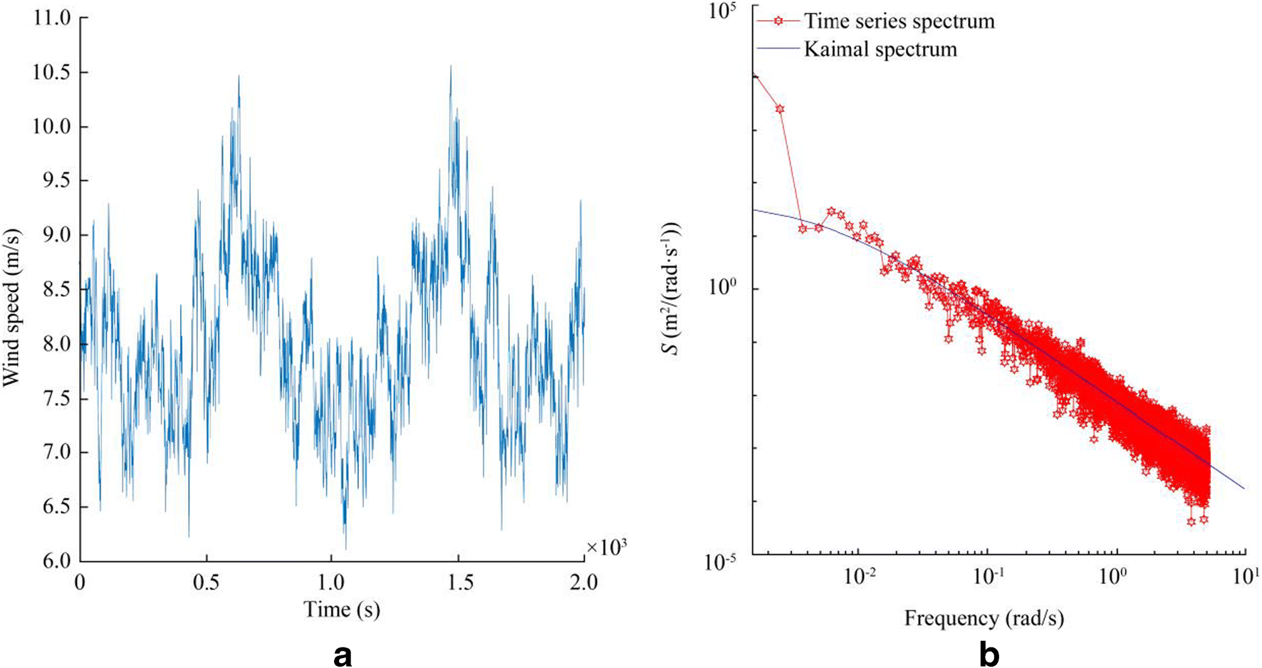 Figure 2 Simulation of the Kaimal spectrum. a Wind time series generated from the Kaimal spectrum for 2000 s. b Comparison between the Kaimal spectrum and time series spectrum
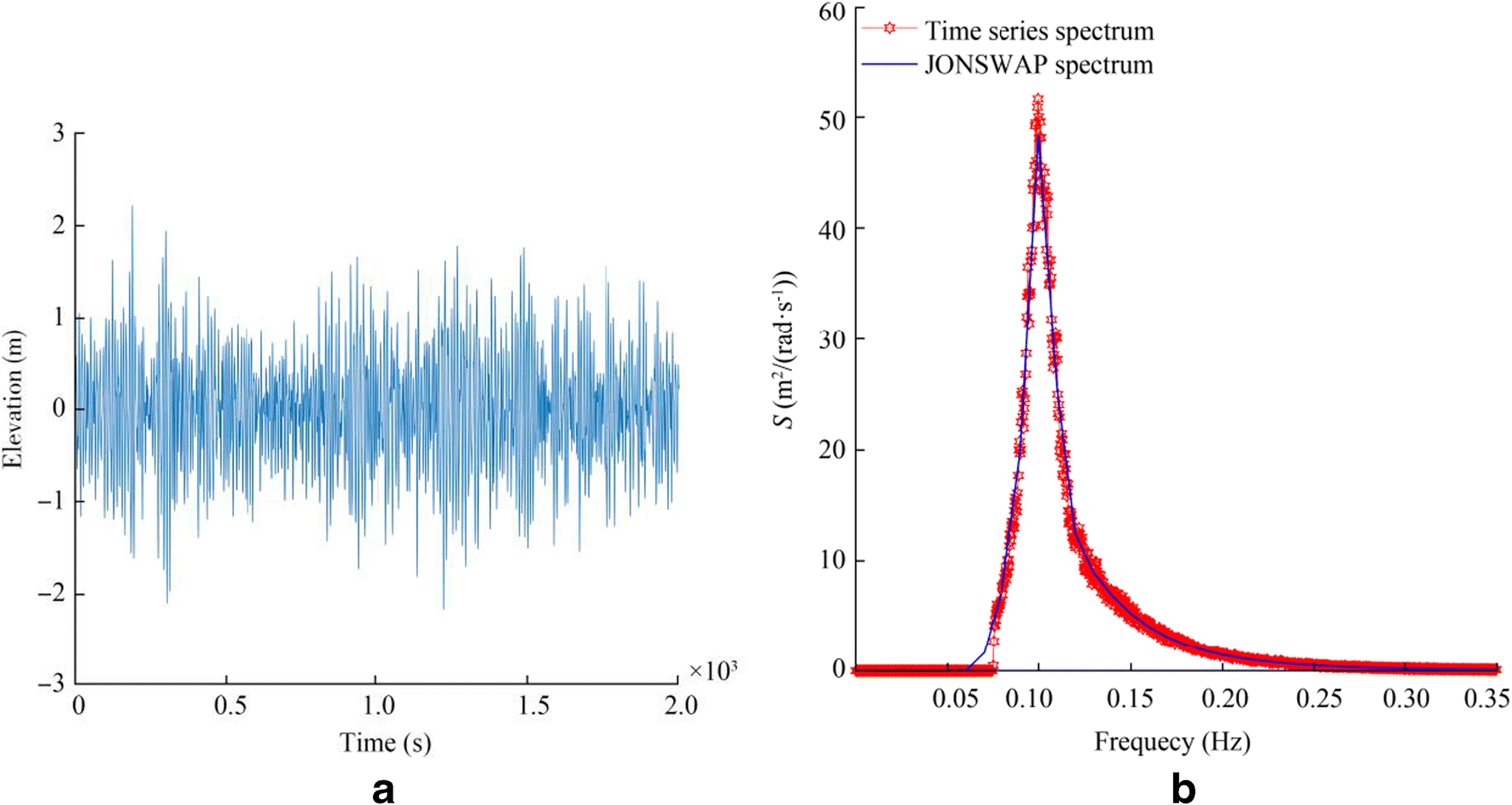 Figure 3 Simulation of the JONSWAP spectrum. a Wave elevation, generated by the JONSWAP spectrum for 2000 s. b Comparison between the JONSWAP spectrum and time series spectrum
As it is obvious from Figures 2 and 3, the wind and wave spectrum, generated by time series, match with corresponding Kaimal and JONSWAP spectrum, respectively.
2.2 FWT Dynamic Results
In order to obtain platform response, equations of motion (EOMs) must be extracted and solved by numerical methods. In this regard, EOMs were derived using Euler-Newton laws. The first EOM is obtained to reach translational responses using Newton's second law and the second one is solved to reach the rotational DOFs using conservation of angular momentum. These EOMs are extended in detail in reference Wang and Sweetman (2012). Platform and tower specifications of NREL 5 MW from reference Matha (2010) are considered a case study for analyzing the proposed damage detection method. For FWT simulation in various environmental conditions, two load cases (constant and random) are applied in wind and wave generation. A constant wind velocity (Vm = 8 m/s) and regular airy wave are considered "constant load (CL)" case. To generate "random load (RL)" case, Kaimal spectrum is used to generate turbulent wind speed with the same mentioned mean wind velocity. In addition, JONSWAP irregular wave theory is used for random wave generation with the same significant wave height and dominant wave period (Hs = 2.5 m and Tp = 9.9 s). The effects of changing CL case to RL ones on FWT responses are illustrated in Figure 4.
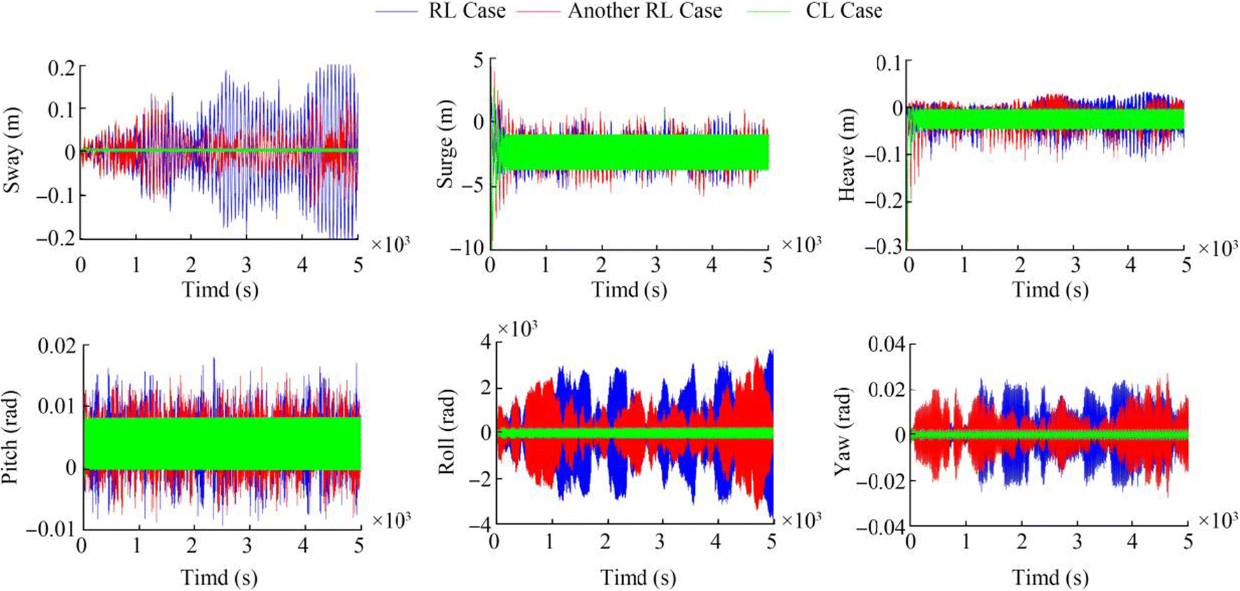 Figure 4 Comparison of FWT response with respect to different loading conditions
Figure 4 shows changing environment conditions from CL to RL cause considerable differences in the response specifications such as mean value and standard deviation. In addition, different types of RL cases produce distinctive responses, which is expected because of the stochastic nature of the applied loads in each RL case. As it can be observed from Figure 4, the surge response fluctuates in negative range and pitch motion has a positive mean. Also, the surge and pitch responses have a bigger standard deviation compared to the sway and roll ones. These results are expected because wave and wind directions are the opposite direction of surge one. Also, the negative mean of the heave response is caused by the mooring line forces.
3 Damage Description and Features Selection
In this study, one of the stiffness of mooring lines is assumed to be reduced while the others are undamaged. There are 1067 damaged and undamaged simulations which are divided into 85%, and 15% used for training and testing ANNs, respectively. The data is related to training ANNs, in turn, is divided into the following sets: 67% for training data and 33% for validation data, which enable applying early stopping criteria (Prechelt, 1998). It should be added that among this data, 907 simulations are carried out by using CL case and used for training data and validation data. The remaining data, 160 cases, is corresponding to RL case and used for testing ANNs. The damages are simulated by randomly stiffness reduction from 1 to 80 percent (with uniform PDF) in each of the mooring lines. It could be explained that FWT with respect to one broken mooring line in TLP remains hydrostatically stable in spite of OC4 DeepCwind semisubmersible (Bae et al., 2017) and this range of stiffness reduction is selected to detect damage in advance of the broken mooring lines. It should be added that in each damage simulation in RL case, distinctive wave condition and wind speed are used to actualize realistic conditions. The effects of stiffness reduction of mooring lines on PSD of the FWT responses in RL cases are illustrated in Figure 5. It should be noted that in the recent figure, one undamaged simulation and two damaged simulations corresponding to each of mooring Line #3 and #4 with damage severity level 40% are carried out.
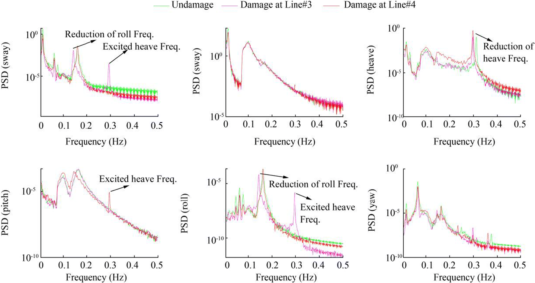 Figure 5 PSD comparison of FWT response with respect to different undamaged and damaged conditions
As it is obvious from Figure 5, some of the natural frequencies are displacing with respect to damage location (mooring line number) and severity (amount of mooring stiffness reduction in the corresponding location). The first example can be related to heave PSD. In this case, when the stiffness of mooring Line #3 or #4 is reduced, the location of heave natural frequency changed. For the second example in the PSDs of sway and roll, when damage exists in Line #3, the roll natural frequency is shifting. However, this frequency is fixed when the damage occurs at Line #4. The values of the mentioned frequencies are decreasing while the severity of damage is increasing. This phenomenon is predicted because when the severity of damage is increasing, the value of the equivalent stiffness of the system is reducing. As it is expected, when damage is occurring at Line #3, the PSDs of sway and roll motions are changing (reduction of roll frequency and excited heave frequency). Because the Line #3 is along with the sway axis, any reduction of its stiffness will change their restoring force and corresponding motions (sway and roll). Another interesting phenomenon is that some of the damage types can excite some of the natural frequencies in some PSDs. For instance, when damage is in Line #3, heave frequency in roll and sway PSDs can be excited and displacing with regard to damage severity; however, when damage exists in Line #4, this natural frequency is not found in these PSDs. As it was mentioned in the introduction, one of the main contributions of this paper is that features which are associated with CL and different RL cases are used for training and testing of the damage detection method, respectively. Therefore, the features should be selected so that they are robust to the environmental conditions. For this purpose, statistical features such as Root Mean Square, standard deviation, Kurtosis, and shape factor are not applicable to damage detection as it is obvious from Figure 4. On the one hand, damages alter the mentioned statistical features and energy of the signal. On the other hand, changing the environment condition from CL to RL case and different RL cases (environment conditions) have more influence on statistical features. Thus, damage detection should employ some features that would proceed damage location and severity whereas they are almost constant with environmental variations. In this regard, as it was shown and discussed in Figure 5, the positions of dominant roll frequency in PSD of roll or sway response (Fe#1) and heave natural frequency in PSD of heave response (Fe#2) are selected as input features. It should be added that except for the mentioned features, other dominant frequencies are not used for damage detection. Because these frequencies are constant during various damage types. It can be mentioned when damage occurs in mooring Line #1 or #2, the corresponding features are exactly equal with mooring Line #3 and #4 ones respectively. This equality occurs because the mentioned mooring lines have symmetric locations. Therefore, damage at Line #1 and #3 can be distinguished from damage at Line #2 and #4, while the damage detection method cannot distinguish damage types at Line #1 from Line #3 (or Line #2 from Line #4). In this regard, it is assumed different damage types occur at Line #3 or Line #4 by considering other lines are undamaged.
4 Damage Detection Methodology
To consider the uncertainties of FWT dynamic model, insufficient data, and making proposed damage detection method practical, two approaches can be used: the non-probabilistic and the probabilistic methods. As it was mentioned in the introduction section, the non-probabilistic method is utilized to reduce computational time. In addition, it does not require any assumption about probability density function (PDF) of uncertainties. This advantage of the non-probabilistic method is very important, especially when proper PDFs cannot be estimated for evaluating all effects of uncertainties which are necessary for every damage identification method. The input parameters of the damage detection method are extracted features, as explained in the previous section, and the outputs are the stiffness values of the mooring lines. However, this relationship between the inputs and outputs is not linear. Therefore, the damage detection method must model non-linear relationships. ANNs are wildly applied in pattern recognition and classification field because ANNs have been proven to be an efficient approach for non-linear mapping between input and output (Padil et al., 2017). Hence, ANN is used in this study.
4.1 Non-Probabilistic Method
In contrast with the probabilistic method in which white Gaussian noise with various variances is applied for modeling uncertainties in the damage identification process, interval analysis is used in the non-probabilistic method. For this purpose, the upper and lower bounds of input $ \left({\lambda}_c^I\right) $ are obtained to reach interval bound output $ \left({K}_c^I\right) $ based on reference Padil et al. (2017).
In the first ANN model, as tabulated in Table 1, lower bound of input is obtained by subtracting uncertainty level from corresponding features and in the second ANN, the upper bound of input is defined by adding uncertainty level to associated features (Padil et al., 2017). The lower and upper bounds of input are used to predict the lower and upper bound of network output, respectively.
Table 1 Input and output of ANN models applied in training and testing steps (Padil et al., 2017)Model Training input Testing input Output ANN1 $ \underline {\lambda_{c, i}^{I, r}}={\lambda}_{c, i}^{I, r}-{\lambda}_{c, i}^{I, r}\times \omega $ $ \underline {\lambda_{c, i}^{I, e}}={\lambda}_{c, i}^{I, e}-{\lambda}_{c, i}^{I, e}\times \omega $ $ \underline {K_{cm}} $ ANN2 $ \overline{\lambda_{c, i}^{I, r}}={\lambda}_{c, i}^{I, r}+{\lambda}_{c, i}^{I, r}\times \omega $ $ \overline{\lambda_{c, i}^{I, e}}={\lambda}_{c, i}^{I, e}+{\lambda}_{c, i}^{I, e}\times \omega $ $ \overline{K_{cm}} $ In Table 1, superscripts r and e are respectively used to demonstrate the training and testing data. The variable ω is used to denote the uncertainty level. The number of damage simulation and frequency features are respectively indicated by subscripts c and i. The number of mooring line, in Kcm, is demonstrated with subscript m, which could be related to Line #3 or Line #4. It should be noted that ANN models are trained by lower and upper parameters from CL case data. Then, the lower and upper bounds of inputs, corresponding to RL simulation, are calculated to identify the corresponding damage location and severity in the testing process of ANNs. It should be explained that for training the non-probabilistic method, the variable ω is assumed 2%. This percentage is selected because the training features and testing features have the maximum difference with each other within the range of 2%.
4.2 Damage Index
Three damage indices are used in this research in order to calculate the possibility of existence damage, comparing different damage severity levels with each other, and making identification result as a quantitative measure. The first damage index is used in deterministic ANN. In contrast with the non-probabilistic method, the deterministic method contains one ANN model and is trained without consideration of uncertainties. In this index, the stiffness reduction factor (SRF), is defined as the ratio of the stiffness reduction to the initial stiffness value as follows:
$$ \mathrm{SRF}=\frac{K_u-{K}_d}{K_u} $$ (1) where Ku and Kd indicate undamaged and damage stiffness respectively. In order to identify damage types by proposed Non-probabilistic method, the possibility of damage existence (PoDE) and the damage measure index (DMI) indices suggested respectively by Wang et al. (2008, 2014) and applied by reference Padil et al. (2017), are used. High values of PoDE demonstrate that the occurrence of damage at the specific mooring line is more possible. The PoDE is calculated based on upper and lower bounds of undamaged and damage stiffness as defined in Table 1. Figure 6 shows the illustration of PoDE calculation.
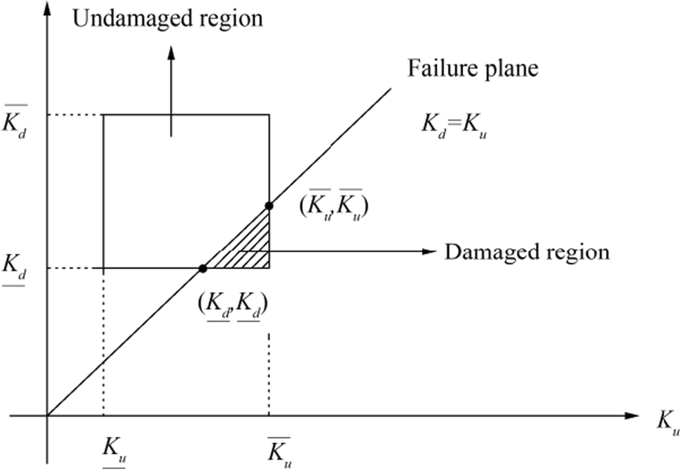 Figure 6 The undamaged and damaged region, which is used for defining PoDE
In Figure 6, the solid rectangle is the region of variation of both damaged and undamaged parameters, which is being crossed by the failure plane $ {K}_u^I={K}_d^I $. It should be mentioned that this figure must be provided for each of the simulation runs and mooring lines. The hatched region is corresponding to the damage region. The undamaged and total areas are associated with the unshaded and solid rectangular region, respectively. Now, the PoDE is defined based on non-probabilistic set-theoretic failure measure as the ratio of damage region area to the area of the total region as follows (Padil et al., 2017):
$$ \mathrm{PoDE}=\frac{A_{\mathrm{damage}}}{A_{\mathrm{total}}} $$ (2) The PoDE values could occur between 0% and 100%. An illustrative example of different PoDE ranges is shown in Figure 7. While the interval bound of damaged stiffness moves toward the interval bound of undamaged stiffness, the PoDE values decrease from 100% to 0%.
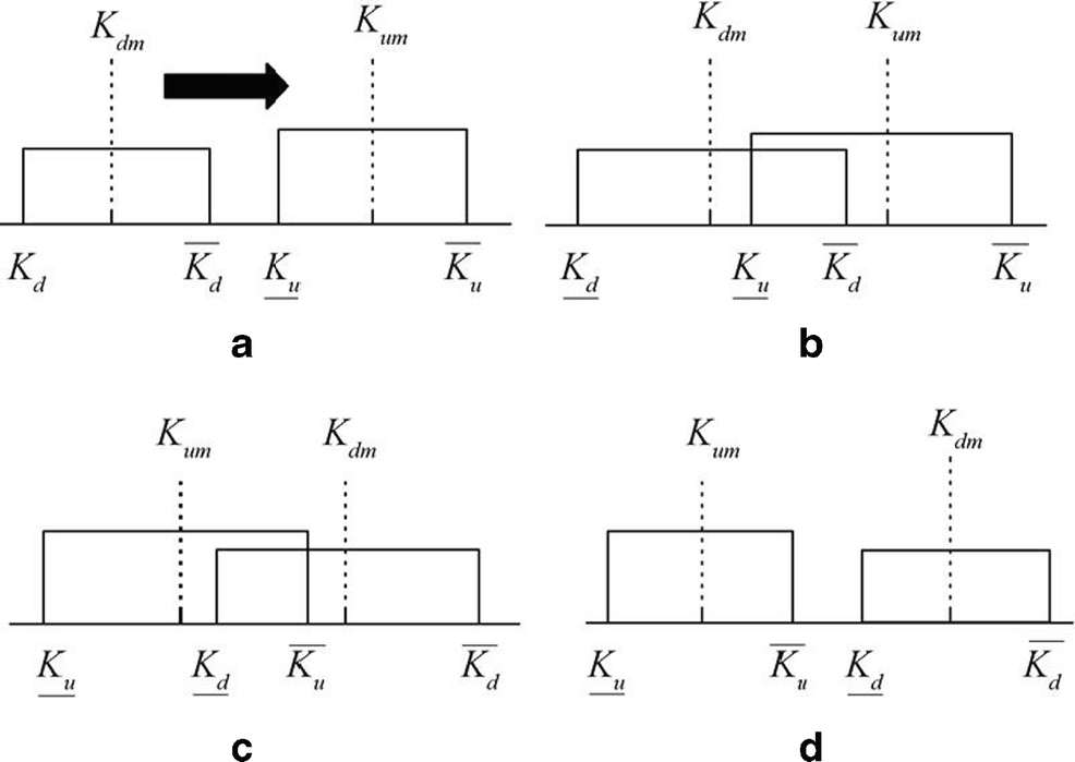 Figure 7 Some illustrative examples of different PoDE ranges
In Figure 7, Kdm and Kum are respectively used to demonstrate the middle values of intervals of $ {K}_u^I $ and $ {K}_d^I $ which are defined as (Padil et al., 2017):
$$ \left\{\begin{array}{l} K_{d m}=\frac{\left(\overline{K_{d}}+\underline{K_{d}}\right)}{2} \\ K_{u m}=\frac{\left(\overline{K_{u}}+\underline{K_{u}}\right)}{2} \end{array}\right. $$ (3) In Figure 7a, the PoDE value is 100% and occurs when the upper bound of damage stiffness is equal or less than the lower bound of undamaged stiffness. Figure 7b and c are related to the conditions that PoDE value is between 0 and 100% and the interference exists between interval bounds of damaged and undamaged parameters. However, the PoDE value corresponding to Figure 7b is bigger than corresponding to c. When the upper bound of undamaged stiffness is equal or less than the lower bound of damaged stiffness, PoDE value is 0% and is plotted in Figure 7d. Therefore, PoDE values for different conditions can be summarized as follows:
$$ \left\{\begin{array}{ll}1,& \overline{K_d}\le \underset{\_}{K_u}\\ {}1-\left(\frac{1/2{\left(\overline{K_d}-\underset{\_}{K_u}\right)}^2}{\left(\overline{K_d}-\underset{\_}{K_d}\right)\left(\overline{K_u}-\underset{\_}{K_u}\right)}\right),& \underset{\_}{K_d} \lt \overline{K_u}\kern0.5em and\begin{array}{cc}& {K}_{dm} \lt {K}_{um}\end{array}\\ {}\left(\frac{1/2{\left(\overline{K_u}-\underset{\_}{K_d}\right)}^2}{\left(\overline{K_d}-\underset{\_}{K_d}\right)\left(\overline{K_u}-\underset{\_}{K_u}\right)}\right),& \underset{\_}{K_d} \lt \overline{K_u}\begin{array}{cc}& and\begin{array}{cc}& {K}_{dm} \gt {K}_{um}\end{array}\end{array}\\ {}0,& \overline{K_u}\le \underset{\_}{K_d}\end{array}\right. $$ (4) The PoDE index is not sufficient to compare different damage and undamaged conditions, because it is a very common situation that in two damage condition with different damage severities, the PoDE values are equal to 100%. In order to overcome this criticism and predict the exact stiffness value, the DMI index is used in this study. The DMI is obtained by multiplying the SRF by the PoDE as follows (Padil et al., 2017):
$$ \mathrm{DMI}=\overline{SRF}\times PoDE $$ (5) where $ \overline{\mathrm{SRF}} $ is calculated by the combination of Eqs. (1) and (3) as follows:
$$ \overline{SRF}=\frac{K_{um}-{K}_{dm}}{K_{um}} $$ (6) The flowchart of damage identification process corresponding to deterministic and non-probabilistic methods is illustrated in Figure 8.
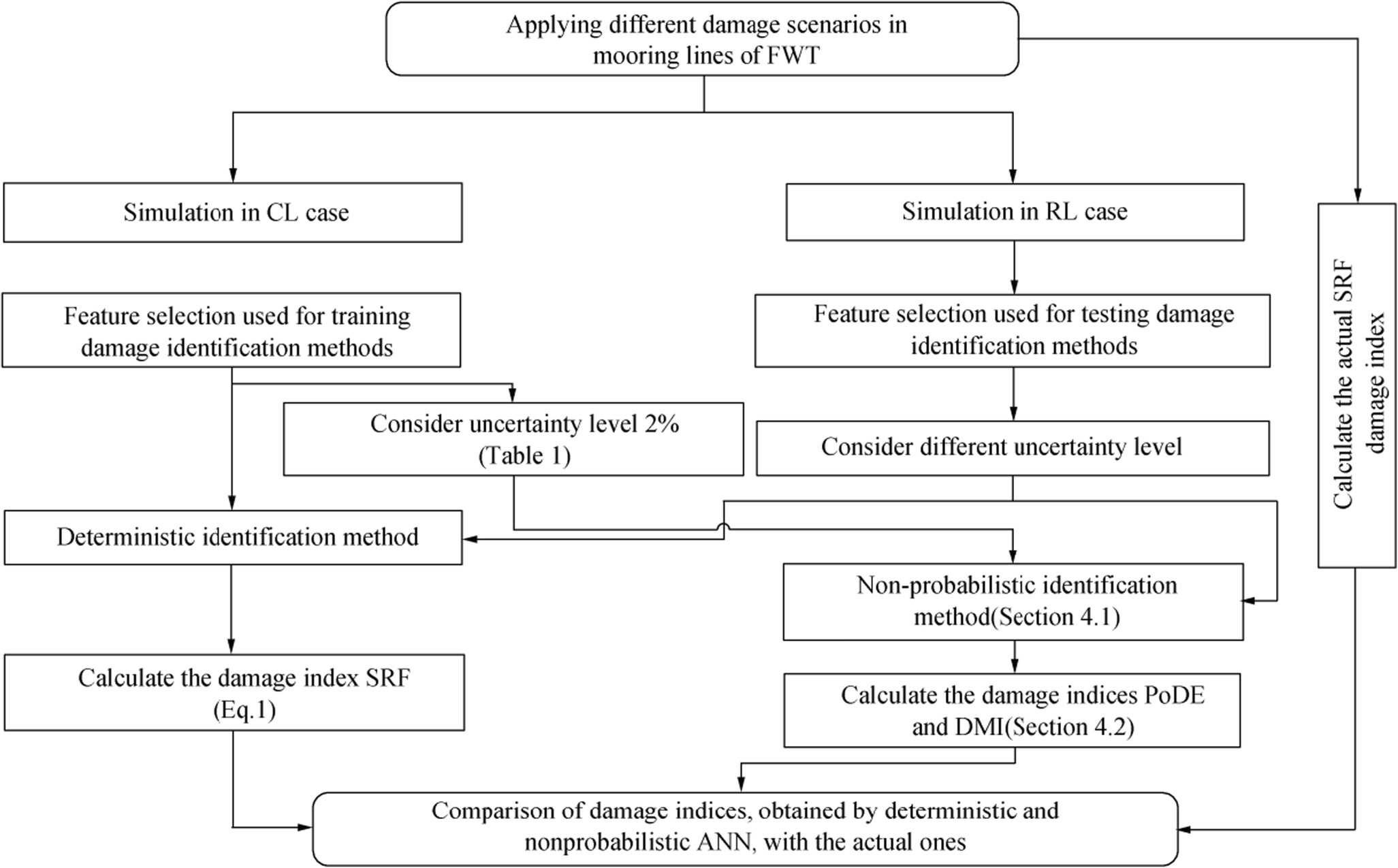 Figure 8 The process of damage identification methods
4.3 Topology of Neural Network
The performance of the neural network in the identification of damage severity and location is related to ANN architecture. The determination of neurons number in the hidden layer of ANN plays a significant role in optimizing the ANN. To illustrate, if the number of neurons is smaller than the optimal value, ANN will not be able to make an accurate relationship between input and output parameters of ANN. On the other hand, if the number of neurons is bigger than the optimal value, ANN will memorize the relationship between inputs and outputs. Consequently, in the cases that uncertainty levels differ between inputs and outputs, ANN cannot predict the outputs values correctly. Therefore, it is critical to determine the number of neurons in the hidden layer, and this determination is conducted by the trial-and-error method. In this study, the influence of neurons number of the hidden layer on ANN prediction error is assessed in Figure 9. In this figure, the value of prediction error in training and validating data are shown.
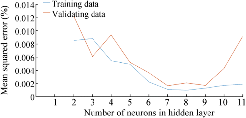 Figure 9 The MSE values of ANN in terms of neurons number in training and validating data
By looking at Figure 9, it is clear that minimum error in both training and validating data occurs when the number of neurons is equal to 7. In addition to the neuron number, transfer function and training algorithm have important impacts on damage identification results. In this research, the log-sigmoid transfer function is selected because the inputs and outputs of ANN are normalized between 0 and 1. Also, the Levenberg-Marquardt training algorithm is utilized to determine the values of weights and biases. The precision and accuracy of this algorithm have been proven in vibration damage identification problems (Lyn Dee et al., 2010). The initial values of weights and biases were generated randomly between − 1 and 1. The early stopping method is used as the training termination point to avoid overfitting problems (Prechelt, 1998). The architecture of ANNs is illustrated in Figure 10, where the inputs of ANNs are roll and heave natural frequencies and the outputs of ANNs are stiffness of mooring Line #3 and Line #4. According to this figure, a number of neurons in the hidden layer and output layer are respectively 7 and 2. As it was mentioned, the number of neurons in the hidden layer was selected by the trial-and-error method. However, the number of neurons in the output layer must be equal to the size of outputs.
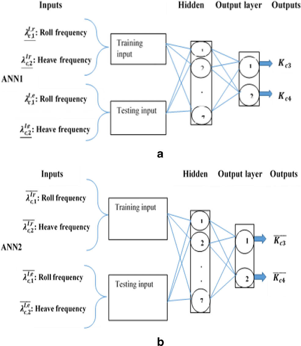 Figure 10 Architecture of multilayer perceptron ANNs. a ANN 1 is used to calculate lower bound of output. b ANN 2 is used to calculate upper bound of output
5 Results and Discussions
In order to assess the deterministic and non-probabilistic methods, 10 damage scenarios are simulated with considering uncertainty level 2%. Five of these scenarios assess damages in the mooring Line #3 by reducing the stiffness of the mooring with 10, 25, 40, 55, and 70 present. Similarly, the rest of the scenarios are introduced with the same stiffness reduction in the mooring Line #4. It should be noted that for consistency and being able to compare the non-probabilistic method with deterministic ones, the architecture and parameters of non-probabilistic ANNs are the same with deterministic ones. Damage identification results including SRF and DMI, are shown in Figure 11. SRF values are corresponding to actual stiffness reduction and deterministic ones. Also, DMI value is calculated through the non-probabilistic method.
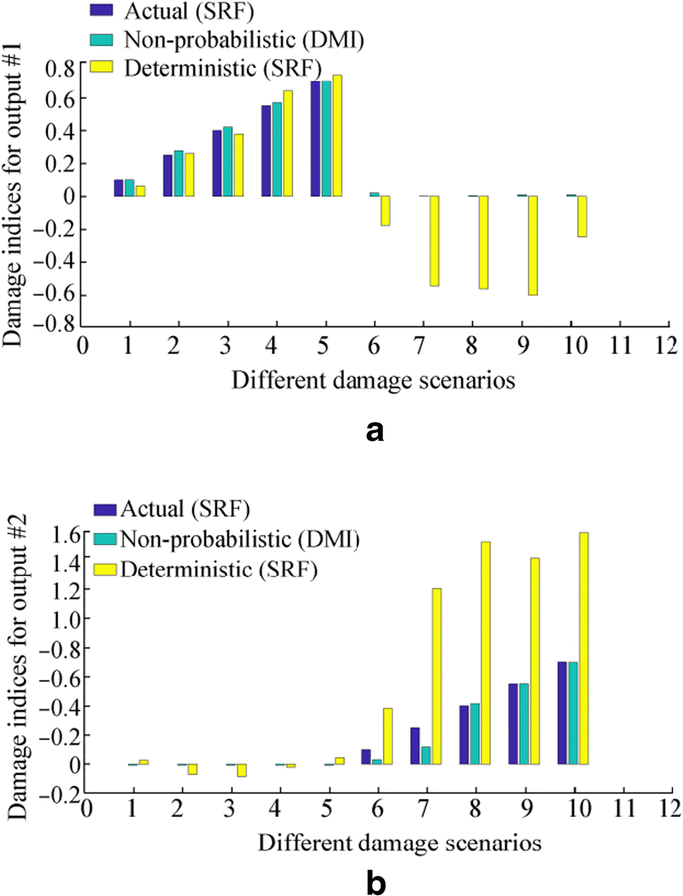 Figure 11 Comparison of damage indices, obtained by deterministic and non-probabilistic ANN, with the actual ones at uncertainty level 2%. a The first output of ANN (corresponding to the stiffness of Line #3). b The second output of ANN (corresponding to the stiffness of Line #4)
Note that the first five of the damage scenarios (1 to 5) are related to the damage in the mooring Line #3 and the second five one (6 to 10) are related to Line #4.
As it is obvious from Figure 11, in most of the damage scenarios, the values of the non-probabilistic DMI index are more close to actual stiffness reduction in comparison with deterministic index especially when the mooring line is undamaged or even light damage occur at mooring lines. For instance, in Figure 11a, deterministic method overestimates stiffness of Line #3 in scenarios #6–10 in which the mooring Line #3 is undamaged. Additionally, in scenario #6 and #7 of Figure 11b, while the actual values of SRF are respectively 10% and 25%, the prediction ones demonstrate 38% and 120%. This common drawback is expectable because the uncertainty level in the deterministic method has more consequences on damage identification when the level of damage is small or in undamaged condition. However, in these mentioned scenarios, the non-probabilistic method has accurate performance.
To investigate the performance of the proposed method in different levels of uncertainties and severities, a profound study is conducted. It should be added that the performance of networks is calculated by mean squared error (MSE) between estimated and real stiffness reduction in three light, medium, and sever types of damages. For this reason, damage types corresponding with 1%–30%, 31%–55%, and 56%–80% stiffness reduction are respectively considered light, medium, and server damages. These categories are applied to compare damage detection methods between different severities. The general results are put in Table 2.
Table 2 Comparison of performance between deterministic and non-probabilistic methods by considering different uncertainty levelsDamage types Mooring Deterministic method (MSE%) Non-probabilistic method (MSE%) Uncertainty level (%) Uncertainty level (%) 1 2 5 7 1 2 5 7 Line #3 (light) 1 0.2158 0.0864 0.729 3.2113 0.1159 0.0053 0.3391 1.4234 2 0.1439 0.0437 30.13 21.596 0.1115 0.0062 0.2439 0.2664 Line #3 (medium) 1 0.0317 0.0966 20.046 135.26 0.0724 0.0349 1.4963 3.6405 2 0.1744 0.72 37.26 13.646 0.1035 0.0064 0.0166 0.2381 Line #3 (severe) 1 0.1095 1.5394 93.944 104.62 0.0537 0.0146 0.6602 3.9508 2 0.4475 0.3206 3.8353 4.7479 0.1429 0.0061 0.0948 0.1126 Line #4 (light) 1 0.5002 7.0255 6.3258 12.231 0.1014 0.0358 0.0421 0.6607 2 0.3668 19.791 60.516 67.606 0.7981 0.5041 0.8004 0.4567 Line #4 (medium) 1 0.7216 30.979 52.233 44.388 0.0923 0.0014 0.0327 0.7391 2 0.5188 110.05 692.14 1104.5 1.0146 0.818 1.5295 10.09 Line #4 (severe) 1 0.1652 25.011 29.454 23.667 0.1543 0.0092 0.099 3.1836 2 1.2151 76.88 582.68 979.69 0.066 0.0041 4.1526 29.496 Total 0.3842 22.712 134.11 209.22 0.2355 0.1205 0.7923 4.5215 It can be seen from Table 2 the deterministic method can identify damage location and severity when the uncertainty level is equal to 1%. In spite of this ability, as the uncertainty level is increasing, the precision of damage identification results is decreasing. For example, as the uncertainty level is rising from 1% to 2 and 5%, the total MSE sharply is increasing from 0.38 to 22.71 and 134.11. The maximum MSE of the deterministic method occurs at 7% uncertainty level.
By looking at the section of the non-probabilistic method in Table 2, some significant results can be drawn: (1) the total MSE values of the non-probabilistic method for uncertainty levels 2%, 5%, and 7% are respectively 0.12, 0.79, and 4.52. These values are entirely smaller than values related to the deterministic method (22.71, 134.11, and 209.22). Therefore, the non-probabilistic method can identify damage types more accurately and reliably. (2) The uncertainty level has also effects on damage identification in the non-probabilistic method. When the difference of uncertainty level in training data and testing data is increasing, the MSE value is raising. For instance, the highest MSE value of the non-probabilistic method (4.52%) is related to uncertainty level 7% case where the difference of uncertainty level between training data and testing data is highest (5%). Moreover, the minimum MSE value corresponds to uncertainty level 2% when the uncertainty level of training and testing data is equal. This behavior could be acceptable; hence, this difference of uncertainty level can significantly reduce the accuracy of the established ANN correlation matrix between inputs and outputs. (3) As for damage types categorized as light, the non-probabilistic method can handle uncertainty effects, even at uncertainty level 7% (with MSE values of 1.42 when damage occurs at Line #3 and 0.66 at Line #4). In contrast, the deterministic method cannot correctly predict the true values of the stiffness of mooring lines (with MSE values 21.596 and 67.6 corresponding to damage at Line #3 and Line #4, respectively). Thus, the ability of the non-probabilistic method to predict light damage can be proven. (4) By drawing a detailed comparison between the result of damage identification when damage occurs at Line #3 and Line #4, it can be concluded the non-probabilistic method and also deterministic one have more prediction error when damage occurs at Line #4 in comparison to Line #3. This interesting difference in prediction error can be related to the features of ANN. As it was mentioned in Section 3, when damage is occurring at Line #3, both features (heave and roll natural frequencies) are changing. Conversely, when damage is taking place at Line #4, individual feature (heave natural frequency) is changing. In other words, the ability of the damage identification methods to predict the stiffness of the mooring line is decreasing while the number of changing feature is reducing. In addition to the mentioned superiority of the non-probabilistic method in terms of accuracy, this method is also required two ANNs, which is fewer in comparison with probabilistic ANNs required four ANNs (Bakhary et al., 2007). Therefore, less computational time is needed to train ANNs in the non-probabilistic method. Additionally, by handling uncertainties, the training of ANNs was carried out with CL case, which needs significantly less computational time to simulation of damaged and undamaged conditions with comparison to RL case.
6 Conclusion
In this study, the existing damages in mooring lines of FWT were identified by two methods as named "deterministic" and "non-probabilistic" based on ANN. Additionally, the comparison was carried out between the mentioned methods. To assess the ability of these methods, the proposed methods are trained with CL case and are tested with RL case. Moreover, several different uncertainty levels are applied to evaluate the influence of uncertainty levels on identification results. These results show that the deterministic method has the ability to predict correctly the location and severity of damage without consideration of the uncertainty level. However, the accuracy of this prediction is getting more false, as the uncertainty level is increasing. In spite of the deterministic method, the proposed non-probabilistic method can handle the problem of uncertainty level, particularly in high uncertainty level (5 and 7%), with the help of its own damage indices, including PoDE and DMI values. Therefore, the identification results of the non-probabilistic method were superiority to deterministic ones.
-
Figure 1 FWT specifications. a A schematic of FWT and its DOFs. b Coordinate systems used in modeling of FWT (Wang and Sweetman 2012). c An illustration of mooring lines with respect to wave and wind directions
Figure 2 Simulation of the Kaimal spectrum. a Wind time series generated from the Kaimal spectrum for 2000 s. b Comparison between the Kaimal spectrum and time series spectrum
Figure 3 Simulation of the JONSWAP spectrum. a Wave elevation, generated by the JONSWAP spectrum for 2000 s. b Comparison between the JONSWAP spectrum and time series spectrum
Figure 4 Comparison of FWT response with respect to different loading conditions
Figure 5 PSD comparison of FWT response with respect to different undamaged and damaged conditions
Figure 6 The undamaged and damaged region, which is used for defining PoDE
Figure 7 Some illustrative examples of different PoDE ranges
Figure 8 The process of damage identification methods
Figure 9 The MSE values of ANN in terms of neurons number in training and validating data
Figure 10 Architecture of multilayer perceptron ANNs. a ANN 1 is used to calculate lower bound of output. b ANN 2 is used to calculate upper bound of output
Figure 11 Comparison of damage indices, obtained by deterministic and non-probabilistic ANN, with the actual ones at uncertainty level 2%. a The first output of ANN (corresponding to the stiffness of Line #3). b The second output of ANN (corresponding to the stiffness of Line #4)
Table 1 Input and output of ANN models applied in training and testing steps (Padil et al., 2017)
Model Training input Testing input Output ANN1 $ \underline {\lambda_{c, i}^{I, r}}={\lambda}_{c, i}^{I, r}-{\lambda}_{c, i}^{I, r}\times \omega $ $ \underline {\lambda_{c, i}^{I, e}}={\lambda}_{c, i}^{I, e}-{\lambda}_{c, i}^{I, e}\times \omega $ $ \underline {K_{cm}} $ ANN2 $ \overline{\lambda_{c, i}^{I, r}}={\lambda}_{c, i}^{I, r}+{\lambda}_{c, i}^{I, r}\times \omega $ $ \overline{\lambda_{c, i}^{I, e}}={\lambda}_{c, i}^{I, e}+{\lambda}_{c, i}^{I, e}\times \omega $ $ \overline{K_{cm}} $ Table 2 Comparison of performance between deterministic and non-probabilistic methods by considering different uncertainty levels
Damage types Mooring Deterministic method (MSE%) Non-probabilistic method (MSE%) Uncertainty level (%) Uncertainty level (%) 1 2 5 7 1 2 5 7 Line #3 (light) 1 0.2158 0.0864 0.729 3.2113 0.1159 0.0053 0.3391 1.4234 2 0.1439 0.0437 30.13 21.596 0.1115 0.0062 0.2439 0.2664 Line #3 (medium) 1 0.0317 0.0966 20.046 135.26 0.0724 0.0349 1.4963 3.6405 2 0.1744 0.72 37.26 13.646 0.1035 0.0064 0.0166 0.2381 Line #3 (severe) 1 0.1095 1.5394 93.944 104.62 0.0537 0.0146 0.6602 3.9508 2 0.4475 0.3206 3.8353 4.7479 0.1429 0.0061 0.0948 0.1126 Line #4 (light) 1 0.5002 7.0255 6.3258 12.231 0.1014 0.0358 0.0421 0.6607 2 0.3668 19.791 60.516 67.606 0.7981 0.5041 0.8004 0.4567 Line #4 (medium) 1 0.7216 30.979 52.233 44.388 0.0923 0.0014 0.0327 0.7391 2 0.5188 110.05 692.14 1104.5 1.0146 0.818 1.5295 10.09 Line #4 (severe) 1 0.1652 25.011 29.454 23.667 0.1543 0.0092 0.099 3.1836 2 1.2151 76.88 582.68 979.69 0.066 0.0041 4.1526 29.496 Total 0.3842 22.712 134.11 209.22 0.2355 0.1205 0.7923 4.5215 -
Andersen LV, Vahdatirad MJ, Sichani MT, Sørensen JD (2012) Natural frequencies of wind turbines on monopile foundations in clayey soils-a probabilistic approach. Comput Geotech 43: 1–11. https://doi.org/10.1016/j.compgeo.2012.01.010 Asgharnia A, Jamali A, Shahnazi R, Maheri A (2020) Load mitigation of a class of 5-MW wind turbine with RBF neural network based fractional-order PID controller. ISA Trans 96: 272–286. https://doi.org/10.1016/j.isatra.2019.07.006 Avendaño-Valencia LD, Fassois SD (2017) Damage/fault diagnosis in an operating wind turbine under uncertainty via a vibration response Gaussian mixture random coefficient model based framework. Mech Syst Signal Process 91: 326–353. https://doi.org/10.1016/j.ymssp.2016.11.028 Bae YH, Kim MH (2015) The dynamic coupling effects of a MUFOWT (multiple unit floating offshore wind turbine) with partially broken blade. Wind Energy 2(2): 89–97. https://doi.org/10.17736/jowe.2015.mkr01 Bae YH, Kim MH, Kim HC (2017) Performance changes of a floating offshore wind turbine with broken mooring line. Renew Energy 101: 364–375. https://doi.org/10.1016/j.renene.2016.08.044 Bakhary N, Hao H, Deeks AJ (2007) Damage detection using artificial neural network with consideration of uncertainties. Eng Struct 29(11): 2806–2815. https://doi.org/10.1016/j.engstruct.2007.01.013 Bi R, Zhou C, Hepburn DM (2017) Detection and classification of faults in pitch-regulated wind turbine generators using normal behaviour models based on performance curves. Renew Energy 105: 674–688. https://doi.org/10.1016/j.renene.2016.12.075 Blanke M, Fang S, Galeazzi R, Leira BJ (2012) Statistical change detection for diagnosis of buoyancy element defects on moored floating vessels. IFAC Proc 45(20): 462–467. https://doi.org/10.3182/20120829-3-MX-2028.00224 Carswell W, Arwade SR, DeGroot DJ, Lackner MA (2015) Soil-structure reliability of offshore wind turbine monopile foundations. Wind Energy 18(3): 483–498. https://doi.org/10.1002/we.1710 Ciang CC, Lee J-R, Bang H-J (2008) Structural health monitoring for a wind turbine system: a review of damage detection methods. Meas Sci Technol 19(12): 122001. https://doi.org/10.1088/0957-0233/19/12/122001 Dyrbye C, Hansen SO (1997) John Wiley and Sons, Inc., Hoboken, USA Etemaddar M, Blanke M, Gao Z, Moan T (2016) Response analysis and comparison of a spar-type floating offshore wind turbine and an onshore wind turbine under blade pitch controller faults. Wind Energy 19(1): 35–50. https://doi.org/10.1002/we.1819 Ettefagh MM, Sadeghi MH (2008) Health monitoring of time-varying stochastic structures by latent components and fuzzy expert system. Earthq Eng Eng Vib 7(1): 91–106. https://doi.org/10.1007/s11803-008-0785-z Faber MH (2005) On the treatment of uncertainties and probabilities in engineering decision analysis. J Offshore Mech Arct Eng 127(3): 243–248. https://doi.org/10.1115/1.1951776 Fang S, Blanke M (2011) Fault monitoring and fault recovery control for position-moored vessels. Int J Appl Math Comput Sci 21(3): 467–478. https://doi.org/10.2478/v10006-011-0035-9 Haldar S, Sharma J, Basu D (2018) Probabilistic analysis of monopile-supported offshore wind turbine in clay. Soil Dyn Earthq Eng 105: 171–183. https://doi.org/10.1016/j.soildyn.2017.11.028 Hassani V, Sørensen AJ, Pascoal AM, Athans M (2017) Robust dynamic positioning of offshore vessels using mixed-μ synthesis modeling, design, and practice. Ocean Eng 129: 389–400. https://doi.org/10.1016/J.OCEANENG.2016.10.041 Horn JT, Krokstad JR, Leira BJ (2019) Impact of model uncertainties on the fatigue reliability of offshore wind turbines. Mar Struct 64: 174–185. https://doi.org/10.1016/j.marstruc.2018.11.004 Hsu Y, Wu WF, Chang YC (2014) Reliability analysis of wind turbine towers. Procedia Engineering. Elsevier Ltd, In, pp 218–224 IEC 61400-3 (2009) Wind turbines-Part 3: Design requirements for offshore wind turbines. International Electrotechnical Commission (IEC), London, UK Jahangiri V, Ettefagh MM (2018) Multibody dynamics of a floating wind turbine considering the flexibility between nacelle and tower. Int J Struct Stab Dyn 18(06): 1850085. https://doi.org/10.1142/S0219455418500852 Jamalkia A, Ettefagh MM, Mojtahedi A (2016) Damage detection of TLP and spar floating wind turbine using dynamic response of the structure. Ocean Eng 125: 191–202. https://doi.org/10.1016/J.OCEANENG.2016.08.009 Jiang Z, Karimirad M, Moan T (2014) Dynamic response analysis of wind turbines under blade pitch system fault, grid loss, and shutdown events. Wind Energy 17(9): 1385–1409. https://doi.org/10.1002/we.1639 Johannessen K, Meling TS, Haver S (2002) Joint distribution for wind and waves in the Northern North Sea. Int J Offshore Polar Eng 12(1): 1–8 Jonkman JM (2007) Dynamics modeling and loads analysis of an offshore floating wind turbine. National Renewable Energy Lab, United States, Technical Report No. NREL/TP-500-41958 68 Kim HJ, Jang BS, Park CK, Bae YH (2018) Fatigue analysis of floating wind turbine support structure applying modified stress transfer function by artificial neural network. Ocean Eng 149: 113–126. https://doi.org/10.1016/j.oceaneng.2017.12.009 Lee JJ, Lee JW, Yi JH, Yun CB, Jung HY (2005) Neural networks-based damage detection for bridges considering errors in baseline finite element models. J Sound Vib 280(3–5): 555–578. https://doi.org/10.1016/j.jsv.2004.01.003 Li CB, Choung J, Noh MH (2018) Wide-banded fatigue damage evaluation of catenary mooring lines using various Artificial Neural Networks models. Mar Struct 60: 186–200. https://doi.org/10.1016/j.marstruc.2018.03.013 Lyn Dee G, Bakhary N, Abdul Rahman A, Hisham Ahmad B (2010) A comparison of artificial neural network learning algorithms for vibration-based damage detection. Adv Mater Res 163–167: 2756–2760. https://doi.org/10.4028/www.scientific.net/AMR.163-167.2756 Malik H, Mishra S (2015) Application of probabilistic neural network in fault diagnosis of wind turbine using FAST, TurbSim and Simulink. Procedia Computer Science 58: 186–193. https://doi.org/10.1016/j.procs.2015.08.052 Mardfekri M, Gardoni P (2015) Multi-hazard reliability assessment of offshore wind turbines. Wind Energy 18(8): 1433–1450. https://doi.org/10.1002/we.1768 Marugán AP, Márquez FPG, Perez JMP, Ruiz-Hernández D (2018) A survey of artificial neural network in wind energy systems. Appl. Energy 228: 1822–1836 https://doi.org/10.1016/j.apenergy.2018.07.084 Matha D (2010) Model development and loads analysis of an offshore wind turbine on a tension leg platform with a comparison to other floating turbine concepts. National Renewable Energy Lab, United States, Subcontract Report No. NREL/SR-500-45891 Negro V, López-Gutiérrez JS, Esteban MD, Matutano C (2014) Uncertainties in the design of support structures and foundations for offshore wind turbines. Renew Energy 63: 125–132. https://doi.org/10.1016/j.renene.2013.08.041 Padil KH, Bakhary N, Hao H (2017) The use of a non-probabilistic artificial neural network to consider uncertainties in vibration-based-damage detection. Mech Syst Signal Process 83: 194–209. https://doi.org/10.1016/j.ymssp.2016.06.007 Paté-Cornell ME (1996) Uncertainties in risk analysis: six levels of treatment. Reliab Eng Syst Saf 54(2–3): 95–111. https://doi.org/10.1016/S0951-8320(96)00067-1 Prechelt L (1998) Automatic early stopping using cross validation: quantifying the criteria. Neural Networks 11(4): 761–767. https://doi.org/10.1016/S0893-6080(98)00010-0 Qiu B, Lu Y, Sun L, Qu X, Xue Y, Tong F (2020) Research on the damage prediction method of offshore wind turbine tower structure based on improved neural network. Meas J Int Meas Confed 151: 107141. https://doi.org/10.1016/j.measurement.2019.107141 Raed K, Teixeira AP, Guedes Soares C (2020) Uncertainty assessment for the extreme hydrodynamic responses of a wind turbine semi-submersible platform using different environmental contour approaches. Ocean Eng 195: 106719. https://doi.org/10.1016/j.oceaneng.2019.106719 Ren Z, Skjetne R, Hassani V (2015) Supervisory control of line breakage for thruster-assisted position mooring system. IFAC-PapersOnLine 48(16): 235–240. https://doi.org/10.1016/J.IFACOL.2015.10.286 Rezaniaiee Aqdam H, Ettefagh MM, Hassannejad R (2018) Health monitoring of mooring lines in floating structures using artificial neural networks. Ocean Eng 164: 284–297. https://doi.org/10.1016/J.OCEANENG.2018.06.056 Sessarego M, Feng J, Ramos-García N, Horcas SG (2020) Design optimization of a curved wind turbine blade using neural networks and an aero-elastic vortex method under turbulent inflow. Renew Energy 146: 1524–1535. https://doi.org/10.1016/j.renene.2019.07.046 Slot RMM, Sørensen JD, Sudret B, Svenningsen L, Thøgersen ML (2020) Surrogate model uncertainty in wind turbine reliability assessment. Renew Energy 151: 1150–1162. https://doi.org/10.1016/j.renene.2019.11.101 Sørensen JD, Toft HS (2010) Probabilistic design of wind turbines. Energies 3(2): 241–257. https://doi.org/10.3390/en3020241 Tavner P (2012) Offshore wind turbines: reliability, availability and maintenance. The Institution of Engineering and Technology, London, UK Uzunoglu E, Guedes Soares C (2018) On the model uncertainty of wave induced platform motions and mooring loads of a semisubmersible based wind turbine. Ocean Eng 148: 277–285. https://doi.org/10.1016/j.oceaneng.2017.11.001 Vahdatirad MJ, Andersen LV, Ibsen LB, Clausen J, Sørensen JD (2013) Probabilistic three-dimensional model of an offshore monopile foundation: reliability based approach. 2013 Seventh International Conference on Case Stories in Geotechnical Engineering and Symposium in Honor of Clyde Baker. Missouri University of Science and Technology, Illinois, pp 1–8 Velarde J, Vanem E, Kramhøft C, Sørensen JD (2019) Probabilistic analysis of offshore wind turbines under extreme resonant response: application of environmental contour method. Appl Ocean Res 93:101947. https://doi.org/10.1016/j.apor.2019.101947 Wang L, Sweetman B (2012) Simulation of large-amplitude motion of floating wind turbines using conservation of momentum. Ocean Eng 42:155–164. https://doi.org/10.1016/J.OCEANENG.2011.12.004 Wang X, Qiu Z, Elishakoff I (2008) Non-probabilistic set-theoretic model for structural safety measure. Acta Mech 198(1–2): 51–64. https://doi.org/10.1007/s00707-007-0518-9 Wang X, Xia Y, Zhou X, Yang C (2014) Structural damage measure index based on non-probabilistic reliability model. J Sound Vib 333(5): 1344–1355. https://doi.org/10.1016/J.JSV.2013.10.019 Wen H, Sang S, Qiu C, Du X, Zhu X, Shi Q (2019) A new optimization method of wind turbine airfoil performance based on Bessel equation and GABP artificial neural network. Energy 187:116106. https://doi.org/10.1016/j.energy.2019.116106 Yang H, Zhu Y, Lu Q, Zhang J (2015) Dynamic reliability based design optimization of the tripod sub-structure of offshore wind turbines. Renew Energy 78:16–25. https://doi.org/10.1016/j.renene.2014.12.061