1   Introduction

Due to special hydrodynamic characteristics of the planing hulls, these body forms are interested in high-speed crafts. Using steps in the hull form of these vessels is one way to develop their hydrodynamic performance or to avoid any problems or longitudinal instability as porpoising. So, we have a lower wetted area on the bottom of the planing hull by using steps due to flow separation. In addition, more uniform pressure distribution on the bottom of the stepped planing hull provides more longitudinally stability in a motion of these vessels, especially at higher Froude number (Fr) (Doctors 1985; Savitsky and Morabito 2010). The number of steps, the weight load, location of LCG, the position of the second step in two-stepped planing craft, and Fr are effective on the hydrodynamic performance of stepped planing craft. So, there is a necessity for a study on the prediction of hydrodynamic performance of stepped planing craft under the given geometrical and physical conditions to obtain an efficient stepped planing hull.

In order to study the hydrodynamic behavior of high-speed planing crafts, three analysis techniques of experimental tests (i.e., towing tank test), numerical methods (i.e., based on CFD), and analytical approaches (i.e., according to regression formulations) are presented (Yousefi et al. 2013). Therefore, several experimental, numerical, and analytical studies are conducted by scholars to investigate the hydrodynamic characteristics of planing crafts. From the perspective of experimental analysis, one of the pioneering investigations on the drag and flow around the hull of different series of high-speed planing hulls was conducted by Blount and Clement (1963). Another more interesting experimental test was done by Savitsky (1964a) on the wedge-like hulls. In this study, based on the regression method, semi-empirical formulations are suggested to estimate lift and drag forces of simple form planing craft without step. Some other experimental studies on resistance of high-speed planing craft, disturbance of water surface of hard chine high-speed craft, and whisker spray drag were conducted by Katayama et al. (2002), Bowles and Denny (2005), and Savitsky et al. (2007), respectively. Recently, Seo et al. (2016) experimentally studied the hydrodynamic behavior, total resistance, and sea keeping of a monohull vessel equipped by wave-piercing and spray rails. In both experimental and CFD study, Jiang et al. (2016) studied the planing trimaran hull under different Fr and geometrical tunnel models. De Marco et al. (2017) investigated the hydrodynamic characteristics of the stepped planing high-speed crafts both experimentally and numerically. In this study, a series of experimental tests were conducted on one-step planing craft. Moreover, they studied the flow pattern on the bottom of the stepped monohull by CFD analysis. Effects of different artificial air cavity shapes on the hydrodynamic performance of stepped planing craft were studied by Cucinotta et al. (2017) via experimental tests. They found the positive effects of the generated air layer on drag reduction without any significant negative effects on the lift force of considered planing crafts.

In the context of numerical analysis of high-speed crafts, we can refer to Caponnetto's (2001) works that studied the hydrodynamical behavior of fixed body under different trim angles and vessel's drafts, numerically. The hydrodynamic behavior of planing crafts was predicted by Brizzolara and Serra (2007) via CFD codes. Their CFD results compared with Savitsky (1964b) and Shuford Jr's (1958) experimental results indicated the ability of numerical simulation to predict hydrodynamic characteristics of planing crafts. Hay et al. (2006) simulated unsteady flow around a prismatic body by H-adaptive Navier–Stokes technique. Su et al. (2012) proposed a new numerical technique according to the Reynolds averaged Navier–Stokes equations (RANS) to determine the hydrodynamic resistance of planing crafts. In a numerical study, Garland and Maki (2012) also investigated the impression of step location and its height on planing craft motion under fixed draft and trim mode. Recently, Morabito (2015) investigated the hull side forces of planing craft in yaw motion by using slender body oblique impact method. Tafuni et al. (2016) investigated the wave elevation and pressure distribution on the bottom of a planing craft by using smoothed particle hydrodynamics (SPH). In 2017, effects of mass, LCG, and deadrise angle on the porpoising of planing craft were studied by Masumi and Nikseresht (2017). They conducted their simulation by CFD software of Fluent compared with semi-empirical formula. In 2017, Sukas et al. (2017) also simulated the high-speed planing craft using overstep grids in the CFD package of STAR CCM+ and indicted the ability of this meshing technique for planing craft modeling. In 2018, Amoroso et al. (2018) numerically determined the optimum trim angle for yacht hulls for obtaining the lowest resistance. Mathematical and analytical approaches are another technique to investigate the resistance, trim angle, draft, and wetted area of different type of planing crafts (Makasyeyev 2009; Loni et al. 2013; Ghadimi et al. 2014).

Up to now, researchers conducted several analytical studies on the hydrodynamic performance of high-speed crafts. For example, Niazmand Bilandi et al. (2018) analytically studied the resistance, wetted surface and dynamic trim angle of a single-step planing hull by using 2D+T method. Di Caterino et al. (2018) proposed CFD-based design approach to optimize the un-wetted aft body surface behind the steps. Their results indicated good accordance compared with the 2D + T analytical method. Recently, Niazmand Bilandi et al. (2019) simulated the vertical motion of the two-steps planing hull in the monochromatic waves using CFD and nonlinear mathematical 2D + T methods.

Nowadays, different soft computing methods are developed to predict physical phenomena based on accurate experimental or numerical data. One of these methods is the category of artificial intelligence tools, especially artificial neural networks (ANNs) which are interested in the prediction of physical phenomenon in the field of mechanical and ocean engineering (Djavareshkian and Esmaeili 2013; Nowruzi and Ghassemi 2016; Nowruzi et al. 2017a; Mahmoodi et al. 2017; Taghva et al. 2018; Shora et al. 2018; Ahmadi et al. 2020; Nowruzi et al. 2020). Recently, by using a technique combining CFD and ANNs, Nowruzi et al. (2017b) investigated the lift to drag ratio of conventional 2D and 3D NACA hydrofoils. In another study, Najafi et al. (2018) predicted the hydrodynamic performance of hydrofoil-supported catamarans by ANNs. Radojčić and Kalajdžić (2018) proposed the mathematical models for Resistance and Trim of the Naples Hard Chine Systematic Series by using artificial neural network (ANN) method.

Based on the cited works, the lack of study related to the effects of different weight loading, LCG position, and distance of step from aft body on the hydrodynamic behavior of stepped planing craft is evident. Moreover, the predictive equation to determine the hydrodynamic resistance of stepped planing craft under different geometrical and physical conditions has not been presented so far. So, the principal target of the present study is to investigate the impression of different weight loading, LCG position, and distance of step from aft on the hydrodynamic behavior, especially resistance of stepped planing crafts. In addition, the predictive equation is suggested to estimate the hydrodynamic resistance of intended stepped planing crafts under different geometrical (i.e., position of step, LCG, and weight loading) and physical conditions (i.e., Froude number) via ANNs. To this accomplishment, we analyzed the pressure distribution, wave pattern, and streamlines around the hull models of without step and stepped Cougar planing crafts. CFD results are validated against experimental tests which are conducted by the present authors at National Iranians Marine Laboratory (NIMALA). Then, we trained an appropriate ANN using ANN's architecture analysis to estimate the hydrodynamic resistance based on the CFD database.

2   Physical Model and Computational Procedure

In this section, physical model of stepped planing craft is presented. Then, an experimental setup is described to generate considered lab data and validate our numerical results. Afterward, numerical procedure and grid independency analysis are presented.

2.1   Physical Model and Experimental Setup

We used the V-shape hull Cougar planing craft with scaling factor of 1:5 and deadrise angle of 24.43°. The main characteristics of the considered model are tabulated in Table 1. Moreover, three different body forms of a hull without step, a hull with one step, and another with two-step Cougar planing craft are considered. Stepped hulls were obtained by vertical transfer of the keel and the chine of the mother hull (i.e., without step).

Hull models are fabricated from fiberglass composite, and they are tested in calm water (with temperature of 293.15 K, the density of 1002 kg/m³, and viscosity of 1.19E−6 m²/s). Hull model dimensions are characterized according to the blockage factor and dynamic and geometrical similarities. Hull profile is illustrated in Figure 1. It should be noted that the test speed was in range of 8.05 up to 14.96 m/s which are according to Froude number ($ {Fr}_B=V/\sqrt{g.B} $) 3.5 up to 6.5. As stated before, we have conducted experimental tests based on ITTC 2002 guidelines (P Committee (2002)) in the towing tank of National Iranian Marine Laboratory (NIMALA), Tehran, Iran to validate our CFD results. Main characteristics of NIMALA towing tank are shown in Table 2. Figure 2 shows a sample of conducted experimental test for one-step Cougar model in the NIMALA. Considered experimental test cases are presented in Table 3.

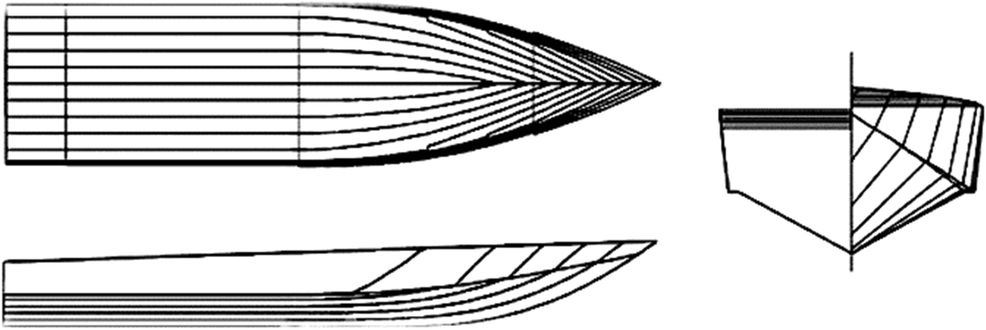Figure  1  Body plans of Cougar planing craft

Download: Full-Size Img

Figure  2  Sample of experimental test for one-step Cougar model conducted in NIMALA

Download: Full-Size Img

2.2   Numerical Procedure

Navier–Stokes and the continuity equations have been used for three-dimensional simulation of flow around the stepped planing craft. The Reynolds averaged version of Navier–Stokes equations has the following Cartesian form:

where Cartesian coordinates are shown by x_i and x_j. In addition, we have velocity components of u_i and u_j, pressure p, density ρ, gravity acceleration g_i, and viscosity μ. In Eq. 2, the Reynolds stress tensor is shown by τ_ij, and it is determinable by an appropriate turbulence model. In addition, μ_eff is an effective viscosity that is μ_eff = μ + μ_t. In the present study, the standard k–ε model is used, which is a confirmed model to simulate the flow around a planing craft (Yousefi et al. 2013).In k–ε model, Reynolds stress has the role of extra eddy viscosity, and this viscosity as a function of fluid flow is as follows:

here, C_μ is a dimensionless constant. In addition, turbulence kinetic energy (Eq. 4) and dissipation rate (Eq. 5) are shown by k and ε, respectively:

where turbulence production by viscous forces is indicted by p_k and C_ε1, C_ε2, σ_ε, and σ_k are constant. Air-water interaction as a free surface is simulated by the volume of fluid (VOF). Transport equation (i.e., to compute the volume ratio between the water and air) in VOF is as follows:

where volume fraction is indicated by α and effective density and viscosity are as follows:

We used VOF with high-resolution interface capturing (HRIC) scheme. In this paper, STAR-CCM+ CFD package (version 10.06) is used that discretized the continuous equations by finite volume method (FVM) via an unsteady solver (CD-Adapco 2015). Semi-implicit method for pressure linked equation (SIMPLE) is implemented to pressure-velocity coupling; second-order SIMPLE approach is applied for convection terms, while diffusion terms are handled by central difference scheme, and time step is calculated for CFL between 0.005 and 0.01 according to ITTC 2014 (ITTC 2014). In addition, we used second-order fully implicit approach for time discretization. In order to have 2DOF dynamics (i.e., free heave and pitch motion), STAR-CCM+ dynamic fluid-body interaction (DFBI) model is used. As may be seen in Figure 3b, computational domain is large enough to prevent from boundary impression on our solutions. Considered boundary conditions are also depicted in Figure 3c. As shown in Figure 3c, inlet velocity according to uniform hull's velocity is used; hydrostatic pressure distribution corresponding to the water depth is applied on flow outlet, and the opening boundary condition is considered, to allow flow existence from top boundary. Moreover, model body surfaces and other boundaries are considered as an impermeable wall with no-slip boundary condition.

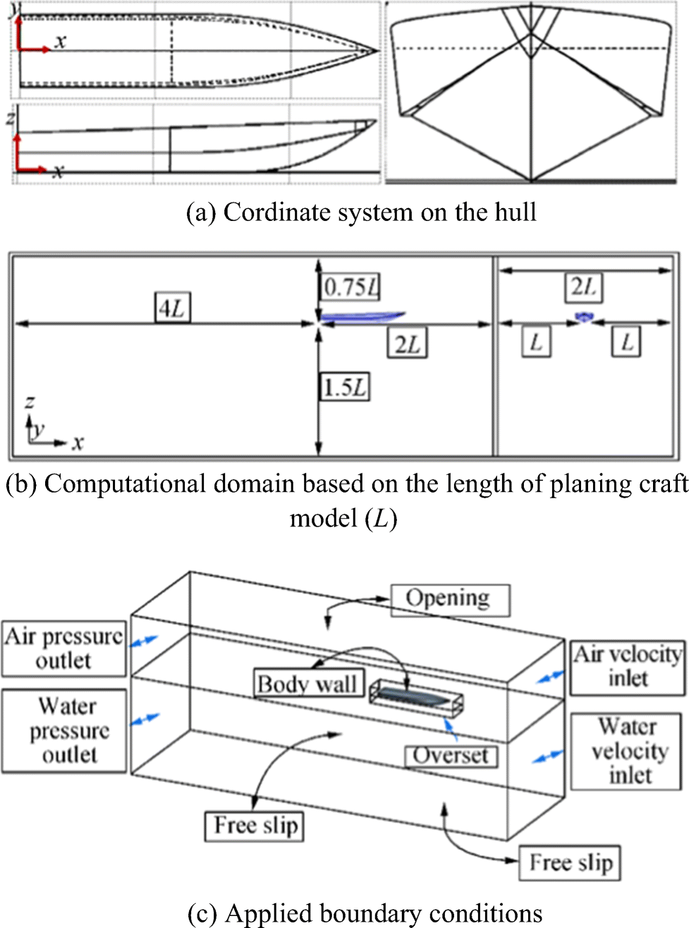Figure  3  Considered boundary conditions

Download: Full-Size Img

2.3   Mesh Sensitivity Analysis

Generated mesh has a significant role in the accuracy of our CFD solution. Hence, in the present paper, dynamic mesh method according to trimmer hexahedral mesh is utilized. In dynamic mesh approach, we used a simple mesh for the entire domain (i.e., background region) with separate meshes (i.e., overset region) for each moving section (Ferziger and Perić 1999). In order to connect the background region with overset region, linear interpolation scheme is used. The accuracy and efficiency of linear interpolation scheme in CFD simulation of planing hulls are shown by De Luca et al. (2016). In addition, some meshes with higher resolution are used at the local positions such as boundary layer, free surface, wake area, and local zones with severe geometrical changes. On the other hand, to investigate the independency of our solution from generated mesh, mesh sensitivity analysis is conducted. As can be seen in Figure 4, in the case of one-step Cougar planing craft, we tested three different meshes, i.e., coarse, medium, and fine grid resolutions at hull velocity 11.502 m/s. The details for values are depicted in Figure 4, and their comparison with experimental data is tabulated in Table 4. Convergence results of grid independency analysis for two-step Cougar planing crafts and their comparison with experimental data are also presented in Table 5. As one can observe in Tables 4 and 5, medium mesh resolution has an insignificant difference compared with fine mesh and, therefore, it is the selected mesh for the current study. It is notable that CFD simulations have been conducted on a computer with an Intel core i7–3.4 GHz processor and 16 GB of RAM. In addition, in case of medium mesh resolution, we compared our CFD results for different hull velocities and loading compared with our experimental data depicted in Tables 6 and 7 and good accordance is obtained. Schematics of the selected dynamic mesh on the Cougar planing craft is depicted in Figure 5. According to the literature review (Jiang et al. 2016), the proper value for $ {y}^{+^{\gamma^{+}}} $ around the planing craft is between 50 and 150. As shown in Figure 6, we achieved an average of y⁺ about 80 for one-step Cougar planing craft.

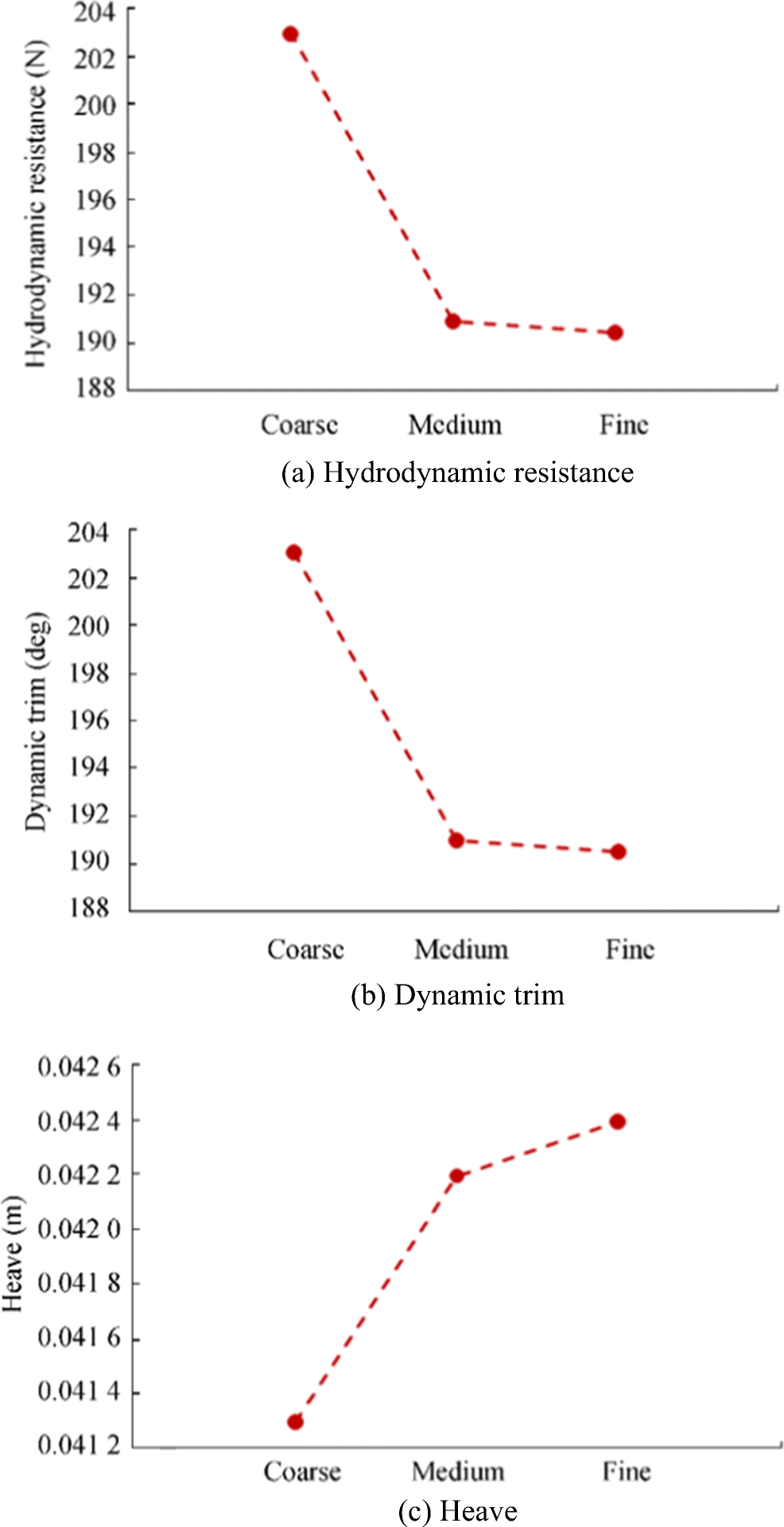Figure  4  Numerical convergence results in grid independency analysis for one-step Cougar planing craft

Download: Full-Size Img

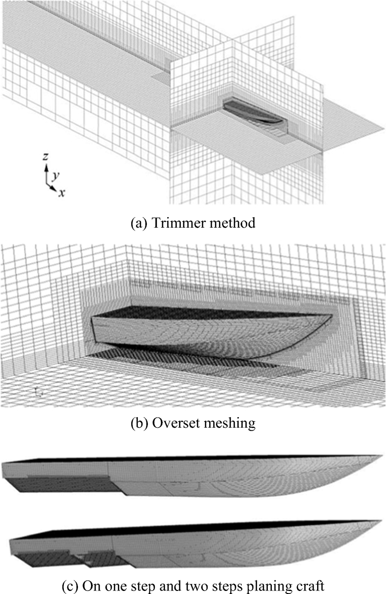Figure  5  Schematic of dynamic meshes on Cougar planing craft

Download: Full-Size Img

Figure  6  Parameter of y⁺ on the bottom surface of Cougar planing craft under dynamic mesh method

Download: Full-Size Img

Now, based on grid convergence method (CGI) that is suggested by Celik et al. (2008), we performed a formal verification for our mesh sensitivity analysis. In CGI, an average of apparent order of method has the following form:

here,

where the correction factor for three different mesh in the present study is $ {r}_{21}=\sqrt{2} $ and $ {r}_{32}=\sqrt{2} $. In addition, in this method, for considered calculated parameter of φ, we have ε₂₁ = φ₂ − φ₁ and ε₃₂ = φ₃ − φ₂. Now, extrapolated value (Eq. 10), defined approximated relative error (Eq. 9), extrapolated relative error (Eq. 12), and fine-grid convergence index (Eq. 13) are as follows:

In Table 8, these parameters are calculated for considered hydrodynamics resistance, dynamic trim, and heave. As may be seen in Table 8, maximum uncertainties are obtained: $ {\mathrm{GCI}}_{\mathrm{fine}}^{32}=7.81\% $ for hydrodynamics resistance, $ {\mathrm{GCI}}_{\mathrm{fine}}^{32}=6.99\% $ for dynamic trim, and $ {\mathrm{GCI}}_{\mathrm{fine}}^{32}=7.79\% $ for heave.

Continued, fundamental of ANN method to predict hydrodynamic resistance of considered stepped planing craft under different considered conditions, is presented.

3   Artificial Neural Network Structures

Artificial neural networks (ANN) as an interesting soft computing method is able to predict the complicated physical system by generating learned interconnection between the different input parameters to the considered output via process units (i.e., neurons) in different hidden layers. So, in each ANN structure, three layers of input layer, hidden layer, and output layer are evident. Different learning methods are suggested to train the ANN, and feed-forward back-propagation is one of the interesting deep learning methods that are used in the present paper. Neurons of input layer are the host of outside evidence, and this evidence will be transmitted to the input variable by an identity transfer function. Afterward, weighted data transfers through the interconnection between the input neurons and hidden layer neurons. Then, the processed data in the hidden layer added via bias and transfer function will be applied to their summation. We used hyperbolic tangent sigmoid transfer function in the hidden layer as follows:

here, jth neuron of output is shown by n_j, ω_ij is the interconnection weight from ith neuron in the previous layer to the jth neurons, and p_i is the output. In addition, r is the number of previous layer neurons, while bias is indicated by b_j. Then, as stated before, by linear transfer function λ applied on the summation of hidden layer neurons, the output intended parameter is identified:

here, the interconnection weights ω_L are between the last hidden layer and output layer and output layer bias is shown by b_o. As stated before, we used feed-forward neural networks with back-propagation (BP) learning procedure that is suggested by Rumelhart et al. (1986). To optimize the ANN, Marquardt–Levenberg algorithm (MLA) is utilized. In back-propagation method, the learning algorithm is based on the propagation of backward errors via a stochastic gradient descend approach. In addition, MLA is used as offline training in the role of the damped least-squares (DLS) scheme.

In order to assess the performance efficiency of ANN, we have used mean square errors (MSE) and correlation coefficient (R) as follows (Armstrong and Collopy 1992; Wheelwright et al. 1998):

As may be seen in Eqs. 16 and 17, N is the number of evidence data, y_desired is representative of the desired data, O_i is the predicted results or actual values, and the average of desired values is shown by $ {\overline{y}}_{\mathrm{desired}} $. In the present paper, we provided a database of ANNs by 135CFD data that the ranges of intended input–output variables are presented in Table 9.

We randomly classified our CFD data into train data (60% of inputs–outputs to adjust the ANN's weights), validation data (20% of inputs–outputs for minimizing the overfitting and tuning the ANN's weights), and test data sets (20% of inputs–outputs for testing the final solution of ANN). Early stopping approach (Prechelt 1999) is also used to prevent over-fitting. In this study, relative to various magnitudes of our data, all the input–output data are normalized between 0.1 and 0.9 as follows:

Now, the number of hidden layer and neurons is significant for selecting an appropriate ANN structure to predict hydrodynamic resistance based on the considered inputs. According to literature and our experience, one and two hidden layers are more interested due to their logical computational cost and their well performance (Choi et al. 2008; Trenn 2008). Therefore, we used two hidden layer architectures for the intended ANN. To select an appropriate number of neurons in each layer, we used an iterative algorithm that is illustrated in Figure 7. Basic concepts of our algorithm are expressed in Refs. (Shora et al. 2018; Nowruzi et al. 2017b). We performed the procedure of the proposed algorithm in Figure 7, and an appropriate ANN with two hidden layers and architecture of 5:7:5:1 is achieved (see Figure 8).

Figure  7  Iterative algorithm to select an appropriate architecture for ANN

Download: Full-Size Img

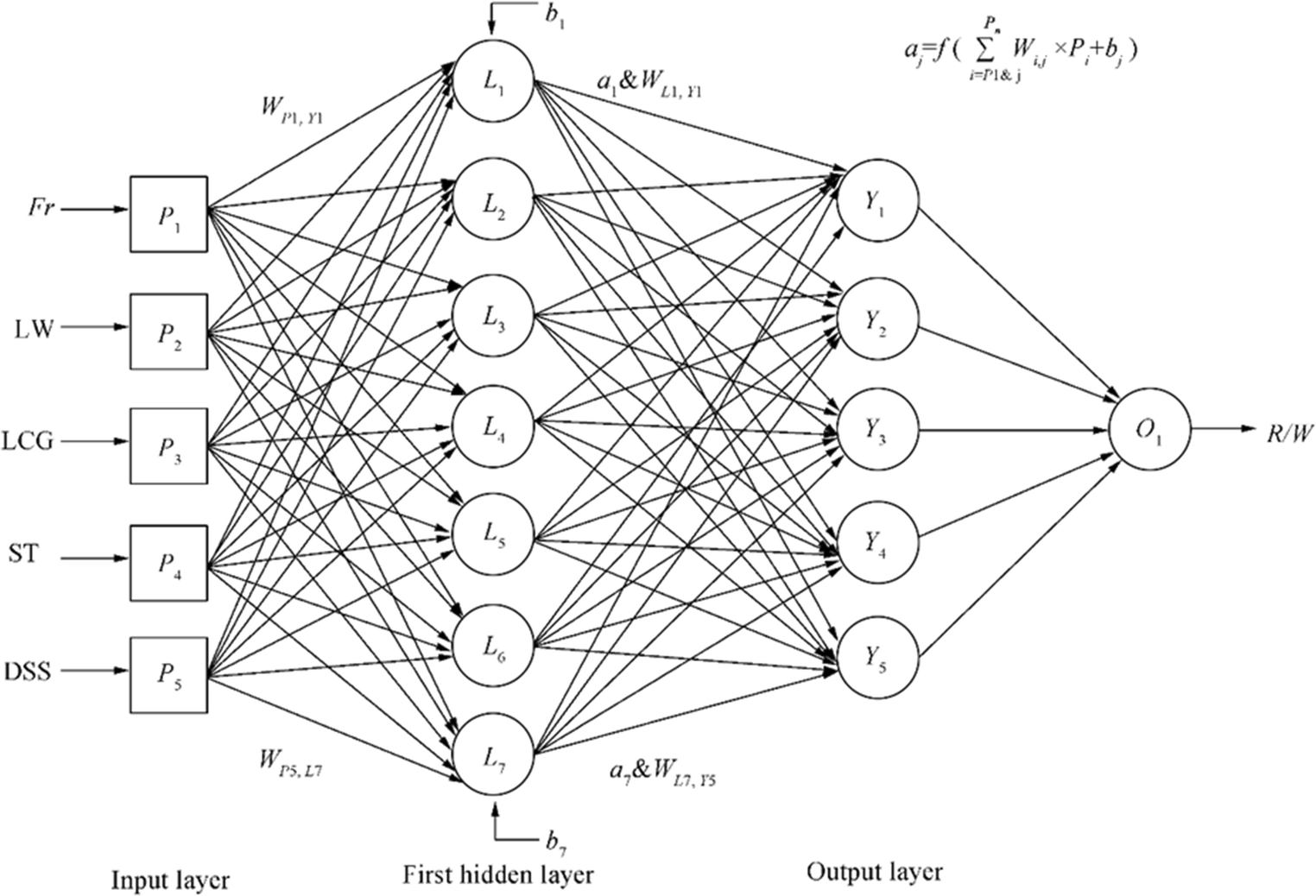Figure  8  Architecture of selected ANN for prediction of hydrodynamic resistance to weight ratio of intended stepped planing crafts

Download: Full-Size Img

4   Results and Discussion

In the current section, preliminarily, the CFD results of hydrodynamic resistance to weight ratio and some of the pressure distribution, wave pattern, and streamlines around the hull models are presented and discussed. Afterward, correlation diagrams, predictive equation, and weight sensitivity analysis based on selected ANN are presented.

4.1   CFD Results

To investigate the hydrodynamic resistance to weight ratio of considered planing craft in different hull types of without step, one step, and two steps (with different DSS), R/W vs Froude number under different LCG positions from aft are presented for weight loads of 76 kg, 84 kg, and 92 kg, in Figures 9, 10, and 11, respectively. As may be seen in Figures 9, 10, and 11, at lower weight load conditions and for larger DSS, using steps will result in greater resistance to weight ratio (R/W). Indeed, in these conditions, planing crafts without any steps give lower R/W compared with stepped planing crafts; the reason for this might be related to the increase of frictional resistance and stream-wise separation on the steps. However, as the weight loading increases and DSS decreases, the R/W for stepped planing craft decreases compared with the case of without step crafts. In addition to this, as depicted in Figure 9a, in the case of LCG 27%L, porpoising has occurred for without step; thus, we cannot report any value for R/W for without step planing crafts at Fr > 5, while, using step may cause a delay in porpoising. This might be because of proper air ventilation, formation of stream-wise separation, and lower interaction between first and second steps for greater weight loading and smaller DSS. Furthermore, as shown in Figure 9a, R/W for DSS 17%L is approximately similar to the R/W of one-step planing craft. According to Figure 10, at LCG 27%L, porpoising has occurred for one step at Fr > 5 and in the case of without step at any Fr. The trend of R/W enhancement by an increase of Fr, larger LCG%L and DSS for the 84 kg weight loading is similar to the 76-kg weight loading (Figure 9). Figure 11 also indicates that in some critical cases, due to lack of proper air ventilation and larger LCG%L, greater R/W is obtained for stepped planing craft compared with the case of without step. More details related to dynamic trim angle, dynamic sinkage, and total wetted area for without step, one-step, and two-step (with different DSS) planing crafts at weight loading 76 kg under different LCGs and Froude numbers are also presented in Appendix 1.

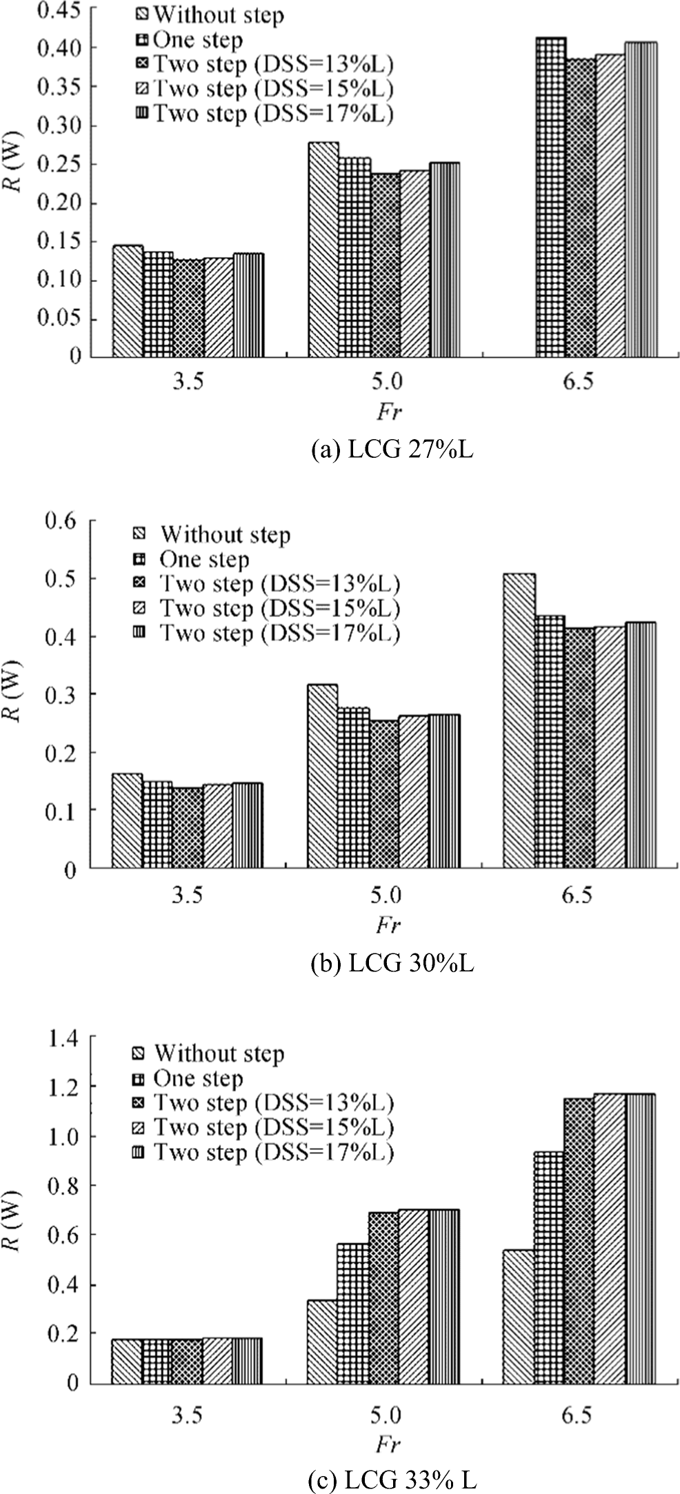Figure  9  Hydrodynamic resistance to weight ratio for without step, one step and two steps (with different DSS) planing craft at weight loading 76 kg

Download: Full-Size Img

Figure  10  Hydrodynamic resistance to weight ratio for without step, one step and two steps (with different DSS) planing craft at weight loading 84 kg

Download: Full-Size Img

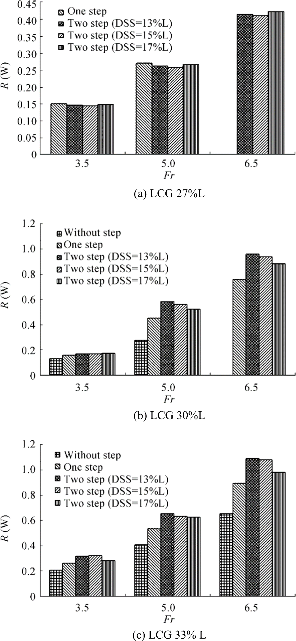Figure  11  Hydrodynamic resistance to weight ratio for without step, one step and two steps (with different DSS) planing craft at weight loading 92 kg

Download: Full-Size Img

To better study the hydrodynamics performance of considered stepped planing craft, bottom pressure distribution at three different hull forms (i.e., without step, one step, and two steps) under three different Froude numbers are presented in Figure 12. As may be seen in Figure 12, wetted area is slightly enhanced by an increase in the Froude number that may be related to the very low reduction of dynamic trim angle at upper hull velocities. In addition, N + 1 local high-pressure region is visible, where N is the number of steps and these regions are corresponding to stagnation point of separated flow on the steps. So, the local region with a minimum of pressure is also detectable exactly before these local high-pressure regions. Moreover, as the Fr increases, the effective area of these high-pressure regions is increased and moved into the fore-body that may increase the possibility of porpoising. Lower wetted area is depicted by using steps compared with the case without step. Also, positive impression of two steps compared with one step on the reduction of wetted area is evident. Moreover, we can see wetted surface region on the chine which are related to fluid flow separation and spray from chine. This phenomenon is also reported by Bakhtiari et al. (2016). Finally, more uniform pressure distribution is also achieved by using two-step planing craft compared with one-step hull.

Figure  12  Bottom pressure distribution in case of without step, one-step, and two-step planing craft under three different Fr (at weight loading 76 kg and LCG 33%L)

Download: Full-Size Img

Figure 13 shows the distribution of bottom frictional drag coefficient at three different hull forms (i.e., without step, one step, and two steps) under three different Fr. Based on Figure 13, the area of local region with maximum frictional drag coefficient is reduced by the increase of the Fr. Moreover, as the hull is equipped by steps, the value and effective area of frictional drag coefficient are decreased. This advantage of stepped planing crafts compared with without step hull is one of the main reasons for selection of stepped planing craft.

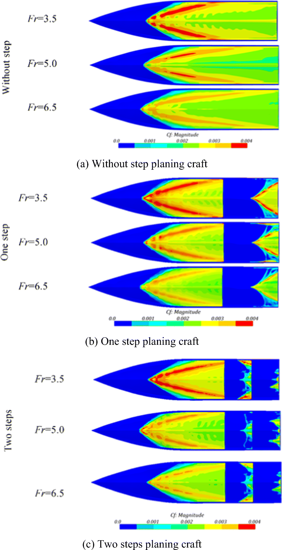Figure  13  Bottom frictional drag coefficient in case of without step, one-step, and two-step planing craft under three different Fr (at weight loading 76 kg and LCG 33%L)

Download: Full-Size Img

4.2   ANN Results

As stated in Section 3, to predict the resistance to weight ratio of considered stepped planing craft under different Froude number (Fr), loading weight (LW), LCG position from aft as %L (LCG), step type (ST), and distance of second step from aft as %L (DSS), ANN via the architecture of 5:7:5:1 is selected. Figure 14 shows the correlation diagrams for used data and predicted values of R/W for training, validation, test, and all data. As may be observed in Figure 14, an appropriate correlation is achieved for reference CFD data and predicted output of ANN. Moreover, we obtained the maximum MSE and lowest correlation coefficient, which are equal to 0.0027 and 0.97091, respectively. In Figure 15, we compared the results of used data and predicted outputs of ANN for training, validation, test, and all data sets. Based on Figure 15, the predicted output shows acceptable accordance compared with used data.

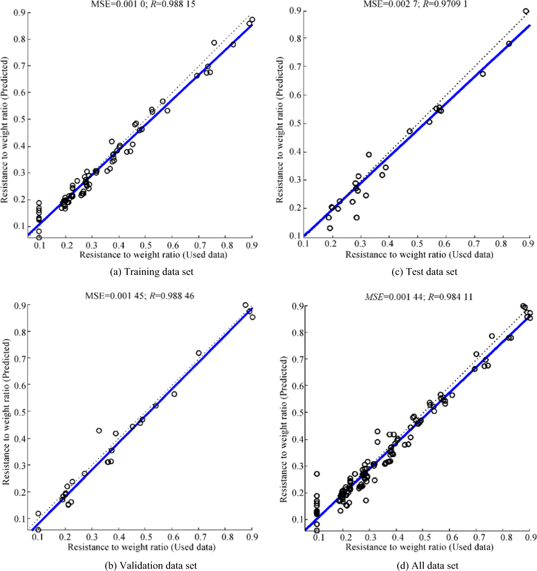Figure  14  Correlation between the used data values and predicted outputs for resistance to weight ratio

Download: Full-Size Img

Figure  15  Comparison between the used data results and predicted outputs of resistance to weight ratio

Download: Full-Size Img

Based on Figures 14 and 15, the designed ANN is capable of predicting resistance to weight ratio of stepped planing craft under different Fr, LW, LCG, ST, and DSS, appropriately. Thus, according to the weights and bias of selected ANN, we proposed an equation to predict the resistance to weight ratio under different considered geometrical and physical conditions. The proposed equation is as follows:

where H has the following form:

where, y_j is in the following form:

Constant values of Eqs. 20 and 21 are presented in the Appendix 2. To verify the proposed equation, some experimental data of R/W for different types of without step, one-step, and two-step Cougar planing crafts are compared with the predicted results of proposed equation in Table 10. As may be seen in Table 10, the proposed equation predicted the R/W with an appropriated accuracy (error less than 6.6% compared with experimental data).

Another interesting analysis of the output of ANN is weight sensitivity analysis. This analysis shows the relative effect percentage of each input variable on the ANN output by manipulation of weight matrixes. Garson (1991) presented the partitioning of the ANN weights method, as follows:

where the output of Eq. 22 shows the relative importance of each input on the considered output of ANN. In addition, the numbers of hidden layer inputs and neurons are indicted by N_i and N_h associated with weight of ω. Input, hidden, and output layers are characterized by indices of "i, " "h, " and "o", respectively. Input, hidden, and output neurons are also respectively characterized by indices of "k, " "m, " and "n." Figure 16 shows relative importance of the input variables Fr, ST, LCG, WL, and DSS on the response variable of resistance to weight ratio of considered stepped planing craft. As may be seen in Figure 16, the largest effect is achieved for LCG with relative importance percentage of 27.44%, while WL with relative importance percentage of 14.29% has the lowest impression on the resistance to weight ratio.

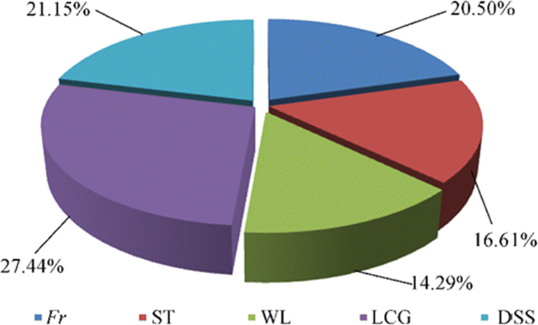Figure  16  Relative importance of the input variables Fr, ST, LCG, WL and DSS on the response variable of resistance to weight ratio of considered stepped planing craft

Download: Full-Size Img

5   Conclusion

Stepped planing crafts are considered as favorite high-speed vessels. One of the most important factors, in order to improve their design, is the prediction of the hydrodynamic resistance of these crafts. Hydrodynamic resistance of stepped planing craft is significantly related to the Froude number, weight loading, number of steps, shape of the step, step height, position of first and second steps, and LCG. In the current study, hydrodynamic performance of without step, one-step, and two-step Cougar planing craft, stepped planing craft under different Froude number, different distances of second step and LCG from aft body, and various weight loads are numerically studied. To this accomplishment, the accuracy of our CFD results after mesh sensitivity analysis is properly validated against our conducted experimental tests. Then, by designing proper ANN, resistance to weight ratio is predicted under considered geometrical and physical conditions. The most significant results of the presented research are as follows:

1)  The value of resistance to weight ratio is decreased by using steps at higher weights and lower LCG distance from aft body, where reduction of distance between two steps (DSS) causes greater resistance value.

2)  The undesirable phenomenon of porpoising is delayed by using steps on the bottom of planing craft and increasing the number of steps form one-step to two-step results in more longitudinally stable crafts.

3)  The maximum value of MSE in the prediction of hydrodynamic resistance to weight ratio by selected ANN is obtained 0.0027. The minimum correlation coefficient (R) value is also calculated 0.97091.

4)  Based on the ANN weight sensitivity analysis, LCG with relative importance percentage of 27.44% is a more efficient factor on resistance to weight ratio of considered stepped planing craft, while WL with relative importance percentage of 14.29% has the lowest impression.

5)  A predictive equation according to designed ANN weights and bias is suggested to predict resistance to weight ratio of stepped planing crafts under different Froude numbers, weight loads, number of steps, position of second steps, and LCGs.

The proposed methodology in current study may be utilized as a reference to estimate the resistance to weight ratio of different type of stepped planing crafts under various positions of steps, LCGs, weight loadings, and Fr numbers.

Appendix 1

In this appendix, dynamic trim angle, dynamic sinkage, and total wetted area for without step, one-step, and two-step (with different DSS) planing crafts at weight loading 76 kg under different LCGs and Froude numbers are tabulated in Table 11.

Appendix 2

Constant values of Eqs. 20 and 21 are presented in Table 12.