1   Introduction

Ships, in general, may experience three types of displacement motions (heave, sway or drift, and surge) and three angular motions (yaw, pitch, and roll) as depicted in Figure 1. Ship roll reduction or stabilization consists of two main parts: The first is the roll reduction or stabilization method, and the second is the evaluation or modeling method of the roll performance. Started with Froude (1861), roll motion and related topics have been studied since the late-mid 1800s. For example, Tanaka (1961), Kato (1965), and Ikeda et al. (2004) studied roll damping based on theory, numerical calculation, and experimentation and suggested an empirical formula including the effect of a bilge keel. A simple method for predicting the roll damping of a ship at forward speed was proposed by Himeno (1981) while Ikeda suggested a modified model (Ikeda et al. 2004).

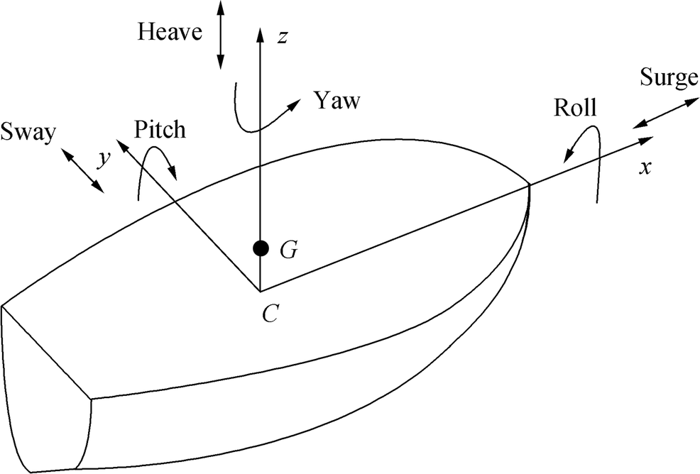Figure  1  Schematic diagram of ship showing the six degrees of freedom

Download: Full-Size Img

The dynamic roll characteristic has been one of the most central topics in sea keeping study. However, due to the complexity induced by high nonlinearity, potential flow methods cannot solve the roll motion problems effectively. Up to date, many research groups have adopted various methodologies, including the advanced experimental process, empirical formulas, or computational fluid dynamics (CFD). One of the topics is related to the characteristics of roll motion for bare hull and with different appendages. Another branch of related research has focused on the analysis method for roll damping, which includes a higher polynomial roll damping model, finite differential model, or hyperbola model. Recently, CFD-based methods have been used for the analysis of local phenomena such as vortex shedding around bilge keels (Yeung et al. 1997).

Several authors have studied roll damping experimentally for local flow visualization (see, for example, Aloisio and Felice 2006; Bassler et al. 2007; Oliveira and Fernandes 2012). On the other hand, mathematical modeling of roll damping has been investigated by researchers, for example, Oliveira and Fernandes (2014) used the bilinear or hyperbola fitting method, and Agarwal (2015) used a fractional differential equation model. However, modeling damping motion in terms of a second-order ordinary differential equation (quadratic model) is widely accepted. Recently, Oliveira and Fernandes (2012) discussed the nonlinear roll damping of FPSO hull. Although these methods have advantages, especially for newer hull designs or nontypical appendages in terms of shape and size, the traditional methods for a typical design have not yet been fully validated.

Behavior analysis of a ship affected by external forces and analysis of ship stability in waves are based on more complex mathematical models as a result of strong nonlinear terms in the governing equations of these systems. Nonlinear analysis makes it possible to comprehend the theory of ship behavior for forecasting stability changes in various conditions of operation. In addition, ship turning motion is an important part of ship maneuverability and is directly related to the safety of a sailing (Lihua et al. 2018). The flow in the vicinity of 2D ship sections carrying out forced roll motions is simulated using the solution of the Navier-Stokes equations (Lavrov et al. 2017). A new coarse and fine-tuning fixed grid wavelet network is proposed for online predicting ship roll motion in regular waves (Huang et al. 2018). Kianejad et al. (2019) improved prediction of a ship roll motion in parametric roll and dead ship using CFD. Another important related topic that has been under investigation is fin stabilizer control. Demirel and Alarcin (2016) used LM-based H₂ and H_∞ state-feedback controller for fin stabilizer of a fishing boat and also presented a backstepping control design procedure for nonlinear fin roll control of a trawler (Demirel et al. 2017).

The second-order nonlinear differential equation modeling the ship roll motion does not have a closed-form solution. Despite the fact that reliable numerical and experimental methods have been implemented to find approximate solutions, the need for analytical solutions is still a necessity in order to understand the effect of parameters' variation on the governing system. Of the well-established methods that can be employed to obtain analytical expressions of roll angle, velocity, and damping and restoring moments, we mention the variational iteration method (Lu 2007; Abukhaled 2013), differential transformation method (Chen and Liu 1998), Green function based method (Khuri and Abukhaled 2017; Abukhaled 2017), finite element method (Comini et al. 1970), series method (Salomi et al. 2020), homotopy perturbation method (He 1999), and homotopy analysis method (Liao and Chwang 1998; Liao 1997; Liao 2004). Another approach that can be employed is that the differential equation may be analyzed based on the formulation of an equivalent integral equation (Jang et al. 2009; Jang 2011; Jang 2013).

In this project, the governing equation will be solved analytically by using a modified form of the homotopy perturbation method and numerically by using a high-order ultraspherical wavelets–based method. Wavelet-based methods using operational matrix of derivatives are accurate and reliable and have been intensively used in many fields of science and engineering applications. For example, wavelet-based methods are used to find approximate solutions for nonlinear differential equations (Salai Mathi Selvi et al. 2017), for Michaelis-Menten enzymatic reaction equation Salai Mathi Selvi and Hariharan (2017), and for solving integro-differential equations (Tavassoli Kajani and Hadi Vencheh 2004). Wavelet-based methods have also been employed to solve optimal control and fractional optimal control problems (Razzaghi and Yousef 2002; Sadek et al. 2007; Abualrub et al. 2018). Recently, Salai Mathi Selvi and Hariharan (2016) applied the Chebyshev wavelet algorithm for solving steady-state concentration of packed-bed reactor model, Zheng and Wei (2016), used Legendre wavelets to estimates the error of approximation when solving integral equations, and Abualrub and Abukhaled (2015) employed wavelets to regulate cellular processes for the growth or regeneration of a tissue within an assigned terminal time.

This paper is organized as follows: Section 2 describes the mathematical formulation of the problem. Section 3 discusses the properties of ultraspherical wavelets and a wavelet-based solution method. In Section 4, the homotopy perturbation method for obtaining an analytical solution is explained. Illustrative examples are presented in Section 5 with their discussions in Section 6. Finally, Section 7 presents our conclusions.

2   Mathematical Formulation of the Problem

Under the assumption of independent oscillation, the nonlinear rolling motion of a ship is described by the differential equation (Cardo et al. 1981)

where ϕ is the roll angle to the calm sea surface and $ \dot{\phi} $ and $ \ddot{\phi} $ are the roll velocity and acceleration, respectively. Equation (1) represents the general equation of roll motion of ships in the absolute heeling angle, where the motion is induced by regular transversal waves. I is the mass moment of inertia including added mass moment (kg · m²), $ D\left(\phi, \dot{\phi}\right) $ is the moment of the dissipative forces (N · m), M_r(φ, t) is the righting moment (N · m), and E_w represents the amplitude and Ωis the angular frequency. In this study, the nonlinear damping term is assumed to take into consideration an angular dependence of the linear term, that is,

and the righting moment is expressed in the normalized form

Introducing the angle and time scales ϕ_n and T_n, the following dimensionless parameters can be defined

then, using these parameters and rearranging terms gives the following cubic damping moment of nonlinear roll motion (Cardo et al. 1981)

where $ {\omega}_0^2 $ is the dimensionless angular frequency, ω is the frequency, α is strength of nonlinearity coefficient, μ is dimensionless damping coefficient, δ₁ and δ₂ are quadratic viscous damping coefficients, and ε is the amplitude.

3   Properties of Ultraspherical Polynomials and Their Shifted Forms

In this section, we use the function presentation via shifted ultraspherical wavelets to construct a wavelet-based method to obtain a numerical solution for the governing Eq. (5). Appendices 1 and 2 provide simple prelude to this section (see Doha et al. 2016 and the references therein for more in-depth details).

3.1   Shifted Ultraspherical Wavelets and Function Representation

Ultraspherical wavelets $ {\psi}_{nm}^{\left(\alpha \right)}\left(\xi \right)=\left(k,n,m,\alpha, \xi \right) $ are defined on the interval [0, 1] by Doha et al. (2016).

where m = 0, 1, 2, …M, n = 0, 1, 2, …2^k − 1, m is the constructed polynomial order, α is a prescribed parameter, ξ the normalized time, and

A function f(t) defined on [0, 1] may be expanded in terms of ultraspherical wavelets as

where

Using the truncated finite series, f(t) can be approximated in terms of ultraspherical wavelets as

where

3.2   Operational Matrix of Derivatives

The operational matrix of derivatives is given by the following theorem.

Theorem 1 For the ultraspherical wavelets vector (12),

where D is a 2^k(M + 1) × 2^k(M + 1) operational matrix given by

in which F is an M + 1 square matrix whose (r, s)th entry is given by

Proof See Doha et al. (2016).

The following theorem states that the ultraspherical wavelet expansion of a function f(t), with a bounded second derivative, converges uniformly tof(t).

Theorem 2 A function $ f(t)\in {L}_{\overset{\sim }{\omega}}^2\left[0,1\right],\overset{\sim }{\omega }={\left(t-{t}^2\right)}^{\alpha -\frac{1}{2}},0 \lt \alpha \lt 1 $ can be expanded as an infinite series of ultraspherical wavelets, which converges uniformly to f(t), provided that f " (t) ≤ L.

Moreover,

Proof See Doha et al. (2016).

3.3   Wavelet-Based Numerical Solution

The wavelet-based method for finding a numerical solution for a homogenous or nonhomogenous nonlinear equation describing the roll motion of a ship begins by using ultraspherical wavelets expansion along with a spectral collocation method to reduce the governing initial value problem into a system of algebraic equations with unknown coefficients.

For finding an approximate numerical solution for Eq. (5), we begin by expanding x(t) and the function g(t) = cos ωt in terms of ultraspherical wavelets as follows

Using the operational matrix of derivatives gives

Now substituting Eqs. (17)–(19) into Eq. (5) gives the residual written explicitly as

4   Analytical Solution Using a New Approach of HPM

A brief introduction to the basic concept of the homotopy perturbation method is delineated in Appendix 3.

As per Eq. (4) (Appendix 3), the homotopy of Eq. (5) takes the form.

where p ∈ [0, 1] is an embedding parameter. The approximate solution of Eq. (35), expressed in a power series, is

By letting p = 1, an analytical solution, in the form of series expansion, is derived.

5   Illustrative Examples

In this section, we apply the analytical HPM method and the numerical ultraspherical wavelet method to cubic damping moment of nonlinear roll motion.

Example 1 Consider the nonlinear BVP (Cardo et al. 1984)

where the experimental values of the parameters are $ \mu =0.005,{\delta}_1=0.1,{\omega}_0^2=1,\mathrm{and}\ {\alpha}_3=-1.75. $

Using the ultraspherical wavelet method, we substitute Eq. (17) and Eq. (19) into Eq. (23) to obtain

Also using Eq. (17) and Eq. (19), the initial conditions given in Eq. (38) become

where the operational matrix of derivatives is

in which

Now, the approximate wavelet solution x(t) is

where the vector ψ^(α)(t) is given by

and the constants vector C is given by

To find the HPM analytical solution for Eq. (23), we use the homotopy in Eq. (21) to find that the coefficient associated with p⁰ is the nonlinear equation

Now x₀ is obtained by solving Eq. (32) subject to initial conditions

In a similar fashion, the nonlinear differential equation associated with p¹ can be obtained and then solved for x₁.

Using only two terms of Eq. (22) with p = 1, we obtain the following approximate analytical solution of Eq. (23)

Example 2 Consider the cubic damping moment of nonlinear roll motion represented by the IVP (Cardo et al. 1984)

We will consider three sets of experimental values for the parameters.

Case 1 Assume that

Using the ultraspherical wavelet method, we substitute Eqs. (17) and (19) into Eqs. (42) and (43) to obtain

and

As detailed in the example above, the approximate numerical wavelet solution, x(t), is expressed in the form

Applying the proposed approach of the HPM to Eq. (35) gives the following analytical expression for the roll angle at any time t:

The velocity and acceleration are, respectively, given by

Rearranging terms gives the cubic restoring moment formula

and the cubic damping moment formula

Case 2 Assume the following experimental values of the parameters: $ \mu =0.02,{\delta}_1=0.1,{\omega}_0^2=1,{\alpha}_3=-1.75,\varepsilon =0.2,\mathrm{and}\ \omega =0.33333. $

The numerical wavelet solution is given by Eq. (39) where Ψ^(α)(t) is obtained by solving the equation

subject to the initial conditions given in Eq. (38). The HPM analytical solution is

Case 3 Assume the following experimental values of the parameters: $ \mu =0.02,{\delta}_1=0.1,{\omega}_0^2=1,{\alpha}_3=4,\varepsilon =0.2,\mathrm{and}\ \omega =0.33333. $

The numerical wavelet solution is given by Eq. (39) where Ψ^(α)(t) is obtained by solving the equation

subject to the initial conditions given in Eq. (38).

The analytical solution obtained by the HPM is given by

Example 3 Consider the cubic damping moment of nonlinear roll motion represented by the IVP (Liao and Chwang 1998)

where the experimental values of the parameters are η = 0.1, b = 0.5, and l = 0.2.

Using the ultraspherical wavelet method, we obtain the approximate solution

where Ψ^(α)(t) is obtained from the equation

subject to the initial conditions take the from

In order to apply the homotopy perturbation method, we first construct the following homotopy equation

The solution and the coefficient of the linear term are expanded in the forms in Eqs. (3) and (4)

By substituting Eqs. (55) and (56) into Eq. (54), the following linear differential equation system is obtained

Solving Eq. (57) for x₀ gives

Substituting Eq. (59) into Eq. (58) leads to

or

No secular term in x₁ requires that

or

The first-order approximate from Eq. (55) is

and hence from Eqs. (63) and (64), the following frequency is readily obtained

Also, from Eq. (59), we obtain the velocity expression

6   Results and Discussion

The proposed methods are applied to investigate a steady-state roll motion of a ship with nonlinear damping and restoring moments. A comparison between the numerical results obtained by the ultraspherical wavelet method (UWM), the analytical results obtained by a new approach of the homotopy perturbation method (HPM), and numerical simulations obtained by the fourth-order Runge-Kutta method (numerical) is discussed.

Roll angle decay curves in Example 1 are obtained by UWM (Eq. (29)) and the HPM (Eq. (34)). Figure 2 shows that these methods are in excellent agreement with the numerical solution obtained by RK4. Figure 3 also shows an excellent agreement between the UWM solution (Eq. (39)), the analytical solution (Eq. (40)), and RK4 for the roll angle decay of Example 2, Case 1. The curves in Figures 2 and 3 resemble the large amplitudes roll angles due to cubic damping moments and show that the motion continues indefinitely when only conservative forces act, and thus, the mechanical energy remains constant. Figure 4 shows that the velocity curves in Example 2 Case 1obtained by the modified HPM (Eq. (41)) and RK4 are identical. In Figures 5, 6, and 7, the curves of acceleration (Eq. (42)), restoring moment (Eq. (43)), and damping moment (Eq. (44)) are plotted, respectively, against time using the analytical HPM. Roll angle decay curves for Example 2, Cases 2 and 3, are shown, respectively, in Figures 8 and 9, while Figure 10 represents the roll angle decay curves for Example 3 using the proposed methods. Figure 11 depicts the displacement and velocity with weak nonlinearity and small amplitude. The envelopes of nonlinear ship roll motion, velocity, and acceleration are depicted in Figures 12 and 13. The frequency curves versus roll motion, velocity, and acceleration are given in Figures 14, 15, and 16.

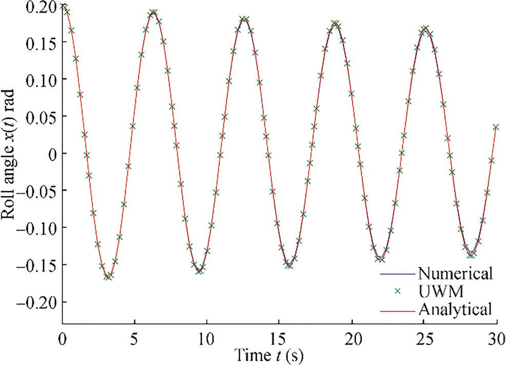Figure  2  Comparison of UWM, HPM, and NM for roll angle decay curve in Example 1

Download: Full-Size Img

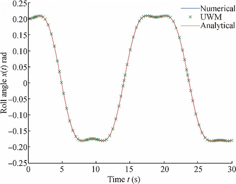Figure  3  Comparison of UWM, HPM, and NM for roll angle decay curve in Example 2, Case 1

Download: Full-Size Img

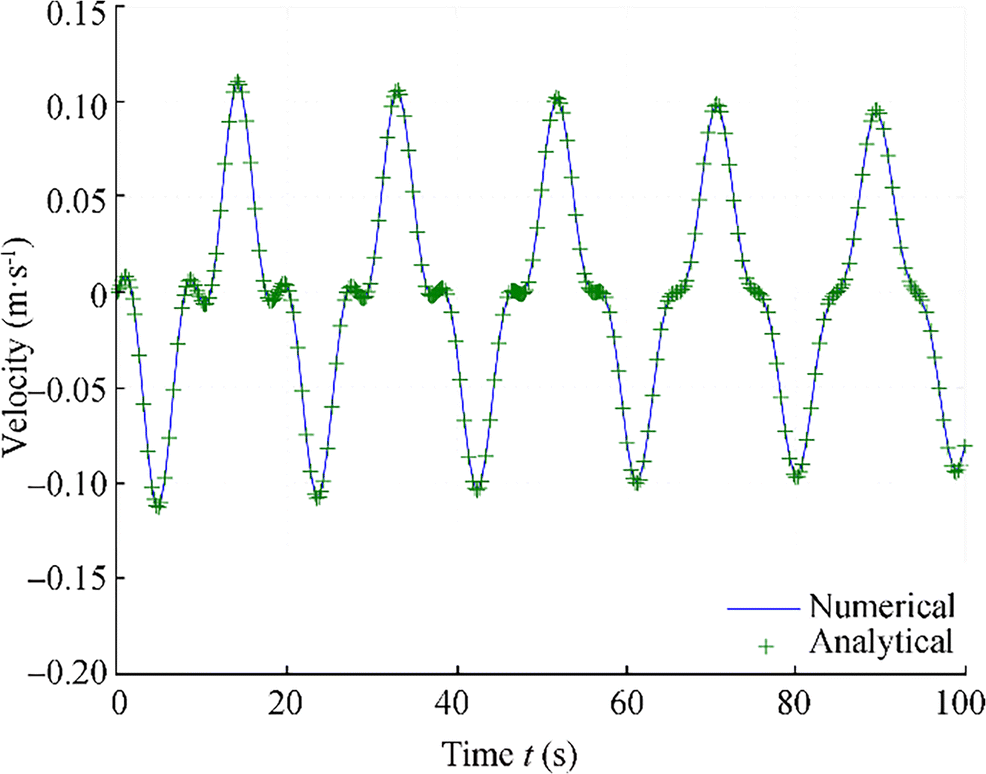Figure  4  Comparison between the HPM and NM for the velocity curve in Example 2, Case 1

Download: Full-Size Img

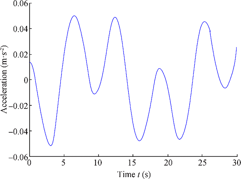Figure  5  Plot of analytical expression of the acceleration curve in Example 2 Case 1

Download: Full-Size Img

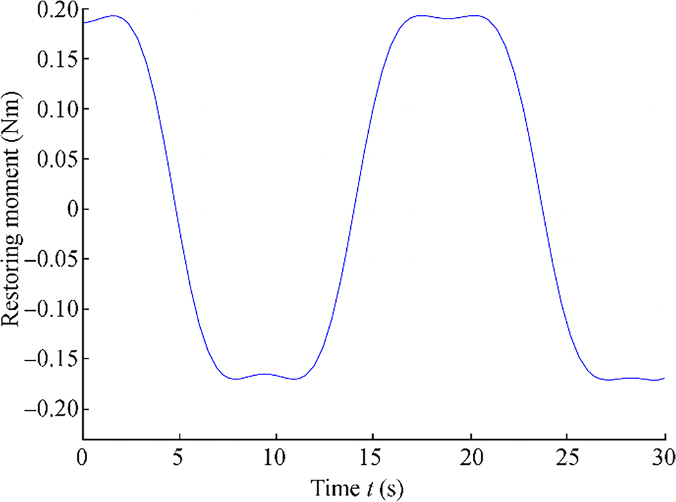Figure  6  Plot of restoring moment versus time, Eq. (43)

Download: Full-Size Img

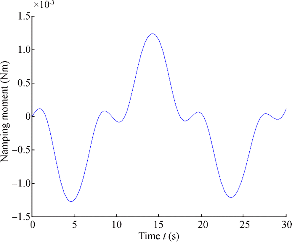Figure  7  Plot of damping moment versus time, Eq. (44)

Download: Full-Size Img

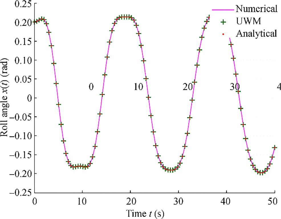Figure  8  Comparison of UWM, HPM, and NM for roll angle decay curve in Example 2, Case 2

Download: Full-Size Img

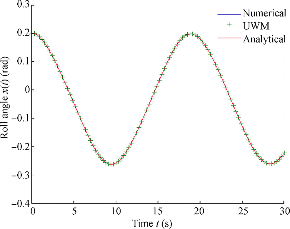Figure  9  Comparison of UWM, HPM, and NM for roll angle decay curve in Example 2, Case 3

Download: Full-Size Img

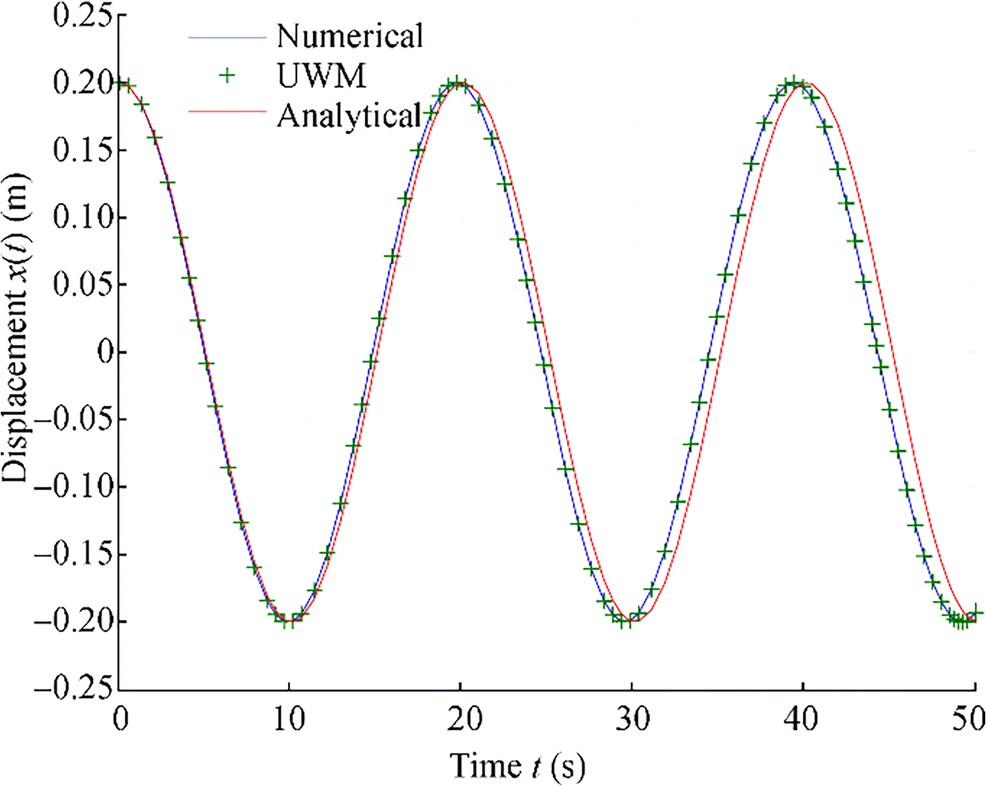Figure  10  Comparison of UWM, HPM, and NM for roll angle decay curve in Example 3

Download: Full-Size Img

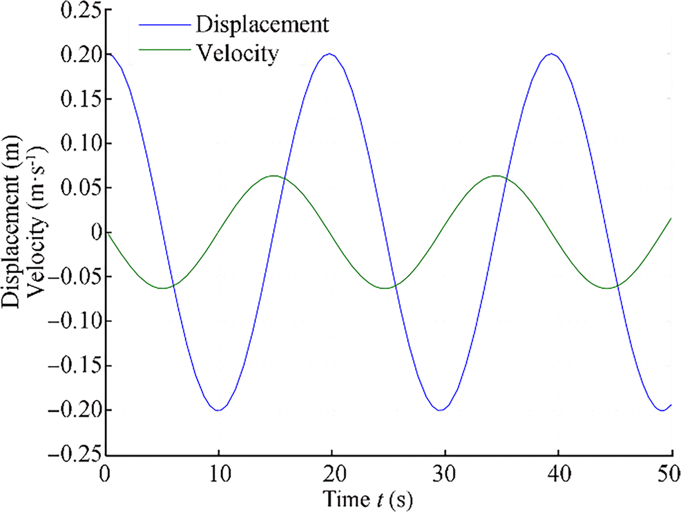Figure  11  Displacement and velocity curves for the oscillator in Example 3 with weak nonlinearity and small-amplitude oscillations

Download: Full-Size Img

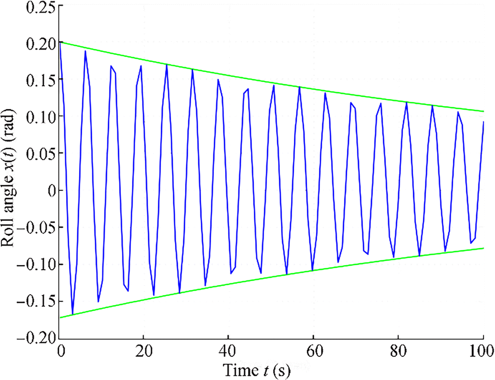Figure  12  Roll angle decay curve with its envelope from Eq. (34)

Download: Full-Size Img

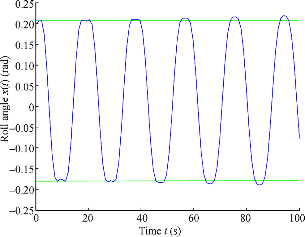Figure  13  Roll angle decay curve with its envelope from Eq. (40)

Download: Full-Size Img

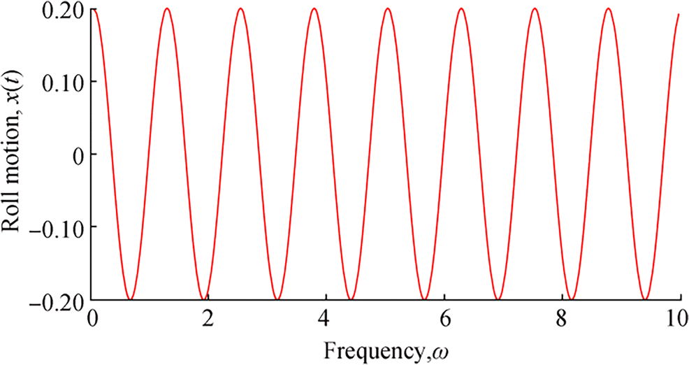Figure  14  Roll motion vs. frequency for Example 3

Download: Full-Size Img

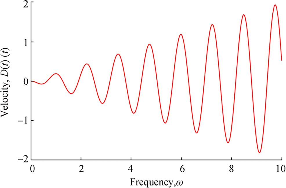Figure  15  Velocity vs. frequency for Example 3

Download: Full-Size Img

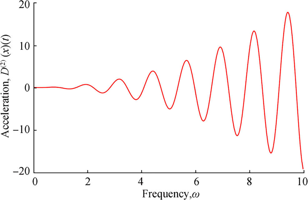Figure  16  Roll motion vs. frequency for Example 3

Download: Full-Size Img

7   Conclusions

In this paper, a mathematical model of the roll motion of ships with nonlinear damping and restoring moments and exciting moments is discussed. To predict the roll motions of ships in irregular or regular waves and to identify the damping and restoring moments in the model, an analytical solution using a modified form of the HPM and a numerical solution using ultraspherical wavelet-based method are obtained. The accuracy of the analytical and numerical solutions is confirmed by a direct comparison with the highly accurate and widely used fourth-order Runge-Kutta method. Analytical expressions for the roll angle, velocity, acceleration, and damping and restoring moments were also derived.

Appendix 1: Ultraspherical polynomials

The ultraspherical polynomials are special types of Jacobi polynomials that are associated with the real parameter $ \left(\alpha \gt \frac{-1}{2}\right) $. They are orthogonal polynomials on the interval (− 1, 1), with respect to the weight function $ w(x)={\left(1-{x}^2\right)}^{\alpha -\frac{1}{2}}, $ and defined by

where

are the eigenfunctions of the following singular Sturm-Liouville equation

The following integral formula and the theorem that follows are needed to establish the convergence of the expansion of the ultraspherical wavelets

Theorem 3 The following inequality holds for ultraspherical polynomials

Appendix 2: Shifted ultraspherical polynomials

The shifted ultraspherical polynomials are defined on [0, 1] by

All properties of ultraspherical polynomials remain valid for the shifted polynomials.

The orthogonality relation for $ {\overset{\sim }{C}}_n^{\left(\alpha \right)}(x) $ with respect to the weight function $ \overset{\sim }{\omega }(x)={\left(x-{x}^2\right)}^{\alpha -\frac{1}{2}} $ is given by

For more properties of ultraspherical polynomials, see Rainville (1960).

Appendix 3: Basic idea of HPM

Consider the nonlinear differential equation

with the boundary condition

where A, B, f(r), and Γ are a general differential operator, a boundary operator, a known analytical function, and the boundary of the domain Ω, respectively. Expressing A(u) as the sum of linear (L) and nonlinear (N) parts, Eq. (74) becomes

The homotopy technique begins by defining

v(r, p) : Ω × [0, 1] → R, such that

where p ∈ [0, 1] is an embedding parameter and u₀ is an initial approximation of Eq. (74) that satisfies boundary conditions (Eq. 75). Evidently, Eq. (77) implies that

As p changes from 0 to 1, v(r, p) changes from u₀ to u_r, a process known as a homotopy. The solution of Eq. (77) may be expressed in terms of a power series in the form:

An approximate solution to Eq. (77) is given by the following: