1   Introduction

Understanding and predicting the behavior of laminar to turbulence transition is one of the important topics in the aerospace and marine engineering. The prediction of the drag force, lift loss, and fluctuations in the pressure field around a body are difficult. Turbulent flow around a geometrically simple and complicated shapes over a wide range of Reynolds numbers has been performed experimentally and numerically. Taneda has experimentally investigated the steady wake behind a sphere at low Reynolds numbers (Taneda 1956). His results indicate that flow around the sphere is perfectly laminar at the Reynolds numbers less than 24. The experimental results indicate that for Reynolds numbers less than 24, the flow around the sphere is perfectly laminar (Taneda 1956). Therefore, there is no flow separation, and the flow stream on the downstream side of the sphere is nearly identical to that on the upstream side (Taneda 1956). Clift et al. (1978) have theoretically studied the drag force acting on prolate and oblate in creeping flow regime. In 1976, characteristics of the steady wake behind a sphere object have been experimentally studied by using the dyed water at the low Reynolds numbers (Nakamura 1976). The existence of a closed recirculating eddy behind a sphere at the Reynolds numbers smaller than 10 has been suggested by Nakamura (1976). The flow passing sphere object at intermediate and high Reynolds numbers have been investigated in detail (Wu and Faeth 1993; Natarajan and Acrivos 1993; Achenbach 1972). An experimental investigation on turbulent flow around a solid ellipsoid using shadow image and digital particle image velocimetry (DPIV) techniques has been carried out by Tokuhiro et al. (1998).

Computational fluid dynamics (CFD) simulations for incompressible fluid flow around ellipsoid at the Reynolds number smaller than 200 have been performed by Taamneh (2011). His results indicate that total drag coefficient around the ellipsoid is strongly dependent on the axis ratio and Reynolds number. Johnson et al. have studied vortex structure in the wake of 2D elliptical cylinder at the Reynolds numbers range of 75 to 175 (Johnson et al. 2004). Their results indicate that by increasing the Reynolds number, the lower frequencies in the far wake play an important role and their inception point occurs closer to the elliptical cylinder.

Pal et al. (2019) have numerically predicted the transport phenomena and Nusselt number distribution of laminar-turbulent annular jets on a surface due to impingement. Their results illustrate that heat transfer from the circular jet is greater than for the annular jet (Pal et al. 2019). Numerical prediction on the heat transfer in laminar and turbulent flows around slot jet by transition shear stress transport model have been carried out by Kadiyala and Chattopadhyay (2017, 2018).

The hydrodynamic forces acting on an ellipsoidal object immersed in the simple shear flow, two-dimensional straining, and axisymmetric straining flow fields have been studied by Blaser (2002). The effects of particle shape on the drag force and drag coefficient have been experimentally and numerically investigated in the literature (Tripathi et al. 1994; Tripathi and Chhabra 1995; Kumar and Kishore 2009). Barberis et al. (1995) have experimentally investigated the three-dimensional separation by considering the flow past a large-scale model consisting of a half-prolate ellipsoid extended by a circular cylinder ending in a flat base at 45^∘ with respect to the cylinder axis. Karlsson and Fureby (2009) have performed Reynolds Averaged Navier Stokes (RANS), detached eddy simulation (DES), and large eddy simulation (LES) models over the flow around a 6:1 prolate spheroid mounted in a wind tunnel with 20^∘ angle-of-attack (Karlsson and Fureby 2009). Chang et al. have analytically and numerically investigated an axisymmetric viscous flow around an ellipsoid of circular section at low Reynolds number by using matched asymptotic expansion and deterministic hybrid vortex methods (Chang et al. 1992). They have also investigated separation angles and wake length for the spheroid. El Khoury et al. have studied flow field around a prolate spheroid at the high Reynolds numbers (≈10⁴) in which major axis of the spheroid was oriented perpendicular to the oncoming flow (El Khoury et al. 2010). The flow field around a sphere has been investigated numerically at subcritical and supercritical regimes by Constantinescu and Squires (2004). The aerodynamic analysis of the spheroid at relatively low angles of attack using two hybrid RANS/LES turbulence models has been numerically studied by Lakshmipathy (2014).

The computations of flow over the spheroid have been performed at two incidence angles of 10 and 20 degrees. Mikulencak and Morris have numerically studied solutions of stationary flow resulting from a single body immersed in a simple shear flow at the different values of Reynolds numbers (Mikulencak and Morris 2004). They have found that the boundary layer separation is observed in the case of fixed cylinder at Re ≈ 85, and for fixed sphere at Re ≈ 100. In this way, laminar-turbulence transition flow around the symmetrical airfoil at the low Reynolds numbers in the free flow and near the ground surface at the different angles of attack has been numerically investigated (Kadivar and Kadivar 2018). Numerical results indicate that by increasing the angle of attack, laminar separation bubbles generated in the free flow are oriented to the leading edge.

There seems to be lack of numerical works on laminar-turbulent transition phenomenon around ellipsoid and prolate spheroid in axisymmetric flow regime and at high Reynolds numbers. Therefore, the aim of this work is to provide a numerical investigation of axisymmetric flow around 2D ellipsoid and 3D prolate spheroid using different turbulence and transition models. The experimental investigation of transition measurement on the DFVLR 1:6 prolate spheroid is used to validate our numerical results. The experimental study has been carried out for axisymmetric flow conditions at different Reynolds numbers in low speed wind tunnel Braunschweig (NWB) by Meier et al. (1987). The wind tunnel has test section of 3.25m × 2.8m. The nominal free-stream velocities U were 15m/s, 40m/s, and 60m/s, giving Reynolds numbers of 1.6 × 10⁶, 6.4 × 10⁶, and 9.6 × 10⁶, respectively. The free-stream turbulence intensity was approximately 12%. Meier et al. have measured turbulence quantities by means of surface hot films in ten different locations on prolate spheroid and interpreted the deviations in the transition locations.

The layout of the rest of the paper is as follows: In Section 2, we will formulate the proper turbulence model for the pressure and velocity fields at the high Reynolds numbers. The numerical procedure to solve the coupled system of partial differential equations for kinetic energies is contained in the Section 3. The results of our numerical solutions, including the distributions of skin friction coefficient on the ellipsoidal surface, are reported in Section 4.

2   Turbulence Model

Turbulence model is a set of differential and algebraic equations which deals with the turbulent transport phenomena. Reynolds Averaged Navier Stokes model is widely applied to handle turbulence phenomena for engineering purposes. Menter has proposed the shear stress transport turbulence (SST) model which is an eddy viscosity model defined as a combination of k − ω model near the boundary layer and k − ϵ model far from the boundary layer (Menter et al. 2002, 2003, 2006). A blending function ensures a smooth transition between the two models. Indeed, the blending function is applied to be one in the near-wall region, which activates the standard k − ω model, and zero far from the wall, which activates the transformed k − ϵ model. Therefore, SST model provides more accurate representation and reliable for wider flow field. The two partial differential equations governing the turbulent kinetic energy, k, and the turbulent frequency ω read (Menter et al. 2002, 2003, 2006):

where μ is the dynamic viscosity, μ_t is the eddy viscosity, u is the velocity field, ρ is the density, and $ {\hat{P}}_k $ and $ {\hat{D}}_k $ are:

where Re_θc is the critical Reynolds number where the intermittency first starts to increase in the boundary layer. y is distance to nearest wall, S is the strain-rate magnitude, and F_θt is blending function used to turn off the source term. P_k is the original production, and D_k and D_ω are original destruction terms from the turbulent kinetic energy equation, respectively. Cd_ω results from transforming the ϵ equation into an equation for ω. The coefficients in the SST model are obtained by combining the value of the coefficients of the standard k − ω (in the near wall region) to those of the k − ϵ model by using the blending function. The modified blending functions are defined as follows:

The transported quantities of the transition model are the intermittency γ and the transition momentum thickness Reynolds number, Re_θt. The intermittency function, γ, is applied to impose the laminar zones and to trigger the transition process by controlling the production term of the turbulent kinetic energy. The transport equation for the intermittency, γ, is defined as:

Transition source, P_γ, and destruction/relaminarization sources, E_γ, are respectively defined as follows:

where Γ is the vorticity magnitude, F_length is an empirical correlation that controls the length of the transition region, and F_onset controls the transition onset location. Both are dimensionless functions that are used to control the intermittency equation in the boundary layer.

The second transport equation for the transport of the transition momentum thickness Reynolds number, Re_θt, (local transition onset momentum thickness Reynolds number) is:

We refer to Menter et al. (2002, 2006) for a detailed description of the model and its parameters. These equations are coupled with Eqs. (1) and (2) of SST turbulence model and constitute a coupled systems of partial differential equations which yields velocities, pressures, turbulent kinetic energy, turbulent dissipation, and finally local state of transition conveyed by γ and R_θt.

3   Numerical Approach

The numerical method is based on finite volume method which is adopted to solve the Reynolds Averaged Navier Stokes (RANS) equation. The left, right, and bottom boundaries of the domain are modeled respectively as velocity inlet flow, pressure outlet flow, and axis boundary. The boundary conditions and boundary layer grid are depicted in Figure 1. Figure 1 illustrates the 2D meshing and 3D meshing of the ellipsoid.

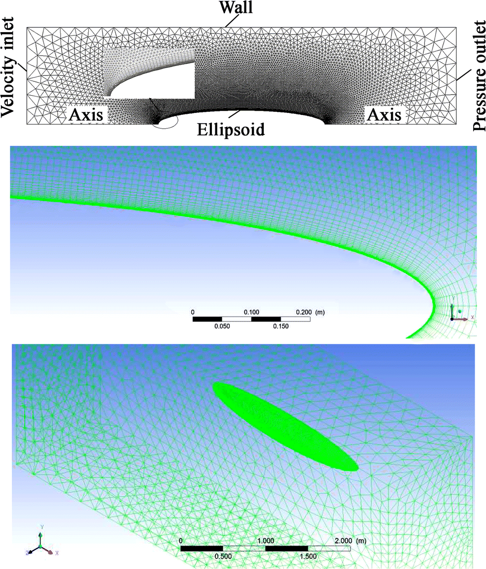Figure  1  View of the computational domain with boundary layer region, free-stream region, and two-dimensional and three-dimensional meshes of the ellipsoid

Download: Full-Size Img

In order to obtain the appropriate grid, several meshes with different element were generated, and the obtained results were compared. The transition phenomenon depends on accurate resolution of the boundary layer near the surface of the body. To predict accurate transition onset, the construction of grid and the computational domain for model are divided into two sections. These two sections are boundary layer region and the free-stream region. In this way, high-quality elements are produced in regions where the fluid is subject to large gradients. The grid independence is achieved with the comparison of different grid cell sizes. It was found that about 27 000 cells for 2D ellipsoid and 1 362 460 cells (including 897 120 wedge grids and 465 340 tetrahedral ones) for 3D spheroid are satisfactory, and any increase beyond this mesh size would lead to insignificant changes in results. In order to find the laminar and transition boundary layers, the grid must have a y⁺ less than one, because the transition onset moves upstream with increasing y⁺. The distance from the wall is so selected to give y⁺ less than one.

The numerical investigations of flow around airfoil have been done by commercial Ansys FLUENT 15 software. The 2D formulation of RANS equations has been solved using different turbulence models of Spalart-Allmaras (Spalart and Allmaras 1994), k − ω SST (Menter et al. 2002, 2003, 2006), and SST-Trans (Menter et al. 2004). Second-order discretization has been selected for the continuity, momentum, and turbulent variables. The gradient evaluation has been performed with a node-based method. The pressure-velocity coupling has been calculated using SIMPLEC algorithm.

4   Results and Discussions

4.1   Two-Dimensional Modeling

In this section, we numerically study the laminar-turbulence transition flow around a two-dimensional ellipsoidal by applying the different turbulence models. To find a proper turbulence model for the prediction of the laminar-turbulence transition, we compare the results of different turbulence models with experimental results (Meier et al. 1987) which were reported at the same Reynolds numbers.

All of the obtained results for the different turbulence models including k − ω SST, SST-Trans, and Spalart-Allmaras models were calculated using the commercial Ansys FLUENT 15 software. The skin friction coefficient equation is defined by:

where τ_w is wall shear stress and q_∞ is free-stream dynamic pressure. The results of skin friction measurements as a function of free-stream Reynolds number, based on the length of model obtained on the ellipsoid at zero incidence for different turbulence models, are shown in Figures 2, 3, and 4. Figures 2, 3, and 4 illustrate the skin fraction coefficient distributions for different Reynolds numbers and ten different positions on the ellipsoid calculated on the basis of k−ω SST model, Spalart-Allmaras model, and SST-Trans model, respectively. As one can observe in Figures 2 and 3, k−ω SST model and Spalart-Allmaras model are not able to predict the laminar-to-turbulent boundary layer transition.

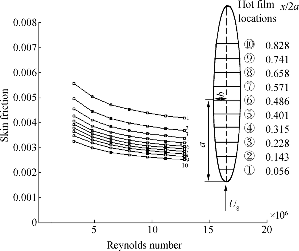Figure  2  Profiles of skin friction coefficient distributions computed by k-ω SST model as a function of Reynolds numbers at ten positions of the ellipsoid

Download: Full-Size Img

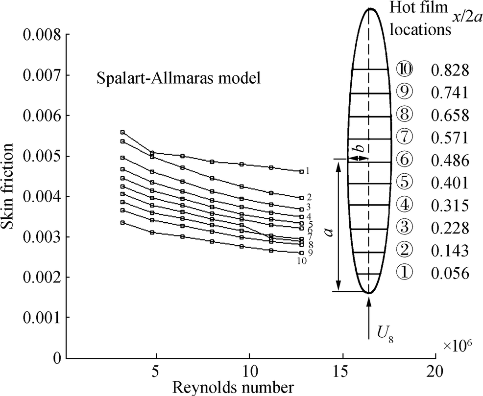Figure  3  Profiles of skin friction coefficient distributions calculated from Spalart-Allmaras turbulence model as a function of Reynolds numbers at ten positions of the ellipsoid

Download: Full-Size Img

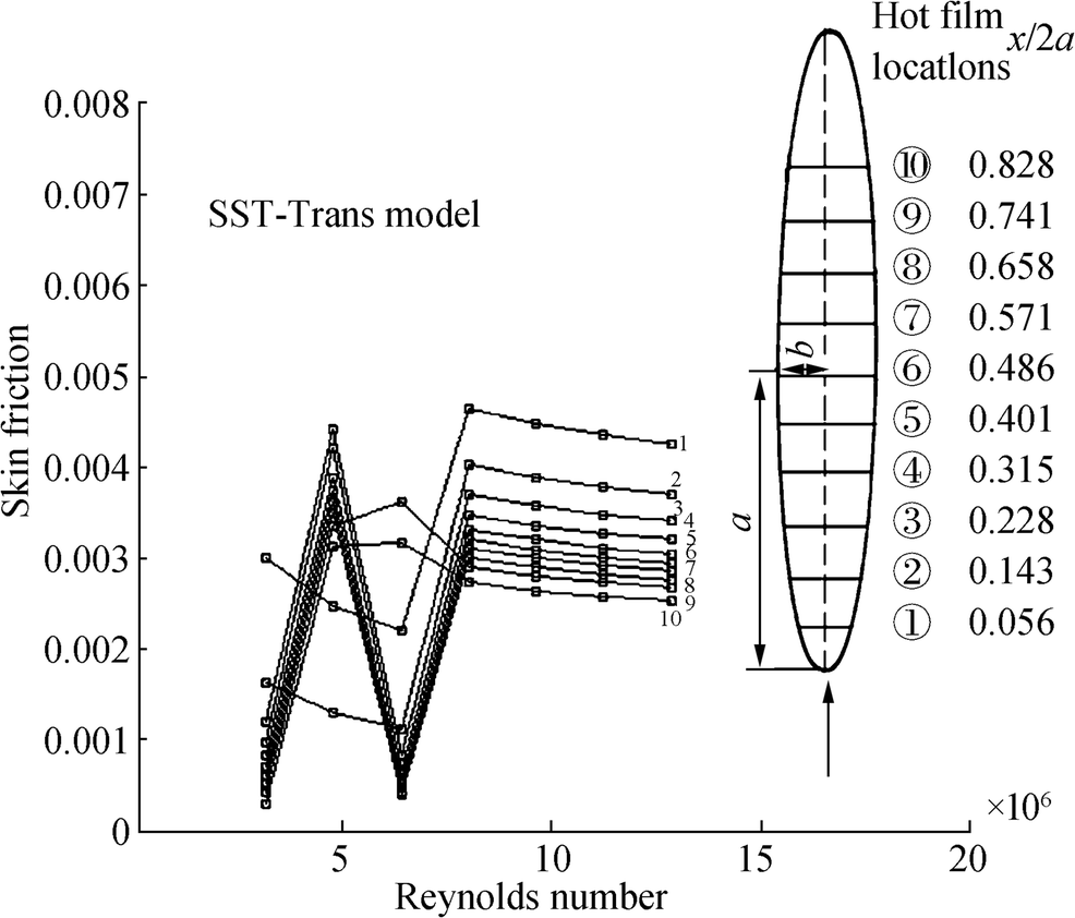Figure  4  Skin friction coefficient distributions calculated using SST-Trans turbulence model as a function of Reynolds numbers at ten positions of the ellipsoid

Download: Full-Size Img

Figure 4 illustrates the laminar-to-turbulent boundary layer transition region which is clearly indicated by increase of the skin friction coefficient distributions. It can be observed that the first increase of the wall shear stress or the strong increase of the skin friction coefficients identifies the laminar-turbulent transition onset.

Figure 5 shows the skin fraction calculated using SST-Trans as function of ellipsoid length for different Reynolds numbers. Our numerical results indicate that for the Reynolds numbers of 1.6 × 10⁶ and 6.4 × 10⁶, the transition onsets are presented respectively at x/2a = 0.89(x = 2.136m) and x/2a = 0.67(x = 1.608m). As can be seen in Figure 5, SST-Trans model cannot predict the laminar-to-turbulent transition on the two-dimensional ellipsoidal above the Reynolds numbers of Re = 6.4 × 10⁶.

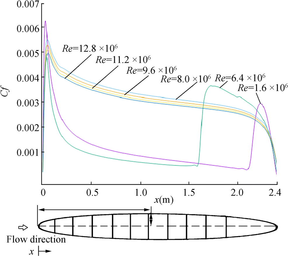Figure  5  Profiles of skin friction coefficient distributions calculated using SST-Trans turbulence model as a function of ellipsoid length for different Reynolds numbers.

Download: Full-Size Img

In order to test the validity of the numerical results, the numerically calculated skin friction coefficient distributions as a function of length of ellipsoid were compared with the experimentally measured data obtained at the same experimental conditions on Figure 6. The experimental data has been carried out for axisymmetric flow conditions at different Reynolds numbers in low speed wind tunnel Braunschweig (NWB) by Meier et al. (1987). The wind tunnel has test section of 3.25m × 2.8m. The nominal free-stream velocities U were 15m/s, 40m/s, and 60m/s, giving Reynolds numbers of 1.6 × 10⁶, 6.4 × 10⁶, and 9.6 × 10⁶, respectively. The free-stream turbulence intensity was approximately 12%. As one can see in Figure 6, although the SST-Trans model is able to predict turbulent boundary layer transition, but the predicted transition location is about 50% off from the experimental measurements. It means that the SST-Trans model is not good enough to describe turbulent boundary layer transition on the 2D ellipsoid. Therefore, we will apply SST-Trans model for the prediction of the transition onset in three-dimensional ellipsoid.

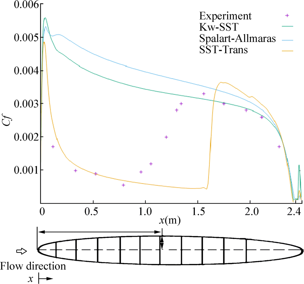Figure  6  Comparison of experimental data from prolate spheroid test case skin friction coefficient distribution obtained by the experimental work of Meier et al. (1987) with different turbulence models. Numerical and experimental data are as follows: U_∞ = 40m/s (Re = 6.4 × 10⁶), a = 1.2m, and b = 0.2m

Download: Full-Size Img

4.2   Three-Dimensional Modeling

In this section, we employ SST-Trans turbulence model to numerically investigate the laminar-to-turbulent transition for three-dimensional prolate spheroid with an aspect ratio of a :  b = 1.2 :  0.2 = 6 :  1 where a is the length of the major axis and b is the length of the two minor axes. Figure 7 illustrates the velocity vector field around the 3D ellipsoid by vectors, in the longitudinal symmetry plane.

Figure  7  Velocity field around the three-dimensional ellipsoid. a) U = 10 m/s, b) U = 30 m/s, c) U = 40 m/s, and d) velocity field in the small recirculation zone around the ellipsoid

Download: Full-Size Img

To validate the consistency of the numerical model, we compare the skin friction coefficient distribution reported by Meier et al.'s experimental data with the simulated ones which were obtained using the same condition of Reynolds number. Figure 8 illustrates the comparison of the skin friction coefficient distribution against the ellipsoid length for Reynolds number Re = 6.4 × 10⁶. The experimental data were extracted from the Meier et al.'s work (Meier et al. 1987). The experimental data indicates that for Reynolds number of Re = 6.4 × 10⁶, the laminar-turbulent transition point is x/2a = 0.401(x = 0.962m). SST-Trans prediction of laminar-turbulent transition location is about x/2a = 0.390(x = 0.936). There is a very good agreement between experimental and numerical results of skin fraction coefficient at the Reynolds number of 6.4 × 10⁶ as shown in Figure 8.

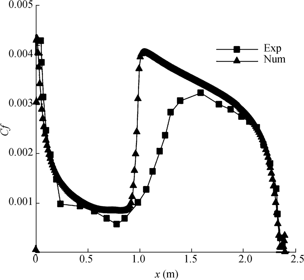Figure  8  Skin friction coefficient distribution against the ellipsoid length at a given value of Reynolds number of Re = 6.4 × 10⁶. The solid square were extracted from the experimental data [25], and the solid triangles correspond to our numerical results from 3D SST-Trans model at U = 40 m/s (Re = 6.4 × 10⁶)

Download: Full-Size Img

Figure 9 illustrates the comparison of the numerically calculated skin friction coefficient with the experimental data at the three different values of Reynolds number. A good agreement has been found between experimental results and our numerical data. The percentage difference between experimental and computed laminar-turbulent transition point is less than 12% for Reynolds numbers of 9.6 × 10⁶.

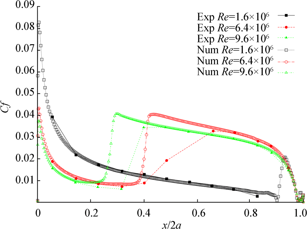Figure  9  Comparison of experimental data and numerical results of skin friction coefficient 6:1 spheroid at different values of Reynolds number

Download: Full-Size Img

Figure 10 indicates the distribution of skin friction coefficient on the three-dimensional ellipsoid as a function of ellipsoid length for different Reynolds numbers. The numerical results were obtained from the three-dimensional SST-Trans turbulence model. Our numerical results indicate that by increasing the Reynolds number, the laminar-turbulent transition point moves towards the leading edge of spheroid surface.

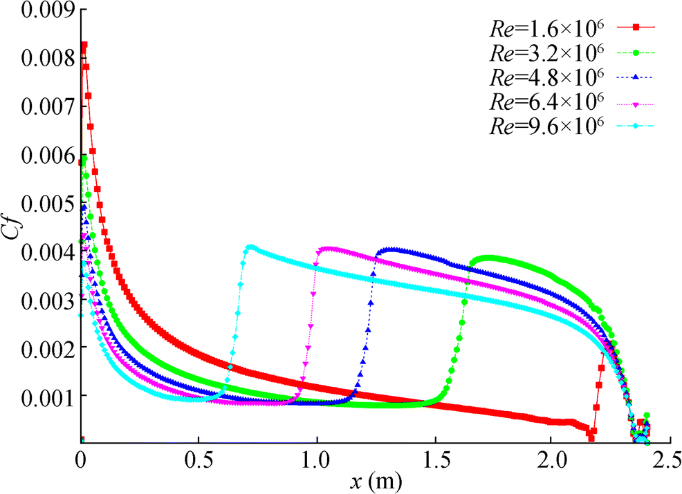Figure  10  Distribution of skin friction coefficient on the 6:1 prolate spheroid as a function of ellipsoid length at the different values of Reynolds number

Download: Full-Size Img

Figure 11 illustrates the behavior of skin friction coefficient as a function of Reynolds number at different position of ellipse. As one can see, SST-Trans prediction of skin friction coefficients illustrates that by increasing the Reynolds number, the laminar-turbulent transition onset location moves towards the leading edge of spheroid.

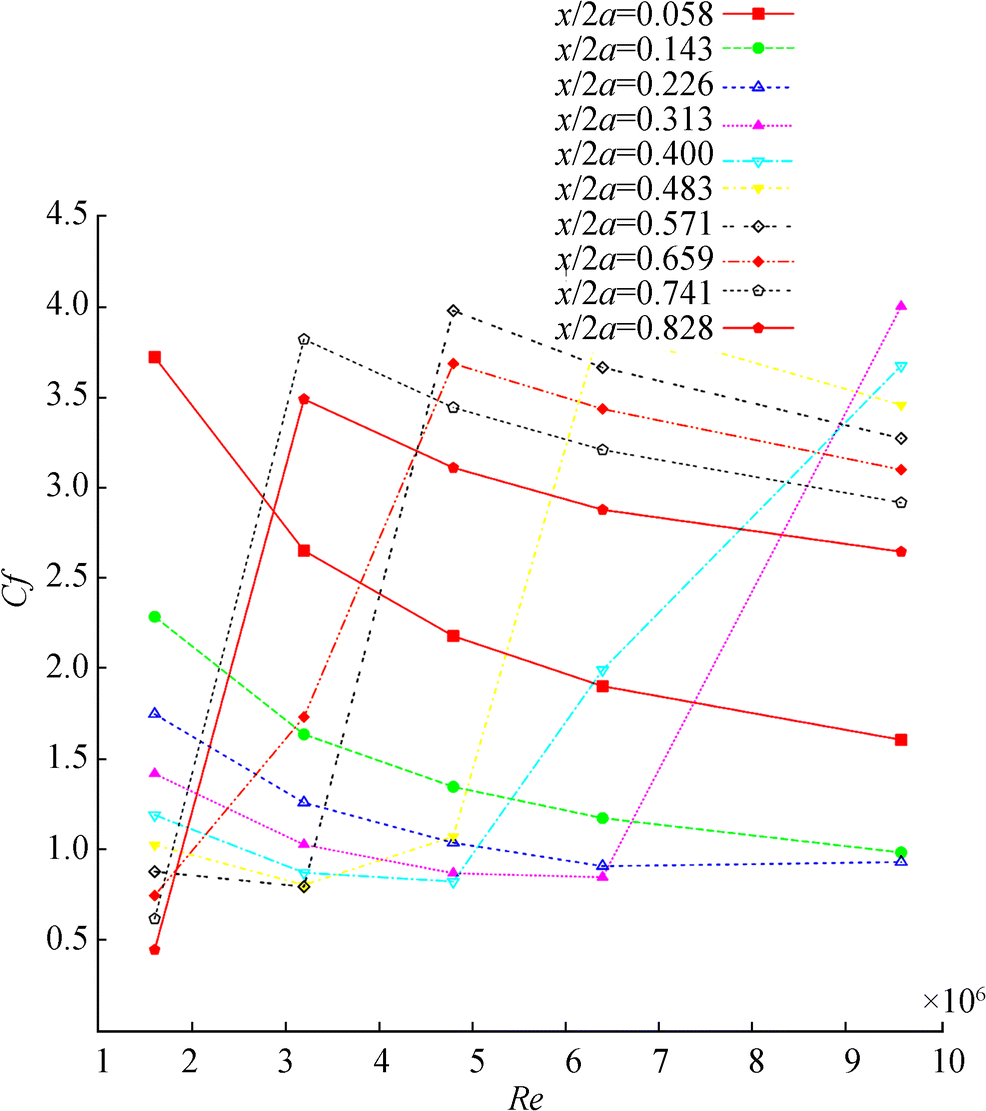Figure  11  Skin friction coefficient distributions calculated using three-dimensional SST-Trans turbulence model as a function of Reynolds numbers at the ten positions of 6:1 prolate spheroid

Download: Full-Size Img

5   Conclusion

In this work, the laminar-turbulent transition phenomenon around the two- and three-dimensional ellipsoid at the high Reynolds number has been numerically investigated. The k−ω SST, Spalart-Allmaras, and SST-Trans models have been used to perform RANS simulations. Our numerical results indicate that k−ω SST model and Spalart-Allmaras model are not able to predict the laminar-to-turbulent boundary layer transition on the ellipsoid surface. The results of SST-Trans prediction were validated with experimental data measured at the same values of Reynolds number. A good agreement has been observed between the experimental and the numerical data, when comparing the laminar-turbulent transition location.