1   Introduction

Corrosion and fatigue cracking may be the two most important types of damage in ageing ship structures, which lead to surface roughness, reduction of the plate thickness and strength and eventually to leakage and structural failure.

Corrosion in ship structures has an essential role in long-term structural integrity. Under conditions of high temperature, improper ventilation, high stress concentration, high stress cycling, very high rates of corrosion can be achieved in spaces such as ballast tanks and at specific structural details such as horizontal stringers or connections of longitudinal stiffeners and web frames. This has been a source of concern by ship operators, and Classification Societies that have collected much service data (TSCF 1992, 1997; Wang et al. 2003; Yamamoto and Ikagaki 1998). Corrosion has clear consequences in degrading the ultimate strength of ship structures (Jiang and Guedes Soares 2012; Nakai et al. 2006; Paik et al. 2003; Silva et al. 2013) and also in affecting the fatigue strength by increasing the stress levels (Garbatov et al. 2002; Guedes Soares and Garbatov 1998; Moan and Ayala-Uraga 2008; Tran Nguyen et al. 2012, 2013) and also by a direct degradation of fatigue strength (Garbatov 2016; Garbatov et al. 2014a).

Fatigue is an important design criterion for locally welded structural components and global structures. The fatigue damage may even further reduce the strength because of the presence of different imperfections, which can lead to a local increase of stresses and fatigue crack initiation and propagation. For fatigue life assessments, different procedures have been developed based on databases of the fatigue behaviour of welded structural components as a result of both tests and theoretical investigations (Fricke and Petershagen 1992).

The main steps in fatigue analysis are based on direct calculations that involve the description of the wave-induced loading (Guedes Soares and Moan 1991) the stress distribution in the structure (Guedes Soares et al. 2003), the model of fatigue damage (S-N approach) or fracture mechanics approach (Paris and Erdogan 1963) and the probabilistic evaluation of the different steps to arrive at a safety index or time-dependent reliability as has been developed in Guedes Soares and Garbatov (1999). The analysis of stresses is a difficult task due to the complexity of the ship structures. Nowadays, the methods that are mostly accepted and spread for analysing complex welded structures are the hot spot stress approach (Petershagen et al. 1991) and the effective notch stress approach (Radaj 1990; Radaj et al. 2009). Recommendations for fatigue stress assessment can be found in guidelines (Niemi 1992, 1995; Niemi et al. 2004).

The work presented here is analysing small-scale specimens of a transversely stiffened welded plate, which were firstly corroded and then fatigue tested. The surfaces of 11 corroded specimens are analysed applying photogrammetry techniques to obtain the 3D geometrical description of the corroded surfaces. The description of fatigue tests, together with results and statistics of the corroded surfaces, is given in Garbatov et al. (2014a) and Garbatov et al. (2014b).

In the present study, the relations between the statistical properties of the corroded surfaces of the specimens and the experimentally estimated stress concentration factors (SCFs) are investigated. Finite element (FE) analyses, using very fine 3D elements, have been performed on the idealised finite element models of corroded specimens to estimate the SCFs. To determine an appropriate mesh density, the convergence study is performed. SCFs calculated by the finite element method (FEM) are then compared with the ones estimated experimentally, and their dependency on statistical properties of corroded surfaces is investigated. The correlation between actual and predicted crack locations is also calculated and discussed.

2   Fatigue Test Setup

The fatigue specimens have been cut from box girders that have been subjected to corrosion, in a real corrosive environment in direct contact with seawater. The dimensions of the box girder specimen were 1400 × 800 × 600 mm. The box girder was made of standard shipbuilding steel with a yield stress of 235 MPa. The box girder specimen was exposed to the Baltic seawater and tested in hot water. The box girder was placed in a large tank, and seawater was pumped into the tank continuously. The temperature of seawater was increased and additionally, oxygen depolarisation sub process rate was increased by the agitation of seawater, which resulted in a corrosion rate increase.

The test duration was 90 days without polarisation. More detailed information about the corrosion set up may be seen in Domzalicki et al. (2009). The total weight loss observed was 56 kg (23% of initial weight). The average value of the electrolyte flow rate was 308 dm³/h; water temperature was 45.2 ℃ and pH = 7. 93.

After the test was completed, the box girder was covered with iron corrosion products. This box girder has been subjected to ultimate strength tests as described in Saad-Eldeen et al. (2011, 2013a, b). Eleven fatigue test specimens were cut from the box girder in a shape that can be seen in Figure 1 (Garbatov et al. 2014a).

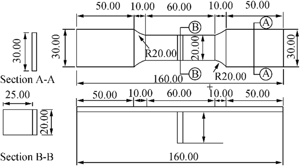Figure  1  Fatigue test specimen configuration

Download: Full-Size Img

The non-corroded thickness of specimens was 4.5 mm. To accurately characterise the test specimens, an analysis of their thickness has been made employing photogrammetry techniques. The corroded specimens were scanned with an optical 3D scanner (Atos III Triple Scan, GOM mbH, Germany). The geometries were reconstructed using Geomagic Spark (3D Systems, USA) software, and the thickness of the specimens was determined using GOM Inspect (GOM mbH, Germany) software packages (see Figure 2). The minimum, maximum, mean value and standard deviation of corroded specimen thicknesses are given in Table 1 (Garbatov et al. 2014a).

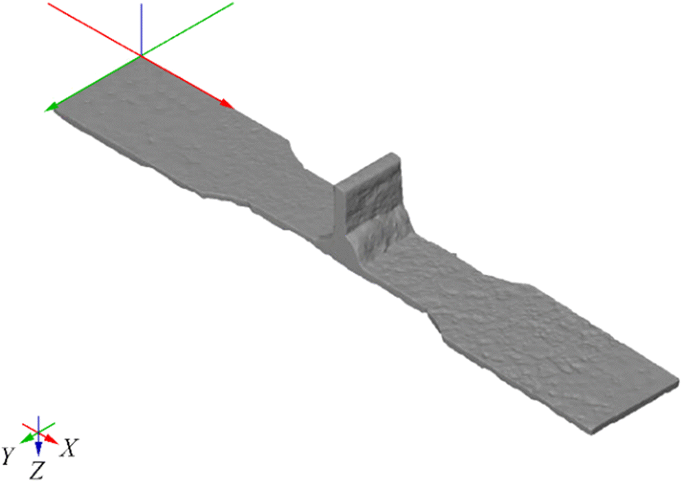Figure  2  Scanned corroded specimen

Download: Full-Size Img

The corroded specimens (see Figure 1) were fatigue tested to axial cyclic load (Garbatov et al. 2014a). A transverse stiffener is welded to one side of the specimen. The specimens are not symmetrical about the load axis. The design of the specimen assumes that if the specimen is intact, without corrosion, the failure occurs along the toe of the transverse fillet weld.

Eleven specimens with different corrosion degradation levels are used to analyse the effects of the degradation and to evaluate the fatigue performance. Figure 1 shows the dimensions of specimens. All specimens were 180 mm in length and had a plate thickness of intact non-corroded specimen of 4.5 mm. The stiffener of intact non-corroded specimen was also 4.5 mm thick. The stiffener width was 17.6 mm. The specimens were welded based on regular shipyard practice and were machined to smooth the edges.

All specimens were tested under cyclic loading at a nominal stress range, Δσ as shown in Table 2. The stress range is the difference between the minimum and maximum nominal stresses. The stress range across the net section of the plate, which varies from specimen to specimen as can be seen in Table 2, is modelled as 120, 155 and 200 MPa, respectively. These nominal stresses were calculated by dividing the applied axial load on the specimen by the mean cross-sectional area of the plate. The lower stress limits correspond to 6, 8 and 11 MPa, respectively, whereas the upper-stress limit was 126, 163 and 210 MPa, respectively. It should be noted that the three groups of loading have been simulated A, B and C. The first group consists of specimens 6, 7, 8 and 10, the second group covers the specimens 9, 14 and 17 and the third one includes 4, 11, 12 and 13 (Figure 3).

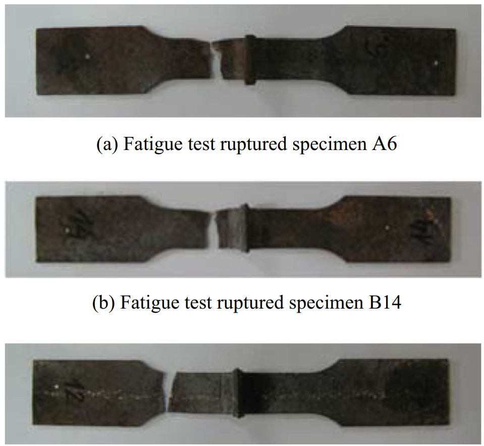Figure  3  a Fatigue test ruptured specimen A6. b Fatigue test ruptured specimen B14. c Fatigue test ruptured specimen C12

Download: Full-Size Img

All samples were tested to failure, and typical crack locations are shown in Figure 3. It has been observed that all of the failures initiated at a specific corrosion pit at the narrowed plate away from the fillet weld due to severe corrosion in the specimens. None of the specimens failed at the weld toe, although this was expected before performing experiments.

3   Fatigue Strength and SCF Analysis

The fatigue life, or several loading cycles to failure, was recorded and presented for each specimen in Table 2. A very large scatter of fatigue life can be observed. Fatigue life data exhibit widely scattered results because of inherent microstructural inhomogeneity in the material properties, differences in the surface and material properties due to corrosion.

3.1   Experimentally Estimated SCFs

To estimate the SCF experimentally, the S-N curve is defined as

where Δσ is the stress range, N the number of cycles to failure while m and K₅₀ are the constants depending on the type of welded connection. The index "50" denotes the mean S-N curve, i.e. for the stress range level Δσ, the specimen fails with a probability of 50%. The stress range, for a given number of cycles to failure N, can be calculated using Eq. (1) as

The S-N curve used in the present study for the assessment of the specimens, excluding any stress concentration, is the category "B" curve as defined by the UK Department of Energy (BV 1996). The curve is valid for non-tubular joints in as-rolled condition with no flame-cut edges, and the constants m = 3 and K₅₀ = 1.342 × 10¹³ characterises it. The stress range calculated by Eq. (2) is to be multiplied by factor 1.45 representing the ratio of fatigue strength of a smooth specimen to that of the plates in the as-rolled condition (BV 1996):

where Δσ_AR represents a stress range of as-rolled specimen given by Eq. (2). The factor 1.45 is taken as stipulated in BV (1996) as a ratio of the fatigue strength of a smooth specimen to as-rolled one. The B-class refers to as-built specimen, while the strength of the smooth specimen is 1.45 times higher.

The SCF of each corroded specimen may then be experimentally defined as a ratio of stress range, Δσ_SS calculated by Eq. (3), for the number of cycles of the fatigue life of the corroded specimens as is given in Table 3, to the stress range, Δσ, which represents the nominal stress range used during the fatigue test of the corroded specimen as specified in Table 3:

Thus, the SCFs, as calculated by the described procedure, are given in Table 3. As a consequence of highly scattered fatigue lives, the SCFs presented in Table 3 also exhibit widely scattered results.

3.2   SCF Dependency

The dependence of the experimentally estimated SCFs (see Table 3) on several relevant statistical parameters of the corroded specimens is investigated here. Thus, a linear regression analysis concerning the maximum, minimum, mean and standard deviation of the measured thickness is performed. The results of the dependency analysis are presented in Figure 4.

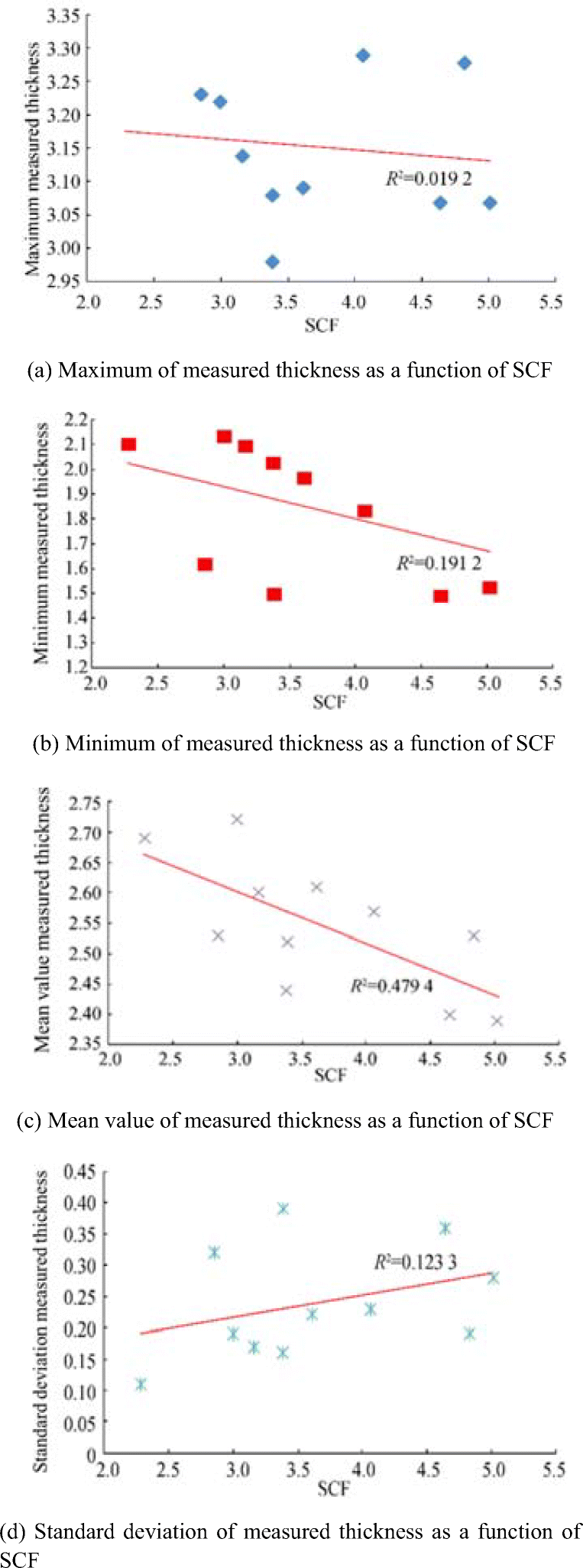Figure  4  a Maximum of measured thickness as a function of SCF. b Minimum of measured thickness as a function of SCF. c Mean value of measured thickness as a function of SCF. d Standard deviation of measured thickness as a function of SCF

Download: Full-Size Img

The adequacy of the linear regression is estimated by the coefficient of determination R², which is approaching 1 in the case of a perfect correlation between the regression model and measured values. As can be seen from Figure 4, a large scatter around the trend is observed and the only acceptable dependency is the one between the mean value of the thickness of the corroded specimen and the SCFs as R², in that case, is 0.480. For all analysed parameters, except for the standard deviation, as the thickness goes down, the SCF grows, which may be explained by the fact that the corrosion pits become more in-depth and sharper leading to shorter fatigue lives. In the case of the standard deviation, as the corrosion degradation develops the standard deviations grow much faster than the mean value of the corrosion depth indicating a bigger scatter around the trend. For the much more corroded plates with a small resulting mean value of the corroded thickness, the observed standard deviation is more significant than for the one with lower corrosion degradation. This fact is also confirmed by Figure 4, where for a smaller mean value and more significant standard deviation of the corroded thickness, the SCF is bigger.

It must be clarified that the average thickness is the most relevant parameter because it is associated with the stress levels in the specimen. However, the average thickness was estimated from measurements before the experiments were performed, and the imposed force is adjusted to have approximately the target average stress level in the specimen (see Table 2). Increasing SCF with decreasing mean thickness is, therefore, a consequence of the fact that higher corrosion wastage is correlated with more frequent, more in-depth and sharper pits.

4   Finite Element Analysis of SCF

To investigate the SCFs of the corroded specimens, an FE analysis of the idealised geometries of the corroded specimens is performed using ABAQUS software. FE models are built based on the scanned geometries obtained in STL format. Surfaces are reconstructed using GeoMagic Spark software with the support of ProEngineer software. Finally, STP files are generated by closed volumes. The typical STP geometry of a specimen is presented in Figure 5.

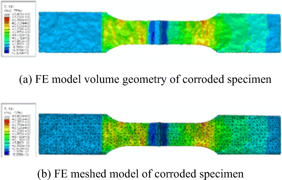Figure  5  a FE model volume geometry of corroded specimen. b FE meshed model of corroded specimen

Download: Full-Size Img

The boundary conditions of the FE model are imposed to represent actual constraints of the specimen during the fatigue testing. One end of the specimen is completely fixed, while axial forces are imposed on the other end of the model. The magnitude of the imposed nominal stress in the cross-sectional area of the narrow part of the specimen is 1 MPa. The estimated average cross-sectional area of each specimen is taken into account, so the axial force is adjusted to reflect differences in the average corrosion wastage between individual specimens.

In the shipbuilding industry practice, the total stress at the anticipated crack location of the weld toe is calculated as (Parunov et al. 2013)

where σ_nom is the nominal stress, calculated either by simple beam theory either by the coarse-mesh finite element analysis. The hot spot stress concentration factor, K_s, takes into account the effect of structural discontinuities and K_w is a notch factor. The product of the nominal stress σ_nom and stress concentration factor K_s (Δσ_hs = K_sΔσ_nom) is known as the hot spot σ_hs or the structural stress. Ship classification societies establish a strict procedure on how to calculate this stress that includes standardisation of mesh size, finite element types and stress extrapolation (DnV 2010). The non-linear stress increase at the local notch is taken into account by the notch stress concentration factor K_w. In the fatigue analysis of ship structural details, K_w is usually proposed as a pre-defined factor, rather than requiring a very detailed finite element analysis. A difficulty raised with the calculation of the notch stress is that a 1 mm fictitious notch rounding should be modelled to estimate the stress increase at the weld toe. Consequently, a very fine mesh with an element size of 0.25 mm would be required.

In the present case of analysis of corroded specimens, the resulting SCF includes both types of stress concentrations. Pitting holes, irregularly distributed along the specimen surface, produce a structural discontinuity that causes stress concentrations. Although those places of stress concentration are away from the sharp corners, they have a similar notching effect as has a weld toe of intact non-corroded structural detail. Therefore, the calculation method employed should be capable of taking into account both types of stress concentration. Presently, there is not an approach standardised by either classification societies or other bodies interested in fatigue assessment of corroded structures (e.g. Haagensen and Maddox 2013; Hobbacher 2009). The present study aims to check the results of applying a 3D solid model with very fine mesh to model the corroded specimens with pits. This is possible nowadays due to the highly developed computing techniques and corresponding FE software solutions.

The analysis is subdivided into three tasks—firstly, a convergence study is performed on one of the specimens to identify the trends and the accuracy of results vs element size. The second step of the analysis is to estimate the SCFs of each specimen numerically and to compare with experiment, while the third task is to perform a comparative study of the regions of high stress concentrations from FE analysis and locations where the crack propagation was observed during the experimental fatigue test. The crack initiation starts in different locations for the fatigue tested specimens. This is explained by the fact that the surface roughness and pit penetrations are non-uniformly distributed and in all of the cases the crack initiation is not colliding with the weld toe hotspot, which usually occurs for the intact non-corroded specimens.

Principal stresses are recommended by ship classification societies for fatigue assessment (BV 1996; DnV 2010); therefore, the significant principal stresses are employed in the present study. However, the choice of some other stress components may be discussed as well. Tetrahedral elements of the second order with ten nodes (C3D10) are used in the modelling. Although hexahedral elements are the preferred element type regarding the accuracy of results, because of the slightly irregular shape of the surface, tetrahedral meshing could not be avoided.

The convergence study is performed for the specimen C4 (Table 1). Six models with a progressively increasing number of elements are used, while the measure of the convergence is the displacement of the free edge of the specimen and the maximum SCF. Finite element models 1 (18, 042 elements), 2 (61, 285 elements), 4 (1, 213, 217 elements), and 6 (1, 564, 573 elements) are presented in Figure 6, where the colours represent principal stresses.

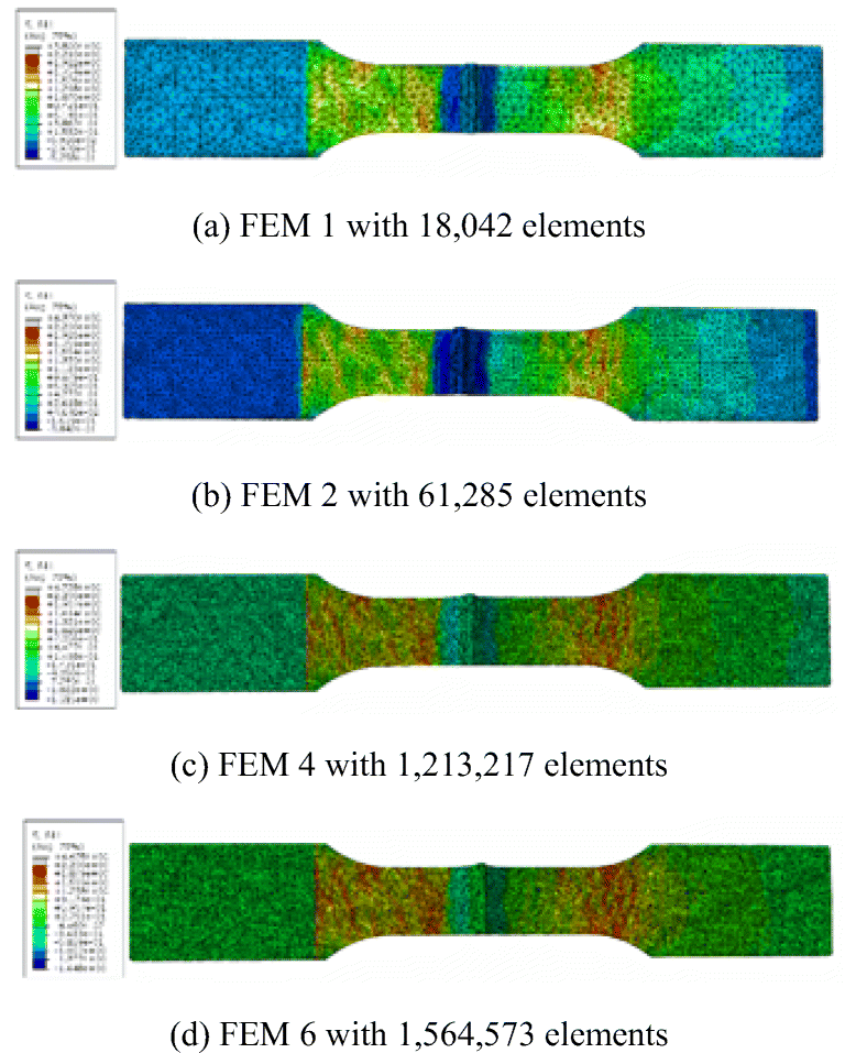Figure  6  Finite element models with coarse a, medium b and fine c meshes

Download: Full-Size Img

The number of finite elements used, several nodes, the typical length of the element edge and estimated maximum displacements and maximum SCF are given in Table 4 and Figure 7.

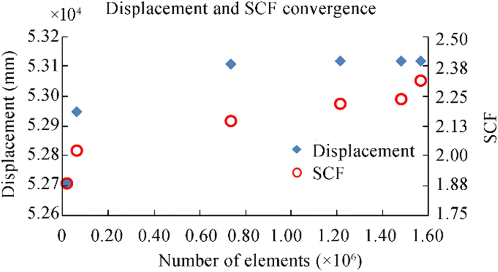Figure  7  Displacement and maximum SCF as a function of the number of elements in FEM

Download: Full-Size Img

As can be seen from Table 4 and Figure 7, the displacement convergence is achieved for the model 3, (734, 931 elements and 1, 074, 280 nodes). The convergence concerning the stresses is quite more complicated. Refining the element size, the maximum stresses are increasing, and they also appeared in different locations. As may be seen from Table 4 and Figure 7, the convergence of the maximum SCFs is also achieved for model 3 if the precision of the SCF is kept to one decimal place, with differences of about 5% in model 6. Such a level of accuracy may be assumed to be acceptable for the present study.

Accounting for the fact that the displacement and SCF convergence was well achieved for the FE model 3, FE model 4 (1, 213, 217 elements and 1, 751, 270 nodes) is considered as a reasonable and safe choice for the SCF analysis of the remaining corroded specimens. Finer models are not considered to be practical as the computational cost is increasing without providing substantially different results. Therefore, in the analysis of SCFs, the typical length of the element used in the modelling reads 0.4 mm (Table 4).

5   Comparative Analysis of SCF of Corroded Specimens

The experimental SCF is defined as a fictitious one, based on the number of cycle of the experimental fatigue life and the nominal stress range of the average corroded plate thickness. The stress range and number of cycles to failure relationship are defined as

where Δσ_notch^m is the notch stress estimated as

where the nominal stress range, Δσ_nom is as input data for the experiments (Table 2). K₅₀ and m are given for the B S-N curve from the UK Department of Energy, where 1.45 is a factor taking into account that the B-curve includes "as-rolled", instead of a smooth specimen. The smooth specimen could have 1.45 higher fatigue strength (BV 1996).

The finite element analysis of the remaining specimens is performed using an FE model corresponding to the length of elements of 0.4 mm. The results of the FE analyses are presented in Table 5 and Figure 8, together with the experimentally estimated SCFs.

Figure  8  SCFs estimated experimentally and by FEA

Download: Full-Size Img

If the modelling error is defined as Φ = SCF_FEM/SCF_Exp, then the mean value of Φ reads 1.00, while its standard deviation is 0.30. It may be stated that on average, the numerically estimated SCFs calculated by FEA predict the experimental SCFs accurately, while the dispersion of the predictions measured by standard deviation is rather large. However, it has to be pointed out that the experimentally estimated SCFs also have dispersion, which is of a comparable order of magnitude as the dispersion of Φ, then one may conclude that the numerical predictions of SCFs are reasonably accurate.

To further analyse the SCF estimates, the dependency of numerical SCFs on statistical properties of the corroded surface is determined and presented in Figure 9.

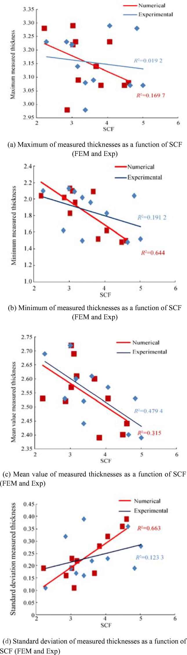Figure  9  Statistical descriptors of measured thicknesses

Download: Full-Size Img

It can be observed in Figure 9 that the coefficients of determination R² are generally much higher for the SCF estimated by FEA than for the ones experimentally estimated. The only regression trend line that shows somewhat lower R² for SCF_FEM than the one for SCF_Exp is on the mean value of corroded plate thickness. However, those two trend lines are almost identical, and they both present quite a clear trend of increasing SCFs with a reducing of the mean value of corroded plate thickness.

It is interesting to compare the actual failure location with areas of high stress concentrations calculated by FEA. As already elaborated, it is not always an easy task to establish such relationship as increased stress concentration in FE models is obtained in different locations, very often also on opposite sides of the model. Furthermore, SCFs observed at different locations are often reasonably close indicating various potential positions of the crack initiation and propagation. Therefore, careful analysis of stresses is necessary to establish a correlation with failure from the experiments. Typical situations are shown in Figure 10 for specimens C11 and B14. In the case of specimen C11, the stress concentration is visible in several locations along with the specimen. However, the stresses at the left upper transition from narrow to the wide part of the specimen are responsible for the failure. The FEM quite well predicts failure location. For the specimen B14, the predicted failure location is at the bottom of the specimen, not far away from the weld toe. Although there are other areas of elevated stresses in the FEM, the failure location is well predicted also in this case.

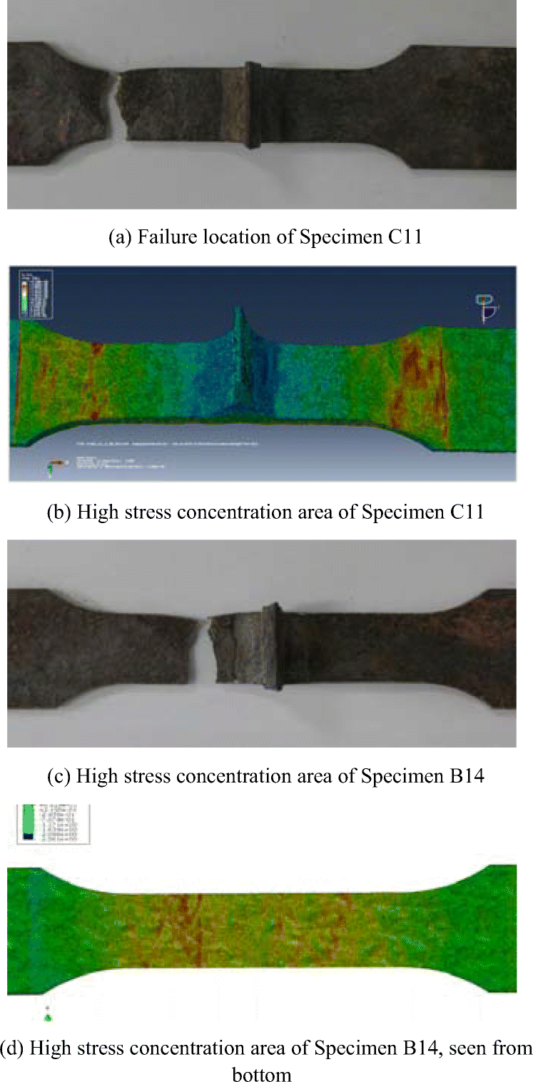Figure  10  Failure location and stress concentrations around specimen C11 and B14

Download: Full-Size Img

6   Conclusion

Analysis and comparative study of experimental and FE calculated SCFs of small-scaled corroded specimens was performed. The experimental SCFs are derived from experimentally estimated fatigue lives, by comparing it to the expected fatigue lives defined for perfectly smooth specimens. The SCFs were analysed by FEM using very fine 3D finite elements. The nodal plate thicknesses of FE models were identified by the photogrammetry method. A convergence study was performed to determine the element size and the accuracy of the estimated SCFs.

It was shown that the prediction of the experimental SCFs by the use of the FE analysis is unbiased, i.e. on an average, the calculated SCFs agree well with the experimental ones. However, the dispersion observed in the predictions is rather large, as measured by the standard deviation.

Linear regression trend lines, showing the dependency of SCFs on statistical properties of corroded surfaces, were generally better for calculated than for the experimentally estimated SCFs. It is interesting to notice that the trend lines presenting SCFs vs the mean value of the corroded specimen surface are almost identical for both SCF_FEM and SCF_Exp.

Similar SCFs are observed at several locations along with the specimen, making it difficult to predict precisely the failure location by FE analysis. However, in most of the cases analysed, one of the areas with the increased stresses identified from FE results coincides with the actual failure position obtained from experiments.