1   Introduction

Shipping is the most fuel-efficient means of moving freight, where more than 70% of global freight task is to transport by ships. Most of them are powered using diesel engines, which are considered the most fuel-efficient engines. They are installed in different types of ships ranging in size and application from small ships to large ocean-going vessels. These engines are operated using fuel either it is marine diesel oil (MDO) or heavy fuel oil (HFO), with a high level of sulfur for economical purposes. From 2000, strong restrictions are applied by the International Maritime Organization (IMO) and the International Convention for the Prevention of Pollution from Ships (MARPOL), to reduce the amount of sulfur oxides (SO_x) emissions from ships (IMO 2017) to reach its lowest level by 2020 as shown in Figure 1 for both emission control areas (ECAs) and non-ECAs as demonstrated in Figure 2. An International Air Pollution Prevention Certificate (IAPPC) must be issued for each ship according to Annex Ⅵ in MARPOL to ensure that all ships of 400 gross tonnage (GT) or above are committed with the requirements of Annex Ⅵ.

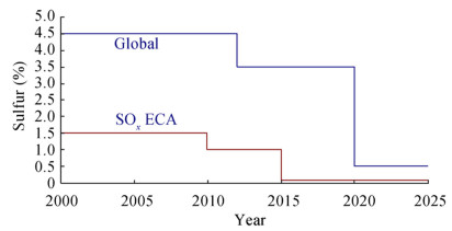Figure  1  MARPOL Annex Ⅵ SO_x emission limits (DieselNet 2017)

Download: Full-Size Img

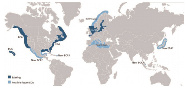Figure  2  Emission control areas (ECAs) around the world (Puisa 2015)

Download: Full-Size Img

Sulfur dioxide (SO₂) presents more than 95% of SO_x emissions emitted from the combustion of marine fuel. It is a colorless, bad-smelling, and toxic gas which has a direct effect on human health causing chest pain, eye irritation, and breathing problem at a lower level of concentration. It is a source of formation of sulfates and nitrates in the form of inorganic aerosols which are harmful to the human respiratory system. It can be fatal if it reaches 500 parts per billion (ppb) in the around atmosphere (EGCSA 2019). Also, SO₂ can be oxidized and converted into acids which are the main source of acid rain followed by many ecological effects (EPA 2019).

From that concept, different technologies are considered to control the amount of SO_x emissions from the marine industry.

Fossil fuel energy system must be improved for a better and cleaner future transportation for the world because it is responsible for 15% of the world nitrogen oxides (NO_x) and SO_x emissions (El-Gohary 2013). Based on the new regulations, the components of sulfur are reduced in the fuel to 1% in low sulfur diesel (LSD) and low sulfur fuel oil (LSFO), while the ultra-low sulfur diesel (ULSD) and ultra-low sulfur fuel oil (ULSFO) have been refined so that its sulfur content is less than or equal to 15 ppm. This is 97% cleaner than the standard fuel used (EPA 2017).

Currently, the sulfur limit in marine fuel is 0.1% in ECA and port areas and 3.5% in all other areas. Two strategies can be adapted to comply with these restrictions: the first, which is more expensive at the moment, is the installation of seawater scrubbers on board, reducing the SO_x content in exhaust emissions, and the second is the fuel switch from high sulfur residual fuel oil (HSRFO) to low sulfur distillate fuel oil (LSDFO) when crossing emission control areas. The first strategy is being widely adopted in new ships, while generally for existing ships the second is more convenient, at least until (presumably 2025) the limit will drop from 3.5% to 0.5%. The ships approaching the port areas are particularly relevant about the overall emissions (Iodice and Senatore 2015) for two reasons: First, the ship is in maneuvering mode, and the engine works at part load; moreover, the vessel is performing the fuel switch. Both these conditions alter the normal levels of engine emissions (Iodice et al. 2017).

Different alternative marine fuel types can be used in main and auxiliary engines to reduce the level of emissions due to the lack of sulfur component in these fuels (El-Gohary 2013; Banawan et al. 2010). They could be found in liquid form, including ethanol, methanol, bioliquid fuel, and biodiesel, and in gaseous form, including propane, hydrogen, and natural gas (NG). However, the different parts of the engines fueled with these alternative fuels must be optimized as in (Ambrós et al. 2015; Li et al. 2014; Karabektas 2009; Ng et al. 2013; Altosole et al. 2017) in order to reduce the exhaust emissions that are depending mainly on the amount of brake specific fuel consumption (BSFC). The BSFC can be defined as the measure for the fuel efficiency of any internal combustion engine; it is expressed in g/kW·h, which is the ratio between the rate of fuel consumption (expressed in g/s) and the brake power (expressed in kW). Obviously, lower values of this parameter are always required.

The hydrogen and the NG are receiving considerable attention in shipping due to their availability and their low cost, and they are free of carbon and sulfuric materials (El-Gohary 2012). El-Gohary and Seddiek (2013) presented the usage of both hydrogen and NG as alternative fuels to diesel oil for a marine gas turbine which lead to 100% reductions in SO_x emissions and particulate matter (PM) and 92% reduction in NO_x emissions and 25% reduction in carbon dioxide (CO₂) as compared with diesel fuel (Welaya et al. 2013b; El-Gohary et al. 2015). Hydrogen is also used to convert the chemical energy into electricity in the fuel cell technology (Welaya et al. 2011; Welaya et al. 2013a; Villalba-Herreros et al. 2017). However, it is very restricted due to some technical problems. The NG is used in the dual fuel engines that could be run also on HFO or MDO to verify the limitations of exhaust emissions applied by IMO (Wärtsilä 2017). The engine could smoothly switch from gas fuel to HFO/MDO operation and vice versa without loss of power or speed. The interaction between the gaseous fuel and the pilot fuel was considered in the study presented by Miao and Milton (2005). Stoumpos et al. (2018) simulated the performance of a marine dual fuel engine to reduce exhaust emissions and show a good reduction in BSFC and NO_x emissions. Also, Talekar et al. (2016) supported the dual fuel engine fueled with NG to improve the combustion efficiency and the reduction of exhaust emissions.

The biofuel becomes an alternative fuel for diesel engines despite its higher production cost than the MDO. It has been recognized and used by many countries around the world including the European Union (EU), the USA, Brazil and Asia (The Statistics Portal 2017). According to ETIP (2019), different types of biofuels are under investigation and expected to be widely used in the near future (Silitonga et al. 2013; Ong et al. 2014). One of the advantages of biodiesel is that the amount of different exhaust emissions can be reduced depending on the percentages of biodiesel-diesel blends than only using diesel oil such as carbon monoxide (CO), hydrocarbon (HC), PM, and SO₂ beside the CO₂ which are partially absorbed by the photosynthesis of plants (Silitonga et al. 2018; Mohd Noor et al. 2018; Clume et al. 2019).

Exhaust gas scrubber can be installed onboard instead of using marine fuels with low sulfur content in ECAs (Seddiek and Elgohary 2014), and it helps to reduce the SO_x emissions from ships by 98% (Ammar and Seddiek 2017). Scrubbers can be classified into two categories: dry and wet scrubber (ABS 2017). A dry scrubber does not use any liquid to carry out the scrubbing process; a chemical reaction between the hydrated lime-treated granulates and the exhaust gas removes the SO_x emissions compounds. In a wet scrubber, the exhaust gas passes through a liquid medium in order to remove the SO_x compounds from the gas by chemically reacting with parts of the wash liquid. The most common liquids are untreated seawater and chemically treated freshwater (MAN Diesel and Turbo 2014; Wärtsilä 2015). The main disadvantage in refitting a ship with this technology is the cost of several million euros, which leads to a loss in the income for the ship-owners (Jiang et al. 2014).

Good quality of lubricating oil with efficient control systems can control the amount of sulfur in the fuel and decrease SO_x emissions from the engine. Recently, pulse or alpha lubrication systems are the two control systems used. The tests showed that the exhaust emissions were reduced when the cylinder oil feed rate was also reduced. So the lubrication systems are optimized and controlled with a high-pressure electronically controlled lubricator that injects the cylinder lube oil into the cylinder at the exact position and time, which is not always possible with the conventional mechanical lubricators (MAN Diesel and Turbo 2016a).

Based on the mentioned technologies, different engine simulation models are developed to easily predict the performance of different types of engines for saving time and reducing the costs of doing experimental tests. However, by coupling one of the optimization methods (Hillier and Lieberman 1980) to these numeric codes depending on the faced problem, more accurate results can be achieved. From that concept, this study presents standard procedures, based on the experience of authors, to optimize the performance of any marine engine in order to minimize the fuel consumption and thus the exhaust emissions. Part of the results of these optimization procedures, along the engine load diagram, are presented in previous research papers by Tadros et al. (2018b) and Tadros et al. (2019).

An extension of the previous works in this paper discusses the computation of the formation of SO_x emissions after optimizing the performance of the two turbocharged four-stroke marine diesel engines fueled with MDO based on the amount of sulfur in the fuel to be further used in different numerical simulations. The results of this computation are important due to the unavailability of the value of SO_x emissions along the entire operating conditions of the two engines. The SO_x emissions are computed in g/kW·h and in ppm based on the optimized values of BSFC and air-fuel ratio (AFR) respectively for different operating conditions, by considering the percentage of sulfur in the fuel. Then a surrogate model-based response surface methodology (RSM) is applied to generate numerical equations using polynomial regression methods to present the variation of SO_x emissions for different engine speeds and loads. These non-dimensional equations can be integrated into further research to compute the amount of SO_x emissions for different percentages of sulfur of the selected or similar engines. Also, they can be integrated with different weather routing codes in order to present a technological and economic study of the fuel used and to compute the total amount of SO_x emissions from ships along their trips in both ECA and non-ECA areas.

2   Procedures for Optimum Engine Performance

In this section, an overview of the procedures required to optimize the performance of any marine diesel engine using 0D/1D is presented based on authors' experiences and some collected data from software manuals. Four procedures must be taken into consideration as shown in Figure 3:

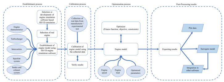Figure  3  General presentation for optimum engine performance

Download: Full-Size Img

1) Establishment process

2) Calibration process

3) Optimization process

4) Post-processing results

2.1   Establishment Process

This process is the first part to simulate the performance of any diesel engine using any 0D/1D model. It consists of the three steps as follows:

1) The first step is to develop the simulation code using any of the programming languages such as MATLAB/Simulink, Python, Visual Basic, LabVIEW, C, or C++ to select an available commercial engine simulation software such as Ricardo Wave, GT-suite, or AVL for model implementation.

2) The second step is to select a real engine and collect its data either from the project guide of the manufacturer or from experimental tests performed in the engine laboratory.

3) The final step in this process is the establishment of the engine model in the simulation software taking into account the different parts of the engine as shown in Figure 4, such as engine characteristics, turbocharger, intercoolers, injection system, and intake and exhaust systems. After that, it is required to define the properties of air and fuel used, the atmospheric initial conditions, and the initial pressure and temperature of each duct and junction. Finally, different sub-models must be selected or defined to compute the combustion, conduction, heat transfer, friction, and the amount of the different exhaust emissions.

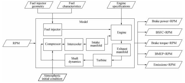Figure  4  Schematic diagram of the simulation model (Tadros et al. 2016)

Download: Full-Size Img

2.2   Calibration Process

After ensuring that the engine model is built correctly without any types of errors, in this section, generic procedures are presented to be used as guidelines to calibrate the model. First of all, the calibration process must be performed at high engine speed and high load in order to check that the engine model will be able to reach this high amount of power. By considering the volumetric efficiency and brake power or torque, the model can be smoothly calibrated. Then, the calibration will be performed for different engine speeds and loads.

2.2.1   Volumetric Efficiency

The volumetric efficiency is the best indicator to maximize the engine breathing or the mass flow rate inside the engine.

It assists in the selection and scaling of the maps of the turbocharger from existing ones if their data are not available.

Once this pre-run is finished, the volumetric efficiency, mass flow rate, plenum temperature, and plenum pressure must be compared against the measured data as the main checklist. This gives the opportunity to check and modify the valves' timing, the wall temperature and the heat transfer multiplier along the intercooler, and the intake and exhaust systems.

2.2.2   Brake Power or Torque

After calibrating the engine model based on the volumetric efficiency as described in the previous point, the calibration of the brake power or torque takes place to increase the accuracy of the simulated results. This part focuses on calibrating the combustion process where the amount of AFR is checked and compared against real data. This leads to choose and calibrate the combustion model by selecting the appropriate type of Wiebe function as presented in detail by Ghojel (2010). Also, it helps to verify the firing pressure inside the cylinder and then verify the exhaust pressure and temperature from the cylinders to ensure the safety of the engine.

2.3   Optimization Process

Once finalizing the calibration process, the engine model is connected to an optimizer either in the same software used or in any third-party software to easily control the values of the selected parameters for different engine speeds and loads. Sometimes, this process can be used to recalibrate the engine model to improve the accuracy of the computed results. In the optimization model, the boundary conditions of each parameter are defined; then the fitness function is constructed including the objective function of the study and the penalty function to express constraints. Different penalty functions can be evaluated (Yeniay 2005), while the authors recommend the use of the static penalty function as it shows a good agreement with the real data (Tadros et al. 2019), and it was considered in different previous engine studies (Zhao and Xu 2013; Zhu et al. 2015).

2.4   Post-Processing Results

After computing the performance of the engine along the load diagram, the results can be combined, visualized, and analyzed. For instance, different surrogate models or any machine learning method can be applied to the computed data to study the relationship between the different parameters. Also, this data can be integrated into any other software/codes for more practical research (Vettor and Guedes Soares 2016; Vettor et al. 2018; Zaccone et al. 2018; Tadros et al. 2018a).

3   Model Implementation

3.1   Establishment Process

By following the procedures described in the previous section, two marine diesel engines are selected to perform the simulation and the optimization procedures. The first engine chosen for simulation is the MAN R6-730. It is a marine turbocharged diesel engine, 4-stroke, 6 cylinder in-line, with a speed range of 1000–2300 r/min producing 537 kW (MAN Diesel and Turbo 2017). It is used to propel small vessels such as yachts and patrol boats. The second engine chosen is the large MAN 18V32/44CR. It is also a 4-stroke marine turbocharged diesel engine with 18 cylinder and 750 r/min rated speed delivering 9180 kW (MAN Diesel and Turbo 2016b). It is designed for the propulsion of large ships like tankers, bulk carriers, containers, and ferries. Both engines satisfy the level of exhaust gas of tier 2 as defined in IMO MARPOL Annex Ⅵ. Table 1 shows the main characteristics of the two engines, and Table 2 presents the uncertainty of engine performance and exhaust emissions parameters based on environmental factors, approximation methods used, and data collected from the manufacturer.

The two engines are built in Ricardo Wave Software (2016) by connecting the different parts of each engine through junctions and pipes. As presented above, the turbocharger, intercooler, injection system, intake and exhaust systems, and engine cylinders are defined according to the engine structure. The friction, heat transfer, combustion, and exhaust emissions modules are defined as well. The simulation of the engine is performed according to the energy and momentum equations presented in Watson and Janota (1982) based on the concept of "filling and emptying" method, and the processes inside each cylinder are calculated according to the first law of thermodynamics (Heywood 1988) taking into consideration the heat release rate (HRR) depending on the Wiebe function which controls the burned mass fraction. The Wiebe function used in this study is the one suggested by Watson et al. (1980) which shows a good ability to simulate the combustion process of a marine Genset (Tadros et al. 2020b), while the heat transfer inside the cylinders is calculated using the empirical formula suggested by Woschni (1967). The heat transfer inside the pipes in the intake and exhaust manifolds and in the intercooler are calculated using the Colburn analogy (Bergman et al. 2011).

Then, the main exhaust emissions from engines are computed. The CO₂ emissions are calculated as functions of the BSFC using the emission factor suggested by Kristensen (2012) as they depend on the amount of carbon in the fuel. The NO_x emissions are calculated using the extended Zeldovich mechanism taking into consideration the two zones of combustion (Heywood 1988).

Finally, the formation of SO_x emissions is computed and is presented in this study. They depend on the amount of sulfur inside the fuel. It is composed of SO₂ and small amounts of sulfur trioxide (SO₃). Due to the unavailability of the calculation of SO_x emissions in Ricardo Wave, they are computed as SO₂ and as functions of BSFC using the empirical formula in Eq. (1) suggested by Lloyd's Register (1995). The amount of SO_x emissions in g/kW·h is directly proportional to the BSFC; once the BSFC increases, the SO_x emissions increases and vice versa.

This is why the new technologies (Woodyard 2004) and artificial intelligence (Mohd Noor et al. 2015; Tadros et al. 2020a) must be used to minimize the fuel consumed for the same operating point.

Furthermore, they are computed in ppm based on the amount of AFR as in Eq. (2) suggested by Mao and Wan (2000). Besides the amount of sulfur in the fuel that is required to be reduced, an increase in the AFR can assist in the reduction of the formation of SO_x emissions for the same operating point. The AFR can be increased in several ways; the most effective one is using high performance turbocharger and variable valve timing (VVT) as in modern engines, to increase the engine volumetric efficiency (VE) and thus AFR.

where %S is the percentage of sulfur in fuel, $ {M}_{{{\rm{SO}}}_2} $ is SO₂ molar weight, and M_S is S molar weight.

3.2   Calibration Process

After the establishment of the two numerical engine models, the calibration procedures take place by taking into account the thermo-fluid properties along the different parts of the engine, and a good agreement is achieved between the calculated and read data as shown in (Tadros et al. 2019). Figures 5 and 6 show the difference between the calculated BSFC and the data provided from the manufacturer for MAN R6-730 at the theoretical propeller curve and at the full load respectively for different engine speeds and loads with an average error 1.11% and 2.73%, respectively, while Figure 7 shows a comparison between the numerical results and the real data of BSFC for MAN 18V32/44CR. A good fitting is achieved between the real and the numerical curves for each engine with a 1.6% average error along the different operating conditions.

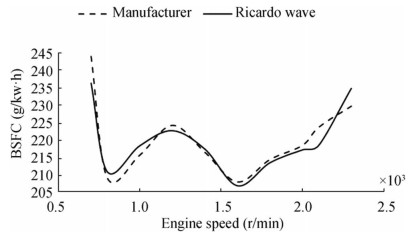Figure  5  Comparison between the values of BSFC at the theoretical propeller curve of the manufacturer and Ricardo Wave for MAN R6-730 (Tadros et al. 2018b)

Download: Full-Size Img

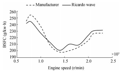Figure  6  Comparison between the values of BSFC at the maximum load of the manufacturer and Ricardo Wave for MAN R6-730 (Tadros et al. 2018b)

Download: Full-Size Img

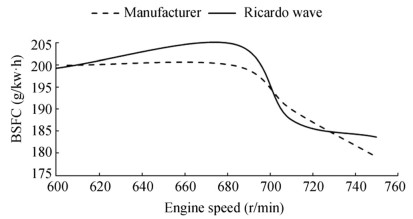Figure  7  Comparison between the values of BSFC at the theoretical propeller curve of the manufacturer and Ricardo Wave for MAN 18V32/44CR (Tadros et al. 2018b)

Download: Full-Size Img

3.3   Optimization Process

In order to increase the accuracy of the model and to easily estimate the optimum performance of the engine along the different engine speeds and loads, an optimization method is coupled to the engine model to easily predict the optimum values of the different input parameters instead of losing time doing manually. An engine optimization model was developed by Tadros et al. (2019) to find the optimum values of turbocharger speed (TS), the start of injection (SOI), the intake valve opening (IVO), and the amount of fuel rate (FR) along the different engine speeds and loads. The performance of the marine diesel engines is simulated by minimizing the BSFC, by verifying the NO_x emissions limitations applied by the IMO, and by verifying the firing pressure and the exhaust temperature inside the engine for safety aspects. The developed model coupled Ricardo Wave Software (2016) as 1D engine simulation software with a nonlinearly constrained optimizer based on the interior point algorithm as shown in Figure 8. This model shows a good simulation time to find the optimal values of the turbocharger, injection system, and valve timing in order to assess the objective of the study. The engine model was adapted for each type of engine due to its different configurations.

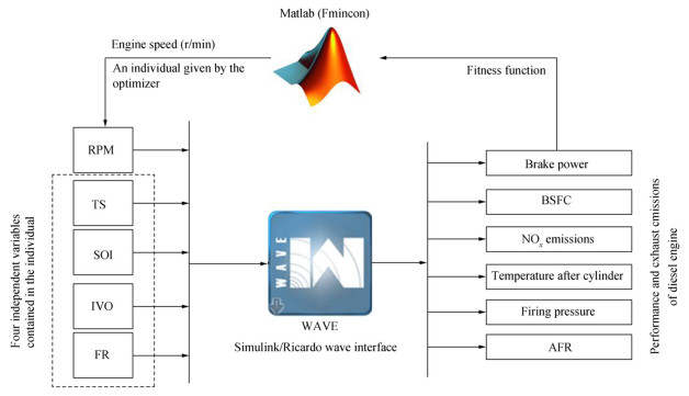Figure  8  Schematic diagram of engine optimization model (Tadros et al. 2019)

Download: Full-Size Img

4   Results and Discussion

4.1   Simulation of SO_x Emissions

After following the procedures presented above, the performance of each engine selected is calculated from the developed optimization model along the engine load diagram. The BSFC is minimized for the different operating conditions, and the engine model verifies the exhaust emissions and the safety aspects of the engines by optimizing the values of the parameters of the turbocharger, injection system, and valve timing. Figures 9, 10, 11 and 12 show the variation of BSFC and AFR for different engine speeds and loads for MAN R6-730 and MAN 18V32/44CR respectively. Some of these figures are collected from previous research papers for further clarification (Tadros et al. 2018b; Tadros et al. 2019).

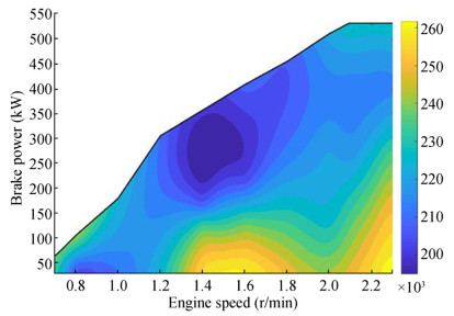Figure  9  Variation of BSFC in g/kW·h along the engine load diagram of MAN R6-730 (Tadros et al. 2018b)

Download: Full-Size Img

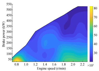Figure  10  Variation of AFR along the engine load diagram of MAN R6-730

Download: Full-Size Img

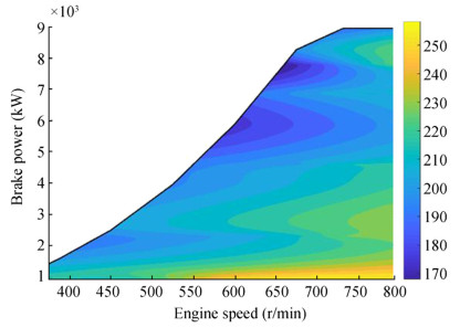Figure  11  Variation of BSFC in g/kW·h along the engine load diagram of MAN 18V32/44CR (Tadros et al. 2019)

Download: Full-Size Img

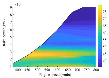Figure  12  Variation of AFR along the engine load diagram of MAN 18V32/44CR (Tadros et al. 2019)

Download: Full-Size Img

Once the BSFC and AFR are computed, SO_x emissions can be calculated based on the standard amount of sulfur (2.5%S) in diesel fuel or any other values according to the fuel used and compared with the real data measured from the manufacturer or from experimental tests. SO_x emissions can be computed in g/kW·h and in ppm using Eqs. (1) and (2) respectively according to the calculated BSFC and AFR.

Figures 13 and 14 show the variation of SO_x emissions in g/kW·h for MAN R6-730 and MAN 18V32/44CR respectively based on the standard amount of sulfur. The results are validated using data from the manufacturer at the rated speed, and it is noticed that SO_x emissions decrease in the high loads and vice versa as proportional to the BSFC values.

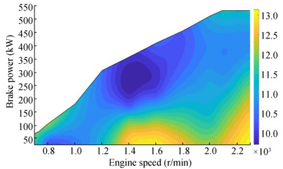Figure  13  Variation of SO_x emissions in g/kW·h of MAN R6-730 for 2.5%S

Download: Full-Size Img

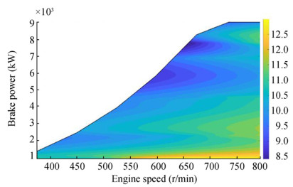Figure  14  Variation of SO_x emissions in g/kW·h of MAN 18V32/44CR for 2.5%S

Download: Full-Size Img

Figures 15 and 16 show the variation of SO_x emissions in ppm based on the AFR. Due to a large amount of fuel that is injected at the high loads, the formation of SO_x emissions increases, while a reduction in SO_x emissions is achieved at the low loads. These values of SO_x emissions either in g/kW·h or in ppm can be changed according to the amount of sulfur inside the fuel used. Also, it is important to mention for further investigations that the normal operating area of these engines will be from 85% to 100% of engine speed for both engines and from 60% to 90% of engine load for large engine and from 50% to 85% of engine load for the small one.

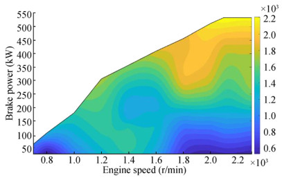Figure  15  Variation of SO_x emissions in ppm of MAN R6-730 for 2.5%S

Download: Full-Size Img

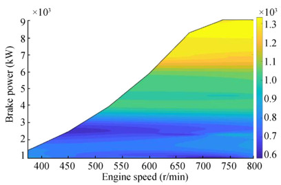Figure  16  Variation of SO_x emissions in ppm of MAN 18V32/44CR for 2.5%S

Download: Full-Size Img

4.2   Response Surface Methodology

The RSM is one of the methods used as a surrogate model suggested by Box and Wilson (1951) to generate a surface response using a polynomial model. This surface describes the relationship between the input and the output parameters. It is widely used to simplify a complex system such as a diesel engine. As an extension of the surrogate model presented by Tadros et al. (2018b), a fourth polynomial regression model in Eq. (3) is adopted fitting better the calculated data from numerical models than the lower-order model, where the equations of BSFC, CO₂, and NO_x emissions are generated for each engine, function of speed, and load.

where x is the engine speed and y is the brake power and both of them are non-dimensional.

In this study, the coefficients of equation of BSFC that are computed by Tadros et al. (2018b) will be considered to compute the formation of SO_x emissions using Eq. (1), while AFR surface is generated using the fourth polynomial regression model to be considered during the computation of SO_x emissions in ppm using Eq. (2). Engine speeds and loads are expressed as percentages from the rated speed and the rated power respectively. Also, the equations of BSFC and AFR are computed as a percentage of BSFC and AFR at the rated speed respectively. So these equations can be adapted to estimate the SO_x emissions for different levels of sulfur and for other similar engines with a different rated value of BSFC and AFR without performing again all the complicated simulations.

The curves of the load limit MAN R6-730 and MAN 18V32/44CR are presented in Eqs. (4) and (5) to define the limits of the brake power for each engine speed.

The generated surface of BSFC and AFR of MAN R6-730 show goodness of fitting with R-square equals to 0.8983 and 0.8718 respectively. The coefficients of the equations are presented in Table 3.

The generated surface of BSFC and AFR of MAN 18V32/44CR show goodness of fitting with R-square equals to 0.9340 and 0.9109 respectively. The coefficients of the equations are presented in Table 4.

5   Conclusion

In this study, different techniques for reducing the amount of SO_x emissions are discussed. A procedure is presented to establish, calibrate, and optimize the performance of any marine engine model to achieve minimum fuel consumption and exhaust emissions. Then an extension of previous computations is performed to estimate the amount of SO_x emissions along the engine load diagrams of two different marine diesel engines.

It has been concluded that the performance of the engine must be optimized to minimize the amount of formation of SO_x emissions as they depend on the value of the BSFC and the amount of AFR.

Based on the optimized results, response surface methodology is used to generate non-dimensional equations functions of speed and load for the BSFC and AFR to assess the amount of SO_x emissions in g/kW·h and in ppm, respectively, based on a given percentage of fuel sulfur for the considered or similar engines.

These non-dimensional equations can be further used to estimate the performance of the marine engines without preforming any detailed simulation and can be integrated into different marine applications.

This study opens the door to perform a technological and economic study of optimizing other types of engines powered by different types of fuel and various types of after-treatment systems along the trip of different ships.