-
Abstract
In this study, a series of numerical calculations are carried out in ANSYS Workbench based on the unidirectional fluid–solid coupling theory. Using the DTMB 4119 propeller as the research object, a numerical simulation is set up to analyze the open water performance of the propeller, and the equivalent stress distribution of the propeller acting in the flow field and the axial strain of the blade are analyzed. The results show that FLUENT calculations can provide accurate and reliable calculations of the hydrodynamic load for the propeller structure. The maximum equivalent stress was observed in the blade near the hub, and the tip position of the blade had the largest stress. With the increase in speed, the stress and deformation showed a decreasing trend.-
Keywords:
- Marine propeller ·
- Stress distribution ·
- Deformation distribution ·
- Open water performance ·
- Fluid ·
- solid coupling
Article HighlightsAn increase in the power of the host increases the load per unit area of the propeller, which requires a high strength of the propeller.The stress distribution and blade deformation of the propellers made of different materials at different forward speeds have been obtained using the FSI technique.Open Access This article is licensed under a Creative Commons Attribution 4.0 International License, which permits use, sharing, adaptation, distribution and reproduction in any medium or format, as long as you give appropriate credit to the original author(s) and the source, provide a link to the Creative Commons licence, and indicate if changes were made. The images or other third party material in this article are included in the article's Creative Commons licence, unless indicated otherwise in a credit line to the material. If material is not included in the article's Creative Commons licence and your intended use is not permitted by statutory regulation or exceeds the permitted use, you will need to obtain permission directly from the copyright holder. To view a copy of this licence, visit http://creativecommons.org/licenses/by/4.0/.A numerical simulation is set up to analyze the open water performance of a propeller.The stress and deformation distribution under different working conditions and their relationship with material have been analyzed. -
1 Introduction
With the development of large-scale civil ships, the unevenness of the wake flow field at the surface of the ship's propeller has increased, causing deterioration in the working environment of the propeller. An increase in the power of the host increases the load per unit area of the propeller. These effects require a high strength of the propeller. To improve the propeller strength, the minimum thickness of the propeller blade and the stress distribution of the blade must be considered (Zhao 2003). Many scholars have conducted research on the hydrodynamic performance of propellers and developed many research methods, such as the lifting-line method (Lerbs 1952), lifting-surface method (Sparenberg 1960; Tsakonas et al. 1966; Cummings 1973; Kerwin and Lee 1978; Greeley and Kerwin 1982; Lee 1980), and panel method (Kerwin 1987; Lee 1987; Yamasaki and Ikehata 1992; Koyama 1994; Hoshino 1990). Several scholars have also examined the strength of propellers using fluid–structure interaction (FSI) methods. Lin and Lin (1996) used the lift-surface method and nine-node degenerated shell finite element coupling algorithm to understand the hydrodynamic performance of propellers made of composite materials. Young (2007) studied the panel method and method coupled ABAQUS with the propeller hydroelastic calculation. Zhang et al. (2014) examined the influence of the deformation of propeller blades on the surface pressure, surrounding flow field, and open water performance by using the FSI method. Yang et al. (2015) used computational fluid dynamics (CFD) based on the viscous flow theory combined with the finite element software to calculate the bidirectional FSI of glass fiber composite propellers and nickel–aluminum bronze propellers without considering the laminate structure. He et al. (2014) conducted a numerical simulation of the FSI of a propeller based on the Visual Basic for Applications (VBA) technology in a general-use software, MS Excel, combined with a self-developed propeller hydrodynamic analysis code and a secondary development of a structural commercial software. Zou et al. (2017) discussed the influence of a hub on the performance of a propeller under FSI. Huang et al. (2015) compared the accuracy of calculations of a propeller made of the same metal material using the FSI method and the traditional CFD method. Ren et al. (2015) used the unidirectional FSI and bidirectional FSI methods to calculate and compare the static stress and total deformation of a propeller. Wang et al. (2014) used the unidirectional FSI method to calculate and analyze the structural strength of the propeller and verified the rationality of the method by comparing it with the safety factor recommended in the literature. Huang et al. (2017a, 2017b, 2017c) conducted many studies on composite propellers, compared them with copper propellers, and found that composite propellers are more susceptible to hydrodynamic loads. Li et al. (2018) analyzed the added mass and damping matrices due to FSI and examined the effects of the propeller's skew angle and incoming flow velocity on the two matrices. Li et al. (2019) calculated the hydrodynamic performance and structural response of a composite DTMB 4381 propeller in a heterogeneous flow field in ANSYS Composite PrepPost (ACP).
In this study, we verify the reliability of the hydrodynamic load calculation by using CFD and use the ANSYS FLUENT unidirectional FSI method to calculate, analyze, and compare the equivalent stress and total deformation of a propeller at different advance speeds and study the propeller deformation characteristics of different materials.
When marine propellers are working, they are subject to multiple forces, such as gravity, centrifugal force, and hydrodynamic load. The stress is complex, which leads to cavitation erosion, fatigue fracture, and other problems. Previous studies have validated the feasibility of FSI in the analysis of propeller strength. In this study, the numerical simulation is extended to off-design conditions. Moreover, a composite propeller has become increasingly popular in engineering applications. Both of these problems deserve more detailed investigations. Here, a numerical calculation of propeller hydrodynamics is performed and compared with experimental data in the literature. Then, the hydrodynamic force is applied to the propeller through the finite element method, and the size and distribution of the equivalent force and axial strain of propellers made of different materials in open water are determined, which can provide a theoretical basis for the design optimization of propellers.
2 Theoretical Basis
2.1 Hydrodynamic Analysis
The propeller rotating in a viscous fluid at a certain speed is simulated.
The continuity equation can be expressed as
$$ \frac{\partial \rho }{\partial t}+\frac{\partial }{\partial {x}_i}\left(\rho {u}_i\right)=0 $$ (1) where ρ is the liquid density and ui is the velocity.
The momentum equation can be expressed as
$$ \frac{\partial }{\partial t}\left(\rho {u}_i\right)+\frac{\partial }{\partial {x}_j}\left(\rho {u}_i{u}_j\right)=-\frac{\partial p}{\partial {x}_i}+\frac{\partial }{\partial {x}_j}\left(\mu \frac{\partial {u}_i}{\partial {x}_j}-\rho \overline{{u_i}^{\hbox{'}}{u_j}^{\hbox{'}}}\right)+{S}_i $$ (2) where p is the static pressure, measured in Pa; μ is the turbulent viscosity; ρ is the liquid density, measured in kg/m3; −ρui'uj' is the Reynolds stress term, measured in Pa; and S is the source term.
The k-ε Shear Stress Transfer (SST) turbulence model adopted in this paper has the following equations:
$$ {\displaystyle \begin{array}{l}\rho \frac{D k}{D t}=\frac{\partial }{\partial {x}_i}\left[\left(\mu +\frac{\mu_t}{\sigma_k}\right)\frac{\partial k}{\partial {x}_i}\right]+{G}_k+{G}_b-\rho \varepsilon -{Y}_M\\ {}\rho \frac{D\varepsilon}{D t}=\frac{\partial }{\partial {x}_i}\left[\left(\mu +\frac{\mu_t}{\sigma_k}\right)\frac{\partial \varepsilon }{\partial {x}_i}\right]+{C}_1\frac{\varepsilon }{k}\left({G}_k+{C}_3{G}_b\right)-{C}_2\rho \frac{\varepsilon^2}{k}\end{array}} $$ (3) where k is the turbulent kinetic energy; ε is the turbulent dissipation rate; Gk is the turbulent kinetic energy caused by the change in the average velocity gradient of a fluid particle; Gb is the turbulent kinetic energy caused by buoyancy; YM represents the effect of the turbulent fluctuating expansion on the total dissipation rate; μt is the turbulence viscosity coefficient; and C1, C2, and C3 are the constant coefficients.
The velocity inlet boundary condition can be described as
$$ {\displaystyle \begin{array}{l}\left(u,v,w\right)={\left(u,v,w\right)}_{\mathrm{given}}\\ {}\frac{\partial p}{\partial n}=0\end{array}} $$ (4) where u, v, and w are the velocity components.
The results show that the inlet velocity is given and the normal gradient of pressure is zero.
2.2 Structural Analysis
In this paper, the uniaxial FSI method is used to calculate the force applied on the propeller at a steady state. The finite element equation of the static analysis is as follows:
$$ \boldsymbol{Ku}=\boldsymbol{F} $$ (5) where K is the stiffness matrix of the propeller; u is the displacement vector matrix of the propeller node; and F is the load applied on the propeller, consisting of centrifugal force, gravity, and fluid pressure.
3 Numerical Simulation of the Flow Field
In the third part, the numerical calculation of the propeller hydrodynamics is performed and compared with the experimental data in the literature. Then, the hydrodynamic force is applied to the propeller by using the finite element method to complete the strength calculation and analysis.
3.1 Propeller Parameters
The DTMB P4119 propeller used in this study is a three-bladed propeller without side slant and back tilt. Its dimensions are listed in Table 1 (Yin and Kinnas 2001).
Table 1 Geometric features of the propellerDiameter (m) Number of blades Pitch ratio (0.7r) Hub diameter ratio Vertical tilt angle (°) Side tilt angle (°) Blade section 0.3048 3 1.084 0.2 0 0 NACA660mod 3.2 CFD Calculation Model
The entire computational domain is divided into two parts: rotational domain and static domain. The diameter of the static field is 4D, the entrance boundary diameter is 2.5D from the propeller, and the exit boundary diameter is approximately 3.5D from the propeller. The rotating cylindrical domain has a diameter of 1.2D and a length of 0.7D. The rotating and stationary domains use a high-quality hexahedral structured mesh and transfer the data by defining an interface with a total of 2.5 million meshes. The turbulence model uses the SST model. The propeller flow field computational domain is shown in Figure 1.
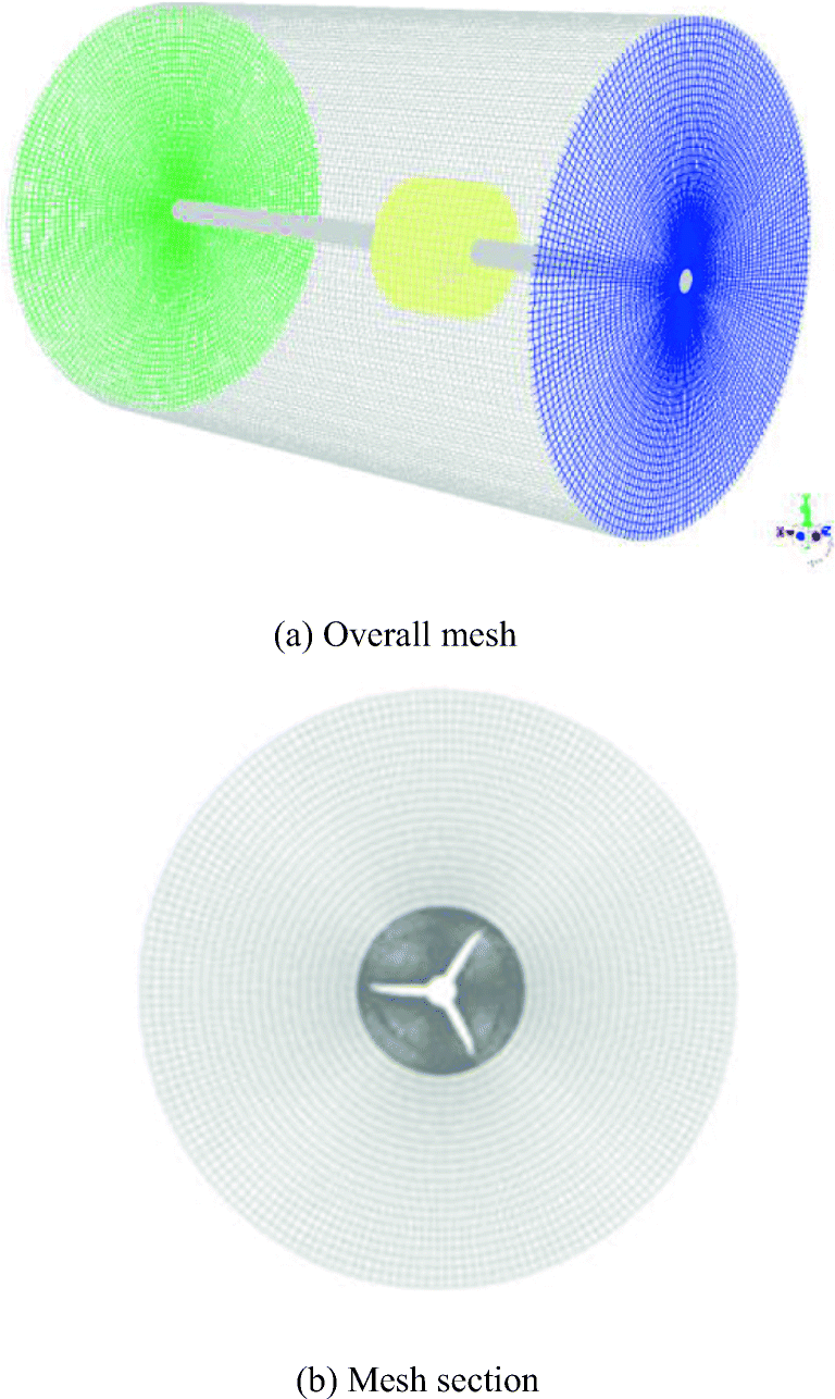 Figure 1 Computational domain of the propeller flow field
3.3 Boundary Condition Setting
The static domain is stationary relative to the absolute coordinate system, and the rotation domain is rotating at a constant velocity around the x-axis with a magnitude of –600 r/min with respect to a set dynamic reference system. The inlet is set as the speed inlet, given the inflow velocity at the corresponding speed coefficient; the outlet is set as the outflow boundary; and the blade and hub wall are set to no-slip solid wall.
The calculation relationship between the forward speed and the forward speed coefficient is
$$ J=\frac{V_A}{nD} $$ (6) where n is the propeller rotational speed, D is the diameter of the propeller, and VA is the flow speed at the inlet.
3.4 Calculation Results
3.4.1 Calculation of Open Water Performance
The solution formula for the hydrodynamic coefficient is as follows:
$$ {K}_T=\frac{T}{\rho {n}^2{D}^4};{K}_Q=\frac{Q}{\rho {n}^2{D}^5};\eta =\frac{J}{2\pi}\cdot \frac{K_T}{K_Q} $$ (7) where KT is the thrust coefficient, T is the thrust force, KQ is the torque coefficient, Q is the torque, η is the efficiency, and J is the forward speed coefficient.
The forward speed coefficient has values of 0.4, 0.5, 0.6, 0.7, 0.8, 0.833, 0.9, 1.0, and 1.1. The comparison results of the test value under the specific speed coefficient are shown in Table 2 (Miao and Sun 2011).
Table 2 Calculation results of open water performanceJ Calculated value Test value KT 10KQ η KTe 10KQe ηe 0.5 0.285 0.475 0.477 0.285 0.477 0.475 0.7 0.194 0.353 0.612 0.200 0.360 0.619 0.833 0.134 0.272 0.654 0.146 0.280 0.691 0.9 0.104 0.230 0.649 0.120 0.239 0.719 1.1 0.012 0.091 0.227 0.034 0.106 0.562 Based on these results, a graph is drawn, as shown in Figure 2.
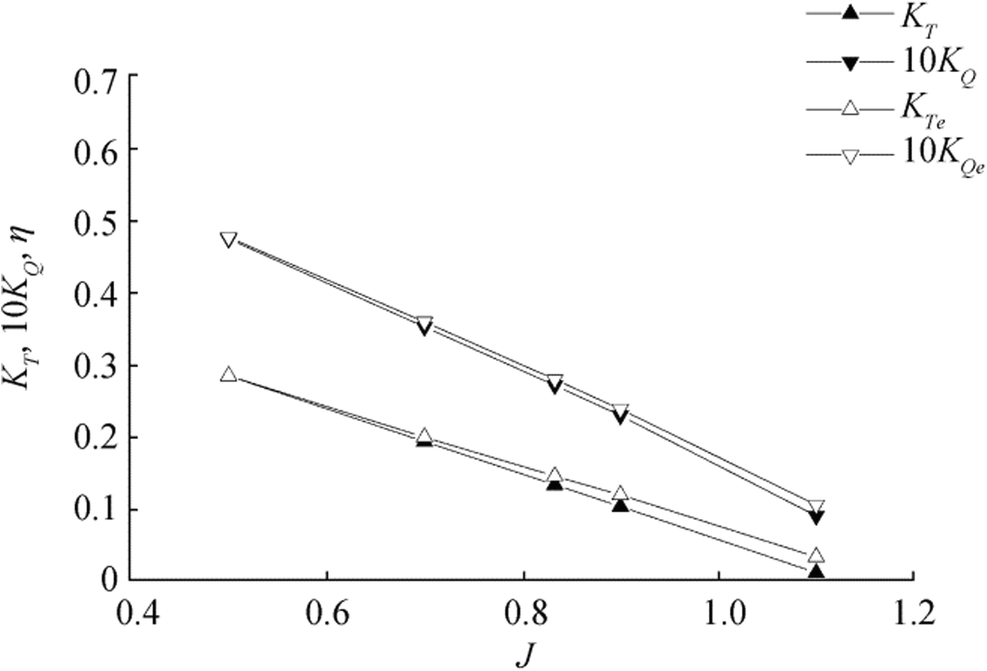 Figure 2 Comparison of the calculated and experimental results
It can be seen from Figure 2 that the numerical calculation results are similar to the literature test results, indicating that a reliable hydrodynamic load can be obtained from the numerical calculation.
3.4.2 Pressure Distribution on the Surface of the Blade
Taking the forward speed coefficients of 0.5, 0.833, and 1.1 as an example, the pressure distribution of the pressure surface and the suction surface of the blade is given, as shown in Figure 3.
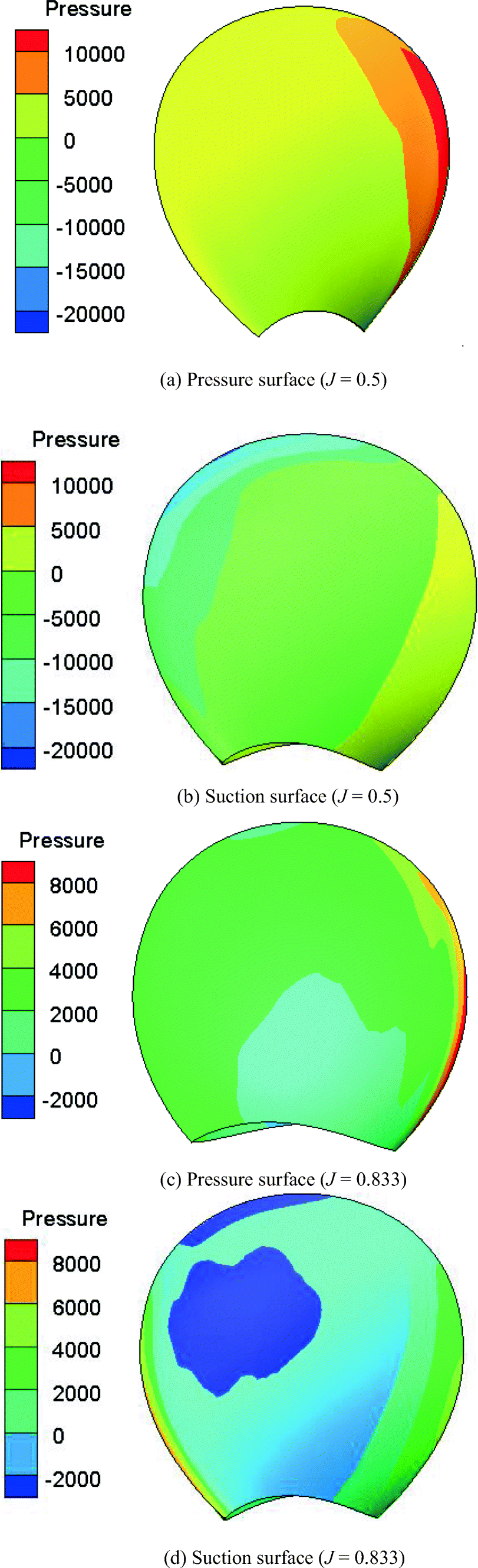 Figure 3 Pressure distribution of the blade surface
Figure 3 shows that the maximum pressure occurs at the leading edge of the propeller.
4 Finite Element Calculation of the Blade Stress
4.1 Propeller Meshing and Condition Setting
The propeller stress was calculated using the ANSYS WORKBENCH software. The finite element model is shown in Figure 4, and the number of meshes is 66 446. The propeller rotates around the x-axis at a fixed velocity of –600 r/min, applying a fixed-end boundary condition to both ends of the hub, and the hydrodynamic load is calculated by using FLUENT onto the finite element model of the propeller.
 Figure 4 FEA model of the propeller
The blade materials were selected from six different isotropic materials, as shown in Table 3.
Table 3 Propeller material characteristicsMaterial Density Young's modulus Poisson's ratio Alloy steel 7850 2E + 11 0.3 Nickel–aluminum bronze 7400 1.24E + 11 0.33 Copper alloy 8300 1.1E + 11 0.34 Titanium alloy 4620 9.6E + 10 0.36 Glass fiber 2100 2E + 10 0.18 Resin fiber 1800 3.53E + 09 0.14 4.2 Calculation Results
4.2.1 Stresses of Propellers Made of Different Materials
Table 4 shows the maximum equivalent stress and maximum deformation value of the blades for the six different isotropic materials at different speed factors. According to the values in Table 4, the curve of the maximum stress and maximum deformation with the advance speed coefficient is shown in Figures 5 and 6.
Table 4 Maximum stress and strain of propellers made of different materialsMaterials J 0.4 0.5 0.6 0.7 0.8 0.833 0.9 1.0 1.1 Alloy steel Stress/Pa 2.17E + 6 1.89E + 6 1.63E + 6 1.39E + 6 1.16E + 6 1.08E + 6 9.27E + 5 7.04E + 5 5.82E + 5 Deformation/m 1.22E − 5 1.00E − 5 8.23E − 6 6.64E − 6 5.22E − 6 4.78E − 6 3.95E − 6 2.88E − 6 1.95E − 6 Nickel–aluminum bronze Stress/Pa 2.17E + 6 1.88E + 6 1.62E + 6 1.38E + 6 1.15E + 6 1.07E + 6 9.17E + 5 6.93E + 5 5.76E + 5 Deformation/m 1.93E − 5 1.59E − 5 1.31E − 5 1.06E − 5 8.29E − 6 7.60E − 6 6.28E − 6 4.59E − 6 3.12E − 6 Copper alloy Stress/Pa 2.20E + 6 1.91E + 6 1.65E + 6 1.41E + 6 1.17E + 6 1.10E + 6 9.43E + 5 7.19E + 5 6.09E + 5 Deformation/m 2.18E − 5 1.80E − 5 1.47E − 5 1.19E − 5 9.37E − 6 8.59E − 6 7.11E − 6 5.22E − 6 3.56E − 6 Titanium alloy Stress/Pa 2.10E + 6 1.81E + 6 1.55E + 6 1.31E + 6 1.07E + 6 9.96E + 5 8.42E + 5 6.17E + 5 4.94E + 5 Deformation/m 2.44E − 5 2.01E − 5 1.64E − 5 1.32E − 5 1.04E − 5 9.49E − 6 7.82E − 6 5.71E − 6 3.88E − 6 Glass fiber Stress /Pa 2.00E + 6 1.72E + 6 1.46E + 6 1.22E + 6 9.91E + 5 9.16E + 5 7.64E + 5 5.44E + 5 3.69E + 5 Deformation/m 1.25E − 4 1.03E − 4 8.37E − 5 6.71E − 5 5.21E − 5 4.76E − 5 3.88E − 5 2.76E − 5 1.78E − 5 Resin fiber Stress/Pa 2.00E + 6 1.71E + 6 1.46E + 6 1.22E + 6 9.86E + 5 9.10E + 5 7.58E + 5 5.38E + 5 3.51E + 5 Deformation/m 7.14E − 4 5.87E − 4 4.78E − 4 3.83E − 4 2.98E − 4 2.71E − 4 2.21E − 4 1.56E − 4 9.98E − 5 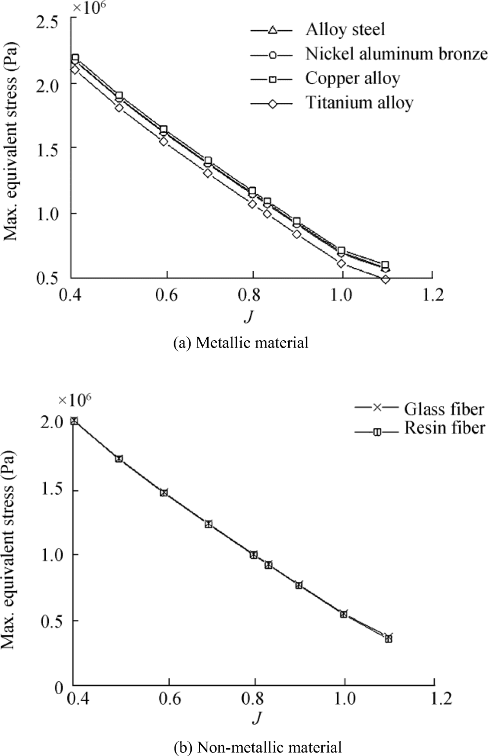 Figure 5 Maximum stress curve of the propellers made of different materials
 Figure 6 Maximum deformation curve of the propellers made of different materials
The analyses of Table 4, Figure 5, and Figure 6 show that with an increase in the forward speed coefficient, the maximum equivalent stress and the maximum deformation of propellers made of different materials decrease; the maximum deformation of the metallic propeller given in this study is higher by one magnitude compared with the maximum deformation of the non-metallic propeller; the deformation of the metallic propeller is very small and will have little influence on the flow field, indicating that it is reasonable to calculate the strength of the metallic propeller using the unidirectional FSI method.
4.2.2 Stress Distribution of the Propeller
Taking the nickel–aluminum bronze propeller as an example, the forward speed coefficients have values of 0.5, 0.833, and 1.1, and the equivalent stress and strain distribution of the propeller are analyzed, as shown in Figures 6, 7, and 8. The strain at the tip of the blade is the largest and gradually decreases toward the root of the blade; the equivalent stress in the middle of the blade root is the largest and decreases as it moves toward the tip of the blade.
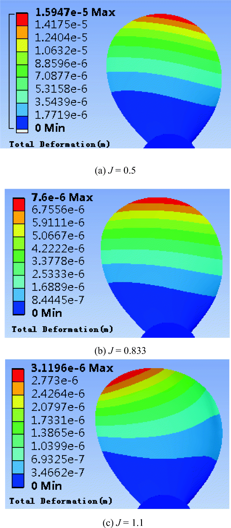 Figure 7 Deformation distribution of the propeller
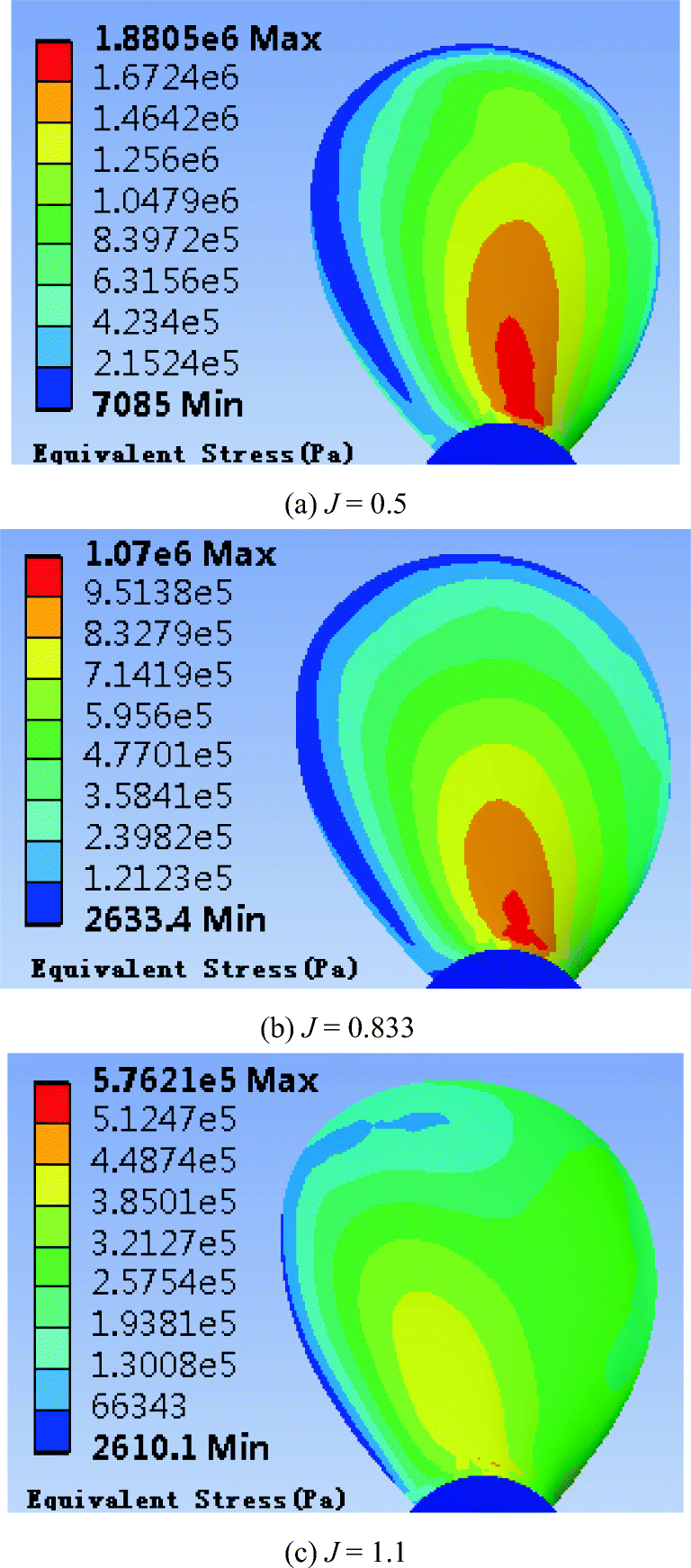 Figure 8 Stress distribution of the propeller
5 Conclusions
The hydrodynamic load on the propeller was calculated by using the CFD method, then the strength calculation on the blades of different materials was calculated, the stress and deformation distribution having been analyzed.
1) A numerical simulation is set up to analyze the open water performance of the DTMB 4119 standard propeller, and the simulation results are compared with test results from the literature to prove the reliability of the CFD calculation method.
2) Using ANSYS to perform a static analysis on the propeller, the stress distribution and blade deformation of the propellers made of different materials at different forward speeds can be obtained using the FSI technique.
3) In the future, more strength-sensitive propellers, such as highly skewed propellers, should be calculated.
-
Figure 1 Computational domain of the propeller flow field
Figure 2 Comparison of the calculated and experimental results
Figure 3 Pressure distribution of the blade surface
Figure 4 FEA model of the propeller
Figure 5 Maximum stress curve of the propellers made of different materials
Figure 6 Maximum deformation curve of the propellers made of different materials
Figure 7 Deformation distribution of the propeller
Figure 8 Stress distribution of the propeller
Table 1 Geometric features of the propeller
Diameter (m) Number of blades Pitch ratio (0.7r) Hub diameter ratio Vertical tilt angle (°) Side tilt angle (°) Blade section 0.3048 3 1.084 0.2 0 0 NACA660mod Table 2 Calculation results of open water performance
J Calculated value Test value KT 10KQ η KTe 10KQe ηe 0.5 0.285 0.475 0.477 0.285 0.477 0.475 0.7 0.194 0.353 0.612 0.200 0.360 0.619 0.833 0.134 0.272 0.654 0.146 0.280 0.691 0.9 0.104 0.230 0.649 0.120 0.239 0.719 1.1 0.012 0.091 0.227 0.034 0.106 0.562 Table 3 Propeller material characteristics
Material Density Young's modulus Poisson's ratio Alloy steel 7850 2E + 11 0.3 Nickel–aluminum bronze 7400 1.24E + 11 0.33 Copper alloy 8300 1.1E + 11 0.34 Titanium alloy 4620 9.6E + 10 0.36 Glass fiber 2100 2E + 10 0.18 Resin fiber 1800 3.53E + 09 0.14 Table 4 Maximum stress and strain of propellers made of different materials
Materials J 0.4 0.5 0.6 0.7 0.8 0.833 0.9 1.0 1.1 Alloy steel Stress/Pa 2.17E + 6 1.89E + 6 1.63E + 6 1.39E + 6 1.16E + 6 1.08E + 6 9.27E + 5 7.04E + 5 5.82E + 5 Deformation/m 1.22E − 5 1.00E − 5 8.23E − 6 6.64E − 6 5.22E − 6 4.78E − 6 3.95E − 6 2.88E − 6 1.95E − 6 Nickel–aluminum bronze Stress/Pa 2.17E + 6 1.88E + 6 1.62E + 6 1.38E + 6 1.15E + 6 1.07E + 6 9.17E + 5 6.93E + 5 5.76E + 5 Deformation/m 1.93E − 5 1.59E − 5 1.31E − 5 1.06E − 5 8.29E − 6 7.60E − 6 6.28E − 6 4.59E − 6 3.12E − 6 Copper alloy Stress/Pa 2.20E + 6 1.91E + 6 1.65E + 6 1.41E + 6 1.17E + 6 1.10E + 6 9.43E + 5 7.19E + 5 6.09E + 5 Deformation/m 2.18E − 5 1.80E − 5 1.47E − 5 1.19E − 5 9.37E − 6 8.59E − 6 7.11E − 6 5.22E − 6 3.56E − 6 Titanium alloy Stress/Pa 2.10E + 6 1.81E + 6 1.55E + 6 1.31E + 6 1.07E + 6 9.96E + 5 8.42E + 5 6.17E + 5 4.94E + 5 Deformation/m 2.44E − 5 2.01E − 5 1.64E − 5 1.32E − 5 1.04E − 5 9.49E − 6 7.82E − 6 5.71E − 6 3.88E − 6 Glass fiber Stress /Pa 2.00E + 6 1.72E + 6 1.46E + 6 1.22E + 6 9.91E + 5 9.16E + 5 7.64E + 5 5.44E + 5 3.69E + 5 Deformation/m 1.25E − 4 1.03E − 4 8.37E − 5 6.71E − 5 5.21E − 5 4.76E − 5 3.88E − 5 2.76E − 5 1.78E − 5 Resin fiber Stress/Pa 2.00E + 6 1.71E + 6 1.46E + 6 1.22E + 6 9.86E + 5 9.10E + 5 7.58E + 5 5.38E + 5 3.51E + 5 Deformation/m 7.14E − 4 5.87E − 4 4.78E − 4 3.83E − 4 2.98E − 4 2.71E − 4 2.21E − 4 1.56E − 4 9.98E − 5 -
Cummings DE (1973) Numerical prediction of propeller characteristics. J Ship Res 17(1): 12–18 https://doi.org/10.5957/jsr.1973.17.1.12 Greeley DS, Kerwin JE (1982) Numerical methods for propeller design and analysis in steady flow. Transactions - Soc Naval Arch Mar Eng 90: 415–453 He W, Tingqiu L, Ziru L (2014) Numerical simulation of fluid-solid coupling of propeller based on VBA. J Wuhan Univ Technol (Transmission Science and Engineering) 38(6): 1272–1276. https://doi.org/10.3963/j.issn.2095-3844.2014.06.020 Hoshino T (1990) Hydrodynamic analysis of propellers in steady flow using a surface panel method. Naval Arch Ocean Eng 28: 19–37. https://doi.org/10.2534/jjasnaoe1968.1989.55 Huang S, Bai XF, Sun XJ (2015) Numerical simulation of hydrodynamic performance of propeller based on fluid-solid coupling. Ships 1: 25–30. https://doi.org/10.3969/j.issn.1001-9855.2015.01.006 Huang Z, Xiong Y, Sun HT (2017a) Thicken and pre-deformed design of composite marine propellers. J Propulsion Technol 38(9): 2107–2114. https://doi.org/10.13675/j.cnki.tjjs.2017.09.024 Huang Z, Xiong Y, Yang G (2017) A fluid-structure coupling method for composite propellers based on ANSYS ACP module. Chin J Comput Mech 34(4): 501–506. https://doi.org/10.7495/j.issn.1009-3486.2017.04.006 Huang Z, Xiong Y, Yang G (2017) A comparative study of one-way and two way fluid-structure coupling of copper and carbon fiber propeller. J Nav Univ Eng 29(4): 31–35. https://doi.org/10.7511/jslx201704016 Kerwin J (1987) A surface panel method for the hydrodynamic analysis of ducted propellers. Soc Naval Arch Mar Eng-Trans 95: 93–122 Kerwin JE, Lee CS (1978) Prediction of steady and unsteady marine propeller performance by numerical lifting-surface theory. Sname Transactions 86: 1–30 Koyama K (1994) Application of a panel method to the unsteady hydrodynamic analysis of marine propellers. Unsteady Flow. Lee CS (1980) Prediction of the transient cavitation on marine propellers by numerical lifting-surface theory. Thirteenth Symposium on Naval Hydrodynamics, Tokyo Lee JA (1987) A potential based panel method for the analysis of marine propellers in steady flow. PhD thesis Department of Ocean Engineering Mit: 1987 DOI: 1721.1/14641 Lerbs HW (1952) Moderately loaded propellers with a finite number of blades and an arbitrary distribution of circulations. Transactions - Soc Naval Arch Mar Eng 60: 73–123 Li J, Zhang ZG, Hua H (2018) Hydro-elastic analysis for dynamic characteristics of marine propellers using finite element method and panel method. J Vib Shock 37: 22–29. https://doi.org/10.13465/j.cnki.jvs.2018.21.003 Li Z, Li G, He P, He W (2019) Numerical analysis of unsteady fluid-structure interaction of composite marine propellers. Huazhong Univ. of Sci. & Tech. 47(9): 7–13. https://doi.org/10.13245/j.hust.190902 Lin HJ, Lin J (1996) Nonlinear hydroelastic behavior of propellers using a finite-element method and lifting surface theory. J Mar Sci Technol 1(2): 114–124. https://doi.org/10.1007/BF02391167 Miao YY, Sun JL (2011) CFD Analysis of Hydrodynamic Performance of Propeller in Open Water. Chin Ship Res 6(5): 63–68. https://doi.org/10.3969/j.issn.1673-3185.2011.05.013 Ren H, Li F, Ling D (2015) Numerical calculation of influence of fluid-solid coupling on propeller strength. Journal of Wuhan University of Technology. Transp Sci Eng 39(1): 144–147. https://doi.org/10.3963/j.issn.2095-3844.2015.01.033 Sparenberg JA (1960) Application of lifting surface theory to ship screws. Int Shipbuild Prog 7(67): 99–106. https://doi.org/10.3233/ISP-1960-76701 Tsakonas S, Jacobs WR, Rank PHJ (1966) Unsteady propeller lifting-surface theory with finite number of chordwise modes. 12(1): 14-45. Wang H, Zhiwei Z, Zhibo Z (2014) Method for checking the strength of controllable-pitch propeller blade based on numerical calculation. Chin Ship Res 9(5): 53–59. https://doi.org/10.3969/j.issn.1673-3185.2014.05.010 Yamasaki H, Ikehata M (1992) Numerical analysis of steady open characteristics of marine propeller by surface vortex lattice method. J Soc Naval Arch Jpn 1992(172): 203–212. https://doi.org/10.2534/jjasnaoe1968.1992.172_203 Yang G, Ying X, Zheng H (2015) Two-way fluid-solid coupling calculation of composite propeller. Ship Sci Technol 37(10): 16–20. https://doi.org/10.3404/j.issn.1672-7649.2015.10.004 Yin LY, Kinnas SA (2001) A BEM for the prediction of unsteady midchord face and/or back propeller cavitation. J Fluids Eng 123(2): 403–419. https://doi.org/10.1115/1.1363611 Young YL (2007) Time-dependent hydroelastic analysis of cavitating propulsors. J Fluids Struct 23(2): 269–295. https://doi.org/10.1016/j.jfluidstructs.2006.09.003 Zhang S, Zhu X, Zhenlong Z, Hailiang H (2014) Analysis of fluid-solid coupling characteristics of propellers of the easily deformable ships. J Nav Univ Eng 1:48–53. https://doi.org/10.7495/j.issn.1009-3486.2014.01.011 Zhao B (2003) Research on the strength of large-slanting propeller. Huazhong Univ Sci Technol. https://doi.org/10.7666/d.y498868 Zou J, Jie X, Hanbing S, Zhen R (2017) Study on the influence of hub shape on propeller performance considering fluid-solid coupling. Ship 28(1): 21–28. https://doi.org/10.19423/j.cnki.31-1561/u.2017.01.021
| Citation: |
Kai Yu, Peikai Yan, Jian Hu (2020). Numerical Analysis of Blade Stress of Marine Propellers. Journal of Marine Science and Application, 19(3): 436-443. https://doi.org/10.1007/s11804-020-00161-3

|