1   Introduction

Planing hull forms in principle attain dynamic lift beyond a threshold speed. The same light hull which performs well at the pre-planing transition speed may exhibit heavy spray when operating at a heavier load, and the heavy spray may get subdued at the designed full planing speed. A low L/∇^1/3 is indicative of a heavier-than-normal hull, and in such cases, it is necessary to predict early at the design stage the possibility of a pre-planing behaviour to obtain not only the drag and dynamic trim but also the air–water interface effects for appropriate design of chines and spray rails, and loading conditions. In such cases, after the threshold speed, the hull can still plane neatly on the water surface at higher planing speeds. Hence, understanding the behaviour at the transition speed is of fundamental importance. This paper presents the methodology of successful modelling of the pre-planing behaviour with faithful representation of the air–water interface effects. Classical approaches such as Savitsky (1964) or inviscid potential flow–based methods suffer inaccuracies in the transition phase since the air–water interface effects are not accounted for. The air–water interface interaction phenomenon can be potentially serious, and detection at the early design stage will help to re-design the hull form. Simulation of this condition in numerical modelling using computational fluid dynamics (CFD) is not straightforward due to the physical phenomena occurring at the water–air interface and requires special gridding strategies. Such conditions are attendant with continuous change of dynamic wetted length, dynamic lift and dynamic trim angle. Depending on the hull shape and speed, the flow will separate sharply at the chine, and eventually re-attach along the hull sides, or generate vortices. The generated bow and stern waves are normally steep and may break. Due to these complex flow patterns generated by planing hulls and the added difficulties to model and compute the highly geometrically non-linear free surfaces, potential flow methods are not preferred to model these phenomena.

Literature review presents many studies carried out in the area of planing hull hydrodynamics addressing the problem both experimentally and/or computationally with many assumptions.

The pioneering work by Savitsky (1964) is still reliably used for estimating calm water resistance on empirical basis based on model tests of prismatic planing hulls. Fridsma (1969) carried out experimental investigations on the characteristic Fridsma hull form, which is still used as a benchmark model for verification and validation studies (Sukas et al. 2017). Ikeda (1993) studied a series of hard chine hulls with the range of the length-to-beam ratio from 3 to 6. Azcueta (2003) numerically modelled high-speed planing hull simulation. Lee et al. (2005) and Kim et al. (2006) studied the improvement of high-speed hull forms through model tests. The maturing of CFD tools is evidenced from the steady progress in studies over the last decade. Özüm et al. (2010) carried out numerical simulation in the full planing region to obtain flow characteristics, trim and drag. They employed the 6 degree-of-freedom (6-DOF) model to obtain dynamic equilibrium.

Ghassemi and Ghiasi (2008) and Kohansal and Ghassemi (2010) investigated flow around a deep-V hull form using a combination of potential theory and empirical methods. Potential flow theory along with equations of motion in the vertical plane is used to estimate the dynamic trim, sinkage/emergence and induced drag. The running attitude so obtained is used for estimation of the dynamic wetted surface and waterline length. These are further used for the determination of friction drag based on International Towing Tank Conference (ITTC) 78 friction line while the spray drag is obtained using (Savitsky et al., 2007). The accuracy of results depends on the applicability of potential and individual empirical methods to the specific hull form and various flow regimes such as pre-planing and planing speeds. In their results in the pre-planing region, the resistance values deviate significantly by about 15%; at higher planing speeds, their values are much closer with experimental data, with still appreciable deviations at the highest speed range. Lotfi et al. (2015) carried out numerical investigation of high-speed stepped planing hull by volume of fluid (VOF) approach to present the volume fraction contours at different transverse sections besides the other dynamic characteristics. Considering experimental data as the basis (Sukas et al. 2017) achieved less error for simulations performed on the Fridsma hull form using overset grids (also known as chimera or overlapping grids) compared with single grid for high Froude numbers. Mousaviraad et al. (2015) assessed the capability of unsteady Reynolds-averaged Navier-Stokes–based CFD Ship-Iowa solvers for hydrodynamic performance and slamming for high-speed planing vessels with validation and verification (V & V) studies performed using benchmark data of Fridsma. De Marco et al. (2017) performed experimental and numerical investigations of flow for stepped planing hull using Reynolds-averaged Navier-Stokes (RANS) and large eddy simulations (LES), with different moving mesh techniques such as overset/chimera and morphing mesh; it is concluded that the overset grid gave better results among the methods.

The hull form configuration with details of the geometry with regard to the spray rails, chine, strakes, tunnels etc. puts specific demands and limitations on the potential flow methods to be tuned and validated for individual cases. To overcome these limitations using potential flow methods, this work presents specialized gridding strategies by using overset grids and capturing the viscous as well as spray effects.

2   Pre-Planing and Planing Behaviour

The problem is defined as investigation of the pre-planing behaviour of a heavily loaded hull form with low L/∇^1/3. Literature gives the typical range of the non-dimensional parameters of length to beam L/B and length to displacement-length ratio L/∇^1/3 for typical successful designs, such as Taunton et al. (2010) and De Luca and Pensa (2017); see Table 1. The point of operation of the candidate hull in this study corresponds to the mark in Figure 1, and from experiments, the spray is depicted in Figure 6. The objective is to investigate numerical gridding techniques to capture the physical simulation results and authenticate through verification and validation for future research. Further results are presented from towing tank tests for the hull form (the VALETH hull) to investigate the pre-planing and transition behaviour of a vessel with a lower hull-weight ratio. The principal particulars of the VALETH hull are given in Table 2. The nature of the pre-planing behaviour directly depends on the hull-weight ratio L/∇^1/3. Figure 1 shows the spread of values of L/∇^1/3 vs. L/B values. As seen in the graph, the corresponding value for the vessel under investigation belongs to the lower region of L/∇^1/3 for the corresponding L/B.

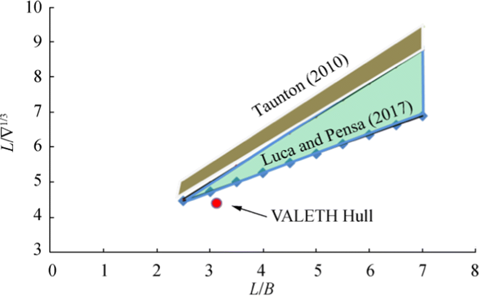Figure  1  Typical range of the non-dimensional parameters for planing hulls

Download: Full-Size Img

2.1   Resistance Test Setup and Procedure

Planing hull model tests require a setup to facilitate the dynamic trim and emergence of the hull form. The model tests are performed at the towing tank facility at the Department of Ocean Engineering, IIT Madras. The tests follow the recommendations as in ITTC procedures 7.5-02-05-01 for high-speed marine vehicles (HSMVs), which are based on the 1978 prediction method. The tank dimensions are 82.0 m × 3.2 m × 2.5 m (water depth), and the maximum towing carriage speed is 5 m/s. The towing carriage has precision selectable speed control and automation to simulate the steady-speed dynamic conditions of the tests.

The test setup provides a selectable sliding pivot point to facilitate the model to take its natural trim during towing at steady speed; see Figure 2. It consists of a precision linear guide system for friction free sinkage or emergence of the model, a pivot mechanism with bearings for natural dynamic trim of the model, load cell for resistance measurement and counter-weight mechanism to control model displacement. The details of the experimental setup used for this study are given in Rakesh et al. (2018). The model is manufactured to high accuracy using rapid prototyping based on the 3D CAD representation of the hull. This provides for accurate modelling of the chines and spray rails. No turbulence stimulator is used in the test of high-speed crafts as per the ITTC guidelines. A motion reference unit (MRU) measures the dynamic trim. The dynamic wetted surface and waterline length are estimated from video recordings of the runs. The screenshots from the video recordings for a speed are scanned to map the wetted portion of the hull to the CAD model using the reference lines marked on the physical hull. The surface area of the wetted portion of the hull and the waterline length are estimated from the CAD model. The resistance of the model is scaled to prototype values using a method applicable for planing vessels using the ITTC 57 friction correlation line.

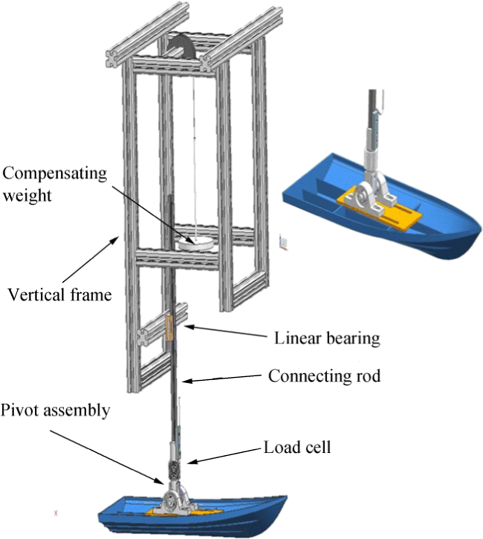Figure  2  Experiment setup for high-speed model tests, in Rakesh et al. (2018)

Download: Full-Size Img

Figures 3, 4 and 5 bring out the nature of transition in the pre-planing region for the same hull form with different L/∇^1/3. The displacement is changed using calibrated weights placed inside the model, and zero static trim is maintained as per the initial design across the loading conditions. For the light hull-weight ratio of 6.0, the hull form manifests a smooth behaviour at transition speeds (see Figure 3) of 12, 13 and 14 kn before achieving full planing ultimately. For the hull-weight ratio of 5.0, in Figure 4, the transition behaviour is again smooth. For the hull-weight ratio of 4.42, which is characteristic of heavier-than-normal displacement, Figure 5 shows the wave pattern in displacement mode at a low speed of 6 knots. Figure 6 shows heavy spray at the bow at the transition speeds of 12, 13 and 14 knots, though eventually, the vessel emerges with relatively clean planing and a more visible wave pattern at 16 kn. The objective in this study is to model the transition behaviour numerically for the heavier hull-weight ratio of 4.42 for early assessment of the design. Development of a reliable analytical tool will help avoiding costly and time-consuming physical experiments. The focus of interest is the pre-planing behaviour and its prediction.

Figure  3  Planing at 12, 13 and 14 kn for L/∇^1/3 = 6.0; note the smooth transition

Download: Full-Size Img

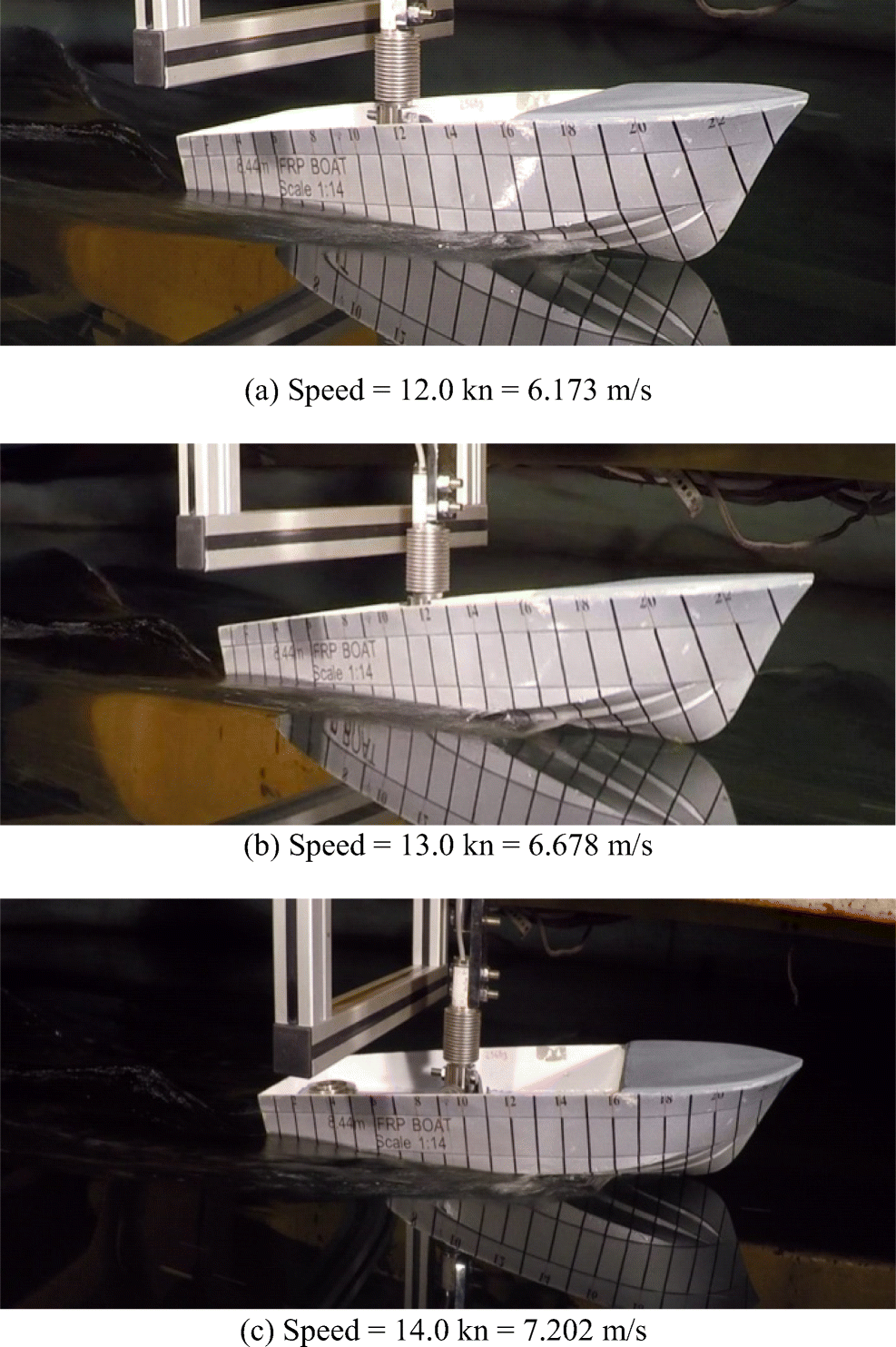Figure  4  Planing at 12, 13, 14 knots for L/∇^1/3 = 5.0; note the changing wave pattern

Download: Full-Size Img

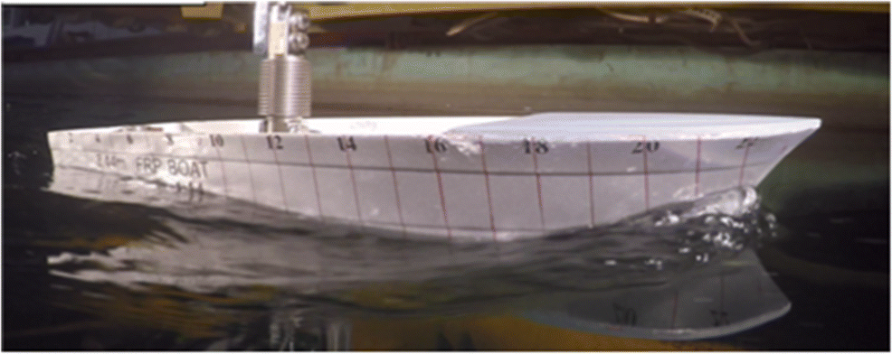Figure  5  With heavier-than-normal displacement L/∇^1/3 = 4.42, prominent wave pattern at lower speed 6.0 kn = 3.086 m/s

Download: Full-Size Img

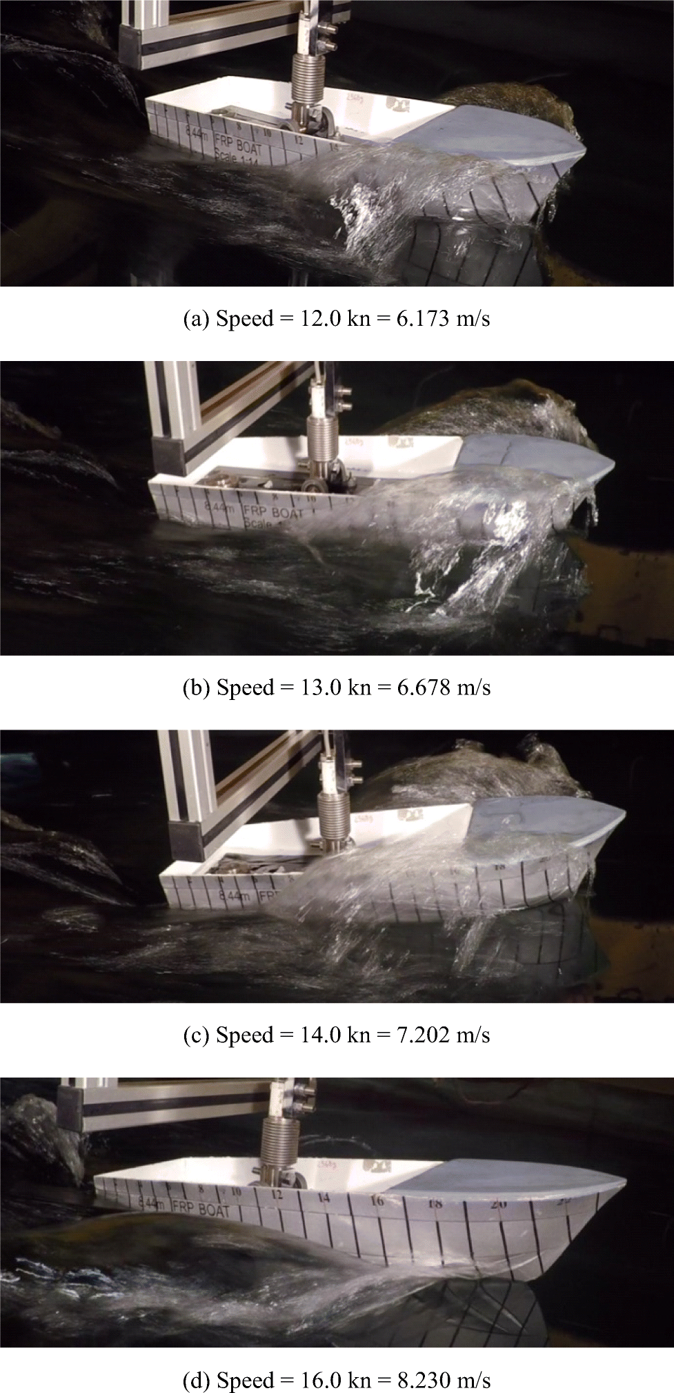Figure  6  For L/∇^1/3 = 4.42, planing attained after heavy spray in the pre-planing region

Download: Full-Size Img

3   Numerical Simulation of Planing Hull

The methodology consists of exploring numerical modelling with different mesh topologies of the fluid medium and the air–water interface. First, the comparison is made with the results for drag, waterline length and dynamic trim as obtained from the Savitsky scheme. The values are also validated with experimental data. To facilitate direct comparison with the model test results, the numerical modelling was carried out at model scale, which is 1:14.0.

3.1   Numerical Modelling

A commercial RANSE-based code (Star-CCM+ v11.06.010) is used in the simulation of flow at different speeds to obtain the dynamic equilibrium with lift, dynamic trim and drag forces. The objective is to simulate the kinematic aspects of flow including the bow wave pattern, spray resulting from air–water interaction effect and effective dynamic wetted length besides obtaining the dynamic trim and the drag at steady speed. Obtaining all these parameters reliably requires a suitable modelling strategy.

One of the critical components in the methodology is the choice of the proper multiphase model to simulate the wave and spray. The use of the two-phase VOF model with a modified high-resolution interface-capturing (HRIC) scheme for immiscible fluids allows solving a single set of conservation equations for mass, momentum and energy for an equivalent fluid phase. The fluid properties such as density and viscosity are calculated based on the corresponding properties of the constitute phases and their volume fractions. The stock HRIC scheme can be modified to blend downwind and upwind schemes for improved stability based on the upper and lower limits set for the local Courant–Friedrichs–Lewy number (CFL). The modified scheme has improved stability to simulate complex free surface flows with associated disadvantage to reduce interface resolution which will lead to numerical ventilation as indicated in De Luca et al. (2016). Hence, care is taken in setting the CFL limits, and mesh refinement zones are created where the free surface is expected as described in the following sections.

In order to capture the flow phenomenon, the domain boundaries within which the computation grid is modelled are extended to 2L (where L is the length of the ship) in front of the bow, 5L behind the transom and 2L above the deck, below the keel and to the side of the hull. These dimensions are consistent with the recommendations given in ITTC 7.5-03-02-03. Due to the centreline symmetry of the ship as well as the flow, only half the hull is included in the domain. The analysis process considers the dynamic emergence and dynamic trim based on the two-degree-of-freedom motions in the vertical plane along the hull.

The spray rail is modelled placing four to six cells along its width to analyse the flow field. Prism layers are generated adjacent to the hull surface to generate high-quality mesh required to capture the viscous effects in the boundary layer; the prism mesh parameters are chosen such that the average wall y+ achieved on the hull is around 50, based on Azcueta (2003). A mesh refinement zone is used near the free surface to capture the waves generated by the ship with a minimum of 80 cells per transverse wavelength in the longitudinal direction and 40 cells per wave height; this is achieved by selecting the lowest speed in the study as the basis for refinement, and the mesh is valid for other higher speeds. A separate refinement zone is used in the forward region of the hull, overlapping the free surface refinement zone, to capture the bow wave. The time step interval is specified such that the Courant number is less than 1 for all the simulations; hence, finer grids require smaller time steps. The inlet velocity, for both air and water phases, is specified as a constant value equal to the ship speed in the simulation. The pressure outlet boundary downstream of the ship is specified as hydrostatic pressure considering the still water surface, and the volume fraction field is set to the volume fraction of the free surface.

3.2   Meshing Strategy

The mesh parameters directly influence the accuracy of the numerical results. Three different types of grids have been used, and the values of resistance and dynamic trim have been obtained in each of these cases for comparison.

In the single-grid method, the response of the hull due to fluid forces in terms of translation and rotation is calculated with respect to an inertial/fixed frame of reference. Hence, the position and orientation of the simulation domain, defined by the boundaries and the mesh surrounding the hull, change with respect to the fixed frame of reference. This causes difficulties with convergence and accuracy of the multiphase flow simulations with large motions, as the general flow direction and shape and orientation of the interface change with reference to the mesh; see Figure 7.

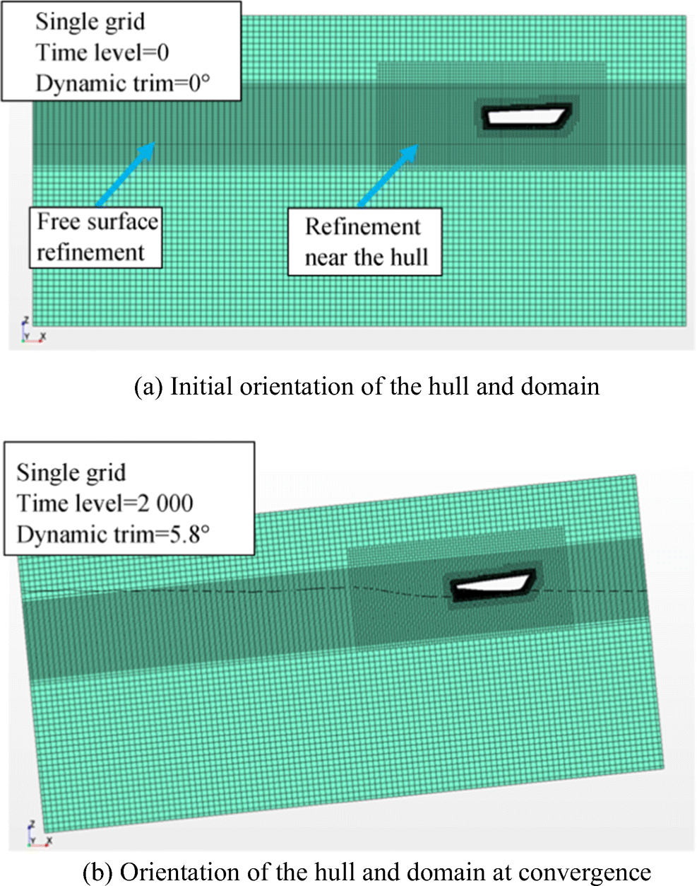Figure  7  Initial and converged orientations of the hull and domain in a single-grid system respectively

Download: Full-Size Img

Refined mesh is used in the regions around the hull, in the wake of the hull and at the free surface as shown in Figures 8 and 9. The refinement blocks are strategically placed in the regions of the domain where the flow gradients are high. In the case of single grid, the alternate method for rigid motion of the mesh is the morphing technique, which redistributes the mesh vertices in response to the movement of the surface. The mesh is updated by calculating the node coordinates between time steps and parameters such as skewness; the aspect ratio varies with solution time depending on the body movement. However, this method is most appropriate for scenarios where components deform or changes their shape (Kang and Lee 2010; Biancolini et al., 2014).

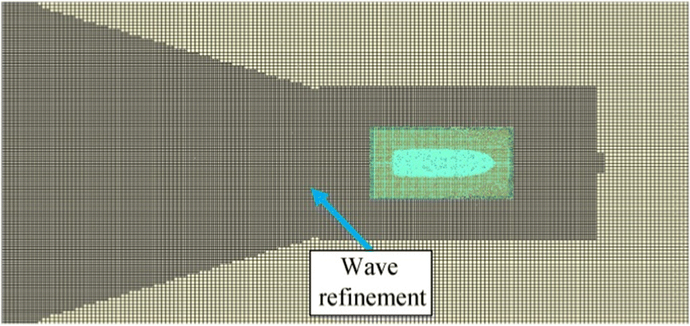Figure  8  Free surface refinement shown in plane parallel to still water surface

Download: Full-Size Img

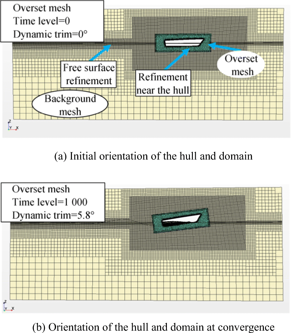Figure  9  Initial and converged orientations of the hull and domain in an overset system respectively

Download: Full-Size Img

To improve the convergence and accuracy of the simulations, the overset mesh is used which has two different mesh regions namely an overset mesh and a background mesh (static mesh), shown in Figure 9a. The overset mesh along with the hull moves over a static background mesh of the whole domain. This also creates sufficient grid refinement in the free surface and saves computational time while improving the accuracy. The meshes in the initial and converged states of the simulation are shown in Figure 9 a and b respectively.

The overset mesh computations suffer from interpolation errors in the dependent variables at the grid interface, and this results in mass imbalance across the overset boundaries (Hadzic 2006). The effect of inherent non-conservation of mass on the solution is minimized by appropriately choosing relatively small dimensions for cells in the overlapping regions of the grid.

The overset mesh method itself has two types of gridding schemes; therefore, altogether, three mesh schemes have been adopted:

1) Single grid consisting of trimmed grid cells and referred to as SG

2) Overset mesh consisting of trimmed grid cells (both background and overset regions) and referred to as overset TT or (OTT)

3) Overset mesh consisting of trimmed grid cells (background region) and polyhedral grid cells (overset region) and referred to as overset TP or (OTP)

The time step is initialized with a guessed value according to the ITTC recommendation which is a function of the hull speed and wetted keel length (L_k) from the following equation:

During the simulation, the time step is modified as necessary to fulfil the Courant number criterion (< 1.0), which is based on grid spacing and flow velocity.

The solution convergence requires five to ten iterations per time step (called inner iterations) at the end of which the root mean squared (RMS) residual (for the continuity, momentum, and turbulence and VOF equations) drops by three orders of magnitude. The details of the iterative convergence and uncertainty are given in Section 3.3.

The boundary conditions and solver settings used in the simulations are given in Tables 3 and 4.

3.3   Verification and Validation of Simulations

3.3.1   Verification Procedure

The verification and validation study of the CFD simulations are performed based on the methodology prescribed in McHale et al. (2009), Coleman and Stern (1997) and Stern et al. (2001). Verification is defined as a process (Biancolini et al., 2014) of assessing simulation numerical uncertainty U_SN based on estimating the simulation numerical error (δ_SN) itself and the uncertainty in that error estimate. Verification analysis is performed independently for SG, OTT and OTP mesh methods. The verification is carried out for the response variables, namely total resistance coefficient, pressure resistance coefficient, wetted surface area and dynamic trim at a design speed of 25 kn that corresponds to 3.437 m/s for the model.

The numerical uncertainty U_SN is composed of iterative U_I, time step U_T, grid uncertainties U_G and the statistical errors U_P. In this work, two methods are employed to combine the components for determination of U_SN.

RMS addition: Based on Stern et al. (2001), the combined numerical uncertainty is estimated by RMS addition given by

Arithmetic addition: As per McHale et al. (2009) and Eça and Hoekstra (2009), the combined numerical uncertainty is estimated by arithmetic addition given by

3.3.2   Grid, Iterative and Time Step Uncertainty

The grid convergence studies are performed for each mesh (SG, OTT and OTP) using three progressively refined grids called grids A, B and C, which are coarse, fine and finest respectively. The number of cells is given in Table 5, and the respective time step used is listed in Table 6. Due to the use of unstructured and overset grids, the cell count for each successive refinement is increased by a factor of approximately √2 based on De Luca et al. (2016), which results in a slightly lower value of the refinement ratio 2^(1/3) = 1.26 for cell edges than the recommended range between √2 = 1.414 and 2 in the ITTC guidelines. Crepier (2017) discussed unstructured grid refinements based on geometric similarity using the anisotropic sub-layer method. In the present work, progressively refined grids are generated based on the refinement factor; however, the prism mesh parameters namely the first cell distance normal to the wall and stretching are prescribed which results in geometrically similar cells. For grid B, ten layers of prism cells are used adjacent to the hull.

Figure 10 shows the wall y+ for the finest grid, i.e. grid C in each of the three mesh types, for the maximum speed of 25 kn. The cell parameters in the prism layer mesh are chosen based on the wall y+ requirement for proper turbulence modelling. The turbulence parameters are constant for all the grids A, B and C. The wall y+ values are in the range of 30–130 over the hull and independent of the core mesh refinement. Table 7 shows the average values of wall y+ for the three different meshes on the hull at the maximum speed of 25 kn.

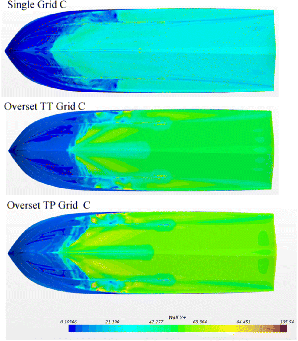Figure  10  Contour plots of wall y+ (0.10 to 105.54) at 25 knots for the finest grids

Download: Full-Size Img

The response variable S_W representing the wetted surface is estimated using the distribution of the volume fraction of water (α) over the hull surface; see Figure 11. It is given by the sum of area of the cells on the hull surface with a volume fraction α greater than 0.5. The alternate approach for the estimation of S_W is to calculate the surface integral of α over the hull surface; the comparison error based on the two approaches is 2.5%, and this indicates that the effect of numerical ventilation is marginal for OTT and OTP mesh. For the case of SG mesh, the comparison error is larger than the other meshes due to the cells in the free surface zone region being not aligned to the free surface.

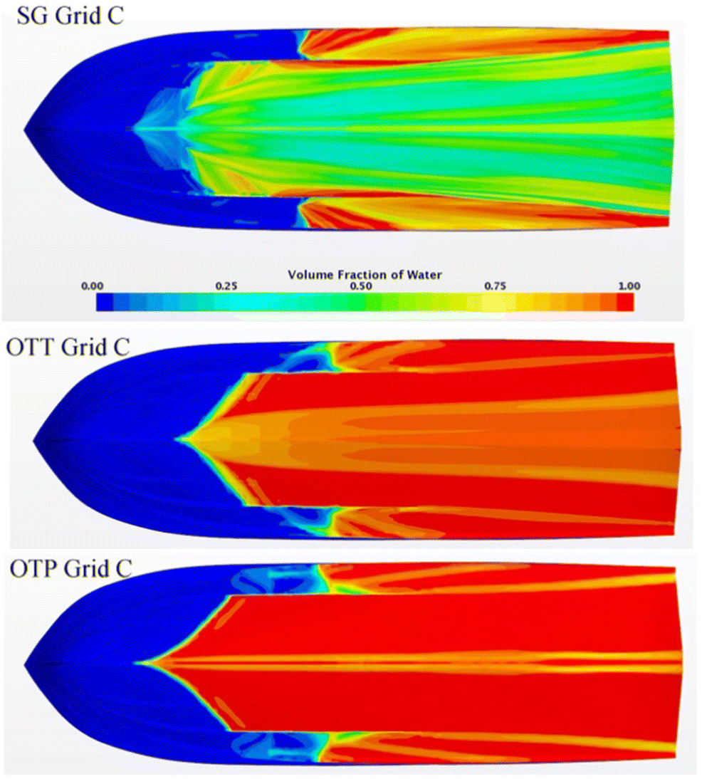Figure  11  Volume fraction of water shows the wetted area on the hull for three different meshes at 25 kn

Download: Full-Size Img

The data obtained from grid dependency analysis is given in Table 8; the analysis uses the correction factor method from Stern et al. (2001). It is established that the condition for monotonic convergence is achieved since for all the response variables considered, the grid convergence ratio (R_G) is less than 1. The grid uncertainty parameter (U_G) shows that the grid sensitivity is moderate for the OTP compared with other meshes. The sensitivity is more significant for C_T with OTT mesh.

The statistical convergence is estimated by calculating the difference of the mean obtained from the time history of the response variable in the asymptotic window with the mean in the last oscillation. The running mean of oscillations is less than 0.84% of the mean value for all response variables across the cases.

Inner iterations are performed for convergence of solution in each time step, and the iterative uncertainty is measured defined based on the oscillatory iterative convergence described in Stern et al. (2001). U_I was not mainly influenced by the resolution of the grid (Xing et al., 2008). Table 9 shows the iterative uncertainty for all the response variables using grid B at a speed of 25 kn. The results show that the variation of the response variables using the OTT mesh and OTP mesh is less than 1% by increasing the number of iterations from five to ten. For SG mesh, the variation of response variables is about 2%, and it is more sensitive to the variation of inner iterations. This study executes the simulations with ten inner iterations.

To obtain the time step uncertainty, this study generates three solutions using the ratio of √2 between succeeding time steps. The study performs simulations using corresponding grid B in each of the three cases, namely SG, OTT and OTP. Table 10 gives the results, which show that the convergence ratio (R_TS) is less than unity, indicative of monotonic convergence towards the time step. The time step uncertainty for C_T and C_P is less than 0.5% for all the three cases of the meshes, and the dynamic trim τ and wetted surface area S_W are relatively more sensitive with regard to time step for OTP and SG respectively.

The individual uncertainties for each of the three different mesh types are given in Table 11. The combined uncertainty U_SN based on the two different methods—RMS addition and arithmetic addition—are given in Tables 12 and 13 respectively. From Table 11, it is observed that U_G is mostly greater than U_I though not different in order of magnitude; hence, the iterative and grid errors are not uncorrelated. As described in McHale et al. (2009), the statistical assumption to use RMS addition is not strictly valid. Comparing corresponding magnitudes of U_SN in Tables 12 and 13, RMS addition results in a lower value of U_SN compared with arithmetic addition. It is evident that RMS addition results in overly optimistic combination, as suggested more recently by Eça and Hoekstra (2009); arithmetic addition is more conservative and reliable in estimating numerical uncertainty. For the validation of simulations discussed in the following section, the arithmetic addition–based U_SN is used. Using a higher refinement ratio poses some issues in this case-specific modelling of the high-speed planing hull form using unstructured and overset grid, with the additional requirement of introduction of a refinement zone at the air–water interface to capture spray. Owing to the nature of the craft, the significant emergence and trim lead to change of the free surface position in relation to the grid, resulting in poor convergence due to the lack of grid resolution in coarser grids to capture similar flow physics when using higher refinement ratios. For this reason, the investigation here uses the refinement ratio 1.26. In this background, the use of the arithmetic addition–based (less stringent than the RMS based) uncertainty analysis gives a more conservative estimation for validation. From the combined uncertainty, U_SN for each response variable is less for OTP mesh compared with those for the two other meshes.

For grid B, Figure 12 shows the number of time steps required to achieve convergence for the three mesh types; the rate of convergence is highest for OTP followed by that for OTT. The solver time required for OTT simulations to achieve convergence with grid C is 44 h by employing four CPU cores.

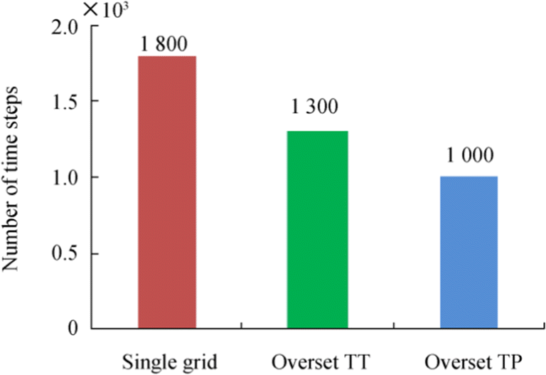Figure  12  Number of time steps required to achieve convergence in C_T obtained using grid B for 25 kn

Download: Full-Size Img

An attempt is made to compare the verification results from the present study and De Luca et al. (2016); the corresponding results from the later work are given in Table 14 for OTP mesh which is the only common mesh type for both the studies. It is to be noted that L/B is 2.81 for the hull used in the current work and 3.45 for the hull used in the reference (De Luca et al. 2016). The corresponding Froude numbers are 1.50 and 1.44. Therefore, the hull employed for the present study is relatively slender and slightly 'faster'. The grid (U_G), iterative (U_I), time step (U_TS) and simulation numerical (U_SN) uncertainties are given for three response variables namely the total resistance coefficient, dynamic trim and wetted surface area. De Luca et al. (2016) used four grids (progressively refined D–A–C–B) to determine two different grid (U_G) uncertainties using D–A–C and A–C–B, and both the values are given here.

From the data in Tables 11, 12 and 14, it is evident that the corresponding uncertainties for each of the response variable are numerically different when compared between the two separate sets of investigations. Lower values are reported for (U_G), (U_I) and (U_SN) by the present work compared with the corresponding values of De Luca et al. (2016) while (U_TS) values are higher from the present work across the three response variables.

Use of relatively fine mesh with a larger cell count in the present study could be one of the reasons for obtaining lower uncertainties compared with De Luca et al. (2016). (U_I) and (U_TS) are obtained using intermediate mesh in the present study while De Luca et al. (2016) used the coarsest grid. As concluded by De Luca et al. (2016), the uncertainties are also dependent on the hull slenderness.

3.3.3   Validation

The validation of simulations follows the method based in Stern et al. (2001) based on the estimation of error between simulation result (S) and experimental data (D), namely the comparison error (E) and the validation uncertainty (U_V):

Here uncertainty U_V is the combination of experimental uncertainties (U_D), simulation uncertainties (U_SN) and input uncertainty (U_input). Simulation error and uncertainty have components from modelling, numerical and input elements. The modelling error is due to assumptions and approximations of the simulation model in representing the physical phenomena. The numerical error is introduced due to numerical computations based on the governing equations, and input error is due to the errors in the simulation input parameters.

The uncertainty in the input data is related to the body geometry and fluid parameters such as density and viscosity. It is assumed that the input uncertainty is negligible in comparison with other numerical uncertainties.

If │E│ < U_V, i.e. the error lies within the validation uncertainty, then the validation is achieved for this uncertainty level.

If │E│ > U_V, i.e. the error lies outside the validation uncertainty, then validation has not been achieved for this uncertainty level, and therefore, there is a need for improving the simulation modelling.

As per the recommendation of ITTC 7.5-02-02-02.1, the uncertainty analysis for the towing tank test shows that the errors are mainly due to the quality of the load cell measurement, to repeatability of the tests and to a very small extent to variation in the speed of the model and water temperature. The other uncertainties due to model manufacture and installation are assumed negligible in this study. Seven test runs were conducted to estimate the uncertainty for repeatability of experiments, and the measured quantities are given in Table 15. Uncertainty is obtained from mean of the runs; the percentage of standard deviation for resistance is 1.77. The uncertainty in the load cell measurement and repeatability of experiment is therefore 1.22% and 0.67% respectively, and the combined uncertainty is 1.34%. Further, with 95% confidence level, the total uncertainty for the measurement of resistance (U_D) is 2.68% (± 0.14 N), and the corresponding values for wetted surface area and trim are 0.40% and 0.35% respectively.

The data required for validation of the three mesh schemes are given in Figure 13, which consists of the error E and uncertainty in validation U_V for each response variable, namely total resistance, pressure resistance, wetted surface area and dynamic trim respectively. The numerical uncertainty U_SN based on the conservative arithmetic method is used for calculating U_V. It is observed that validation is achieved for all the response variables for OTT mesh. For OTP mesh, the validation is achieved for all the response variables except for the pressure resistance coefficient. For SG, mesh validation is achieved only for the wetted surface area.

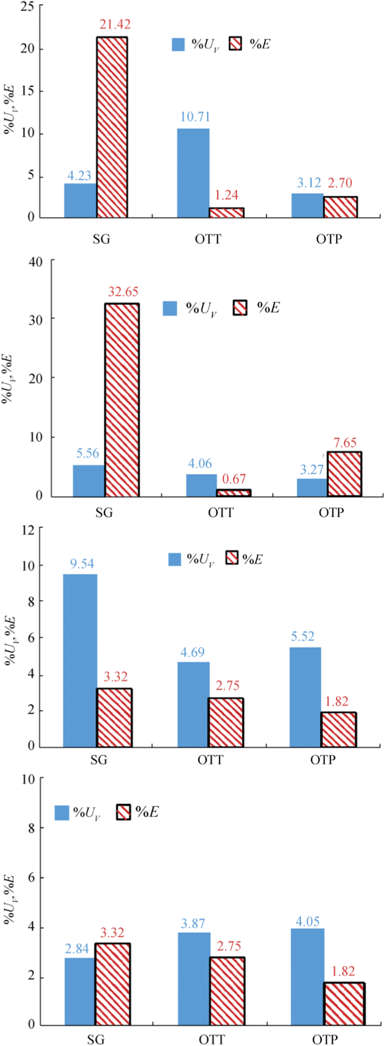Figure  13  Representation of validation uncertainty (U_V) and comparison error (E) for the different meshes

Download: Full-Size Img

The level of validations achieved is as follows:

• For SG, U_V = 9.5%D for S_W

• For OTT, U_V = 10.7%D, 4.1%D, 4.7%D and 3.9%D for C_T, C_P, S_W and τ respectively

• For OTP, U_V = 3.1%D, 5.5%D and 4.1%D for C_T, S_W and τ respectively.

With reference to Figure 13, the comparison errors for OTT and OTP meshes are far less compared with those of SG; therefore, the overset-based meshes give more reliable prediction of the planing hull performance. However, the difference between comparison errors for OTT and OTP is less compared with the combined uncertainty in validation. Therefore, this does not indicate the better method in relative terms, though the comparison error is smaller in the case of OTT as against that in OTP.

4   Evaluation of Results from Different Methods

4.1   Prediction Using Savitsky Method

The empirical method for planing hulls due to Savitsky (1964) is based on systematic tests using prismatic models considering dead rise angle, length to beam ratio and trim. To predict the resistance and running attitude, the method assumes that, for prismatic hull forms in calm water, the resultant hydrodynamic force acts through the centre of gravity. The total resistance of the planing hull is due to pressure resistance (R_P) and viscous resistance (R_V).

Figure 14 shows the results for drag, waterline length and dynamic trim as obtained for different mesh configurations from the CFD simulations compared with the Savitsky scheme–based results. At the design speed of 25 knots, the comparison errors in total resistance and dynamic trim by the Savitsky method are 9.5% and 20% respectively as compared with the OTT mesh–based simulations.

Figure  14  Results of different mesh configurations compared with the Savitsky method

Download: Full-Size Img

4.2   Experimental Results

The experiments were conducted to compare the results from the different numerical schemes as well as from the Savitsky scheme. Figures 15 and 16 show comparisons of wave patterns at planing and pre-planing speeds respectively. The prominent wave pattern at the aft and the wave at the fore-body are clearly brought out in the CFD simulation and compared well with the pattern captured from the experiments. Figure 17 shows the wave pattern at progressively increasing speeds of 8, 12 and 25 kn.

Figure  15  Experiment and simulation using overset TT at full planing speed (25 kn)

Download: Full-Size Img

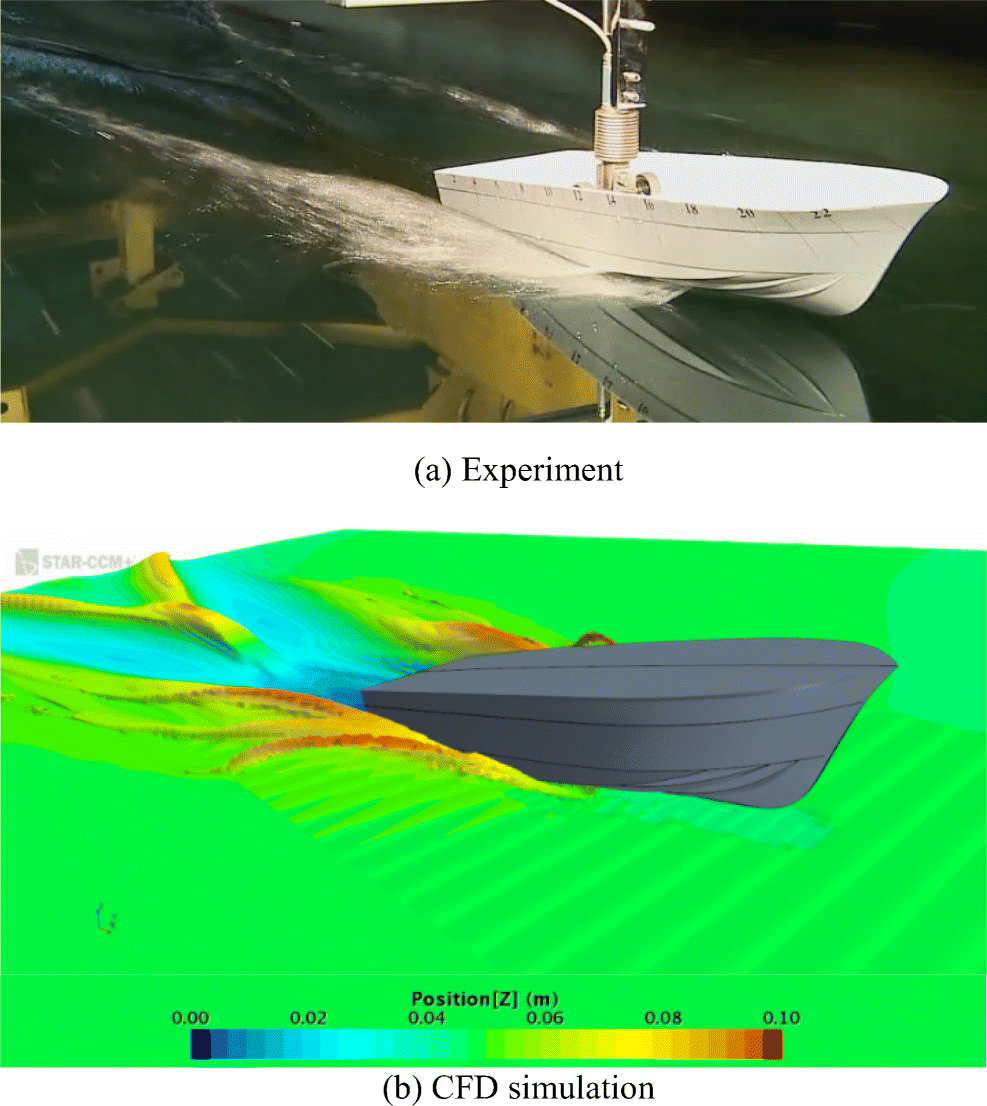Figure  16  Experiment and simulation using overset TT at pre-planing speed (8 kn)

Download: Full-Size Img

Figure  17  Wave pattern generated by the hull at different speeds

Download: Full-Size Img

Figure 18 is an underwater video frame, which shows the underwater contact area and wave pattern at the design speed. Figure 19 shows the comparison obtained from the OTT-based simulation. Both images show the separation of flow at the anti-spray rails.

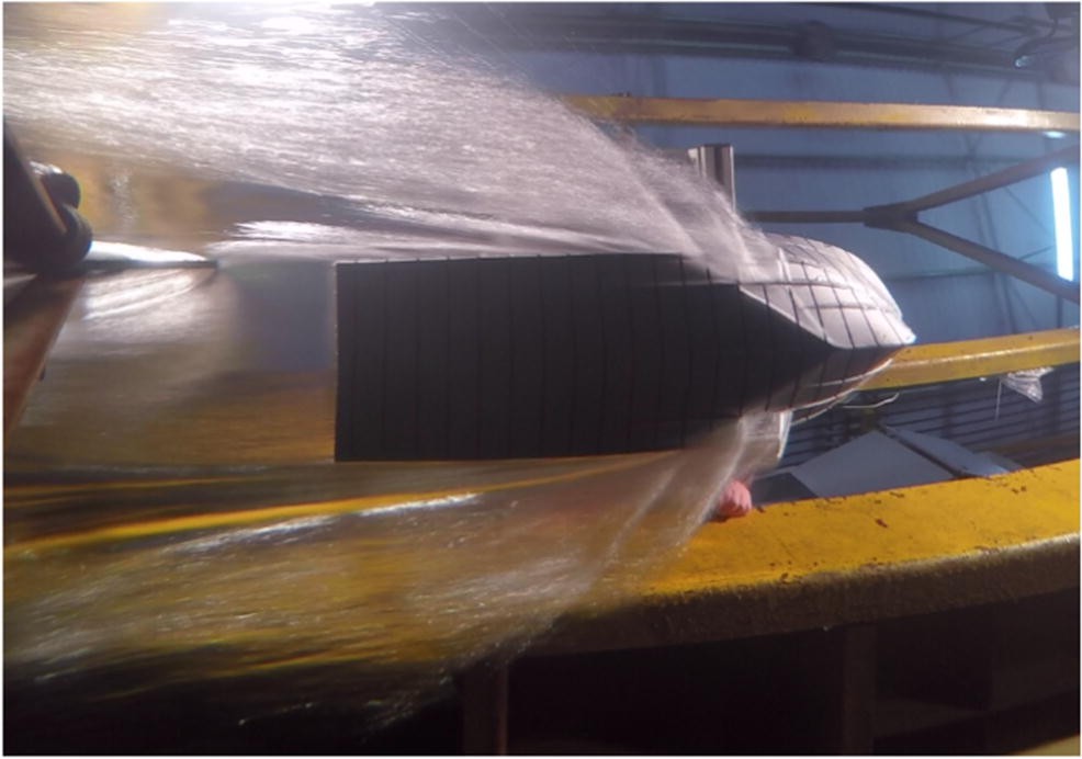Figure  18  Picture taken from the underwater camera at design speed of 25 kn

Download: Full-Size Img

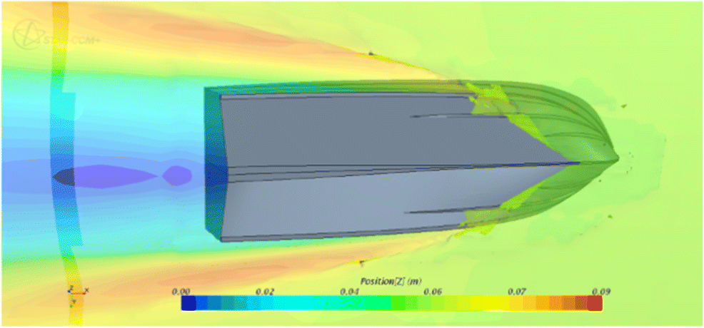Figure  19  Visualization of underwater using overset TT simulation at design speed of 25 kn

Download: Full-Size Img

4.3   Spray

The formation and breakup of the turbulent fluid flow layer associated with the generation of bow spray is obviously a complex multiphase flow problem. To improve the details of the spray captured, simulations use an increased sharpening factor of the HRIC which reduces numerical diffusion. Particularly for pre-planing speeds to capture the bow wave and improve the resolution of the interface between phases, a sharpening factor closer to 1 is used. Higher limits are set for lower and upper CFL to remove the dependency of the modified HRIC scheme on local CFL which will, as discussed in De Luca et al. (2016), minimize smearing of the free surface and reduce numerical ventilation. The details of VOF solver and HRIC parameters are given in Table 16.

Figure 20 shows the instantaneous picture of bow wave formation. Figure 21 shows the same as generated by the OTT mesh–based simulation. Figure 22 shows transverse sections at the forward region to capture the growth of the spray along the vessel length at the pre-planing speed. Figures 23 and 24 show the orientation of the free surface with the grid lines for SG and OTT. It is observed that the free surface is largely aligned to the grid for the overset mesh, which results in sharp capturing of the interface, compared with single grid.

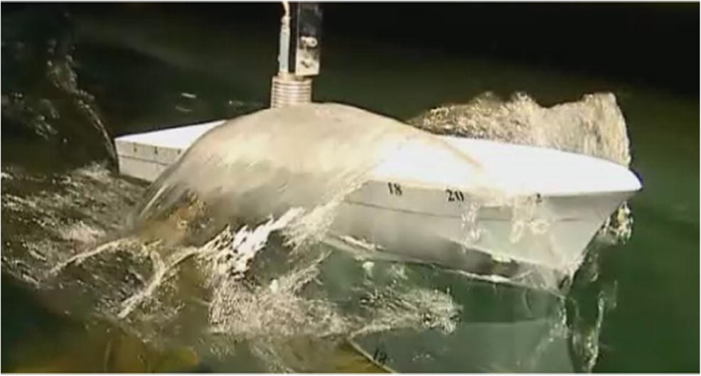Figure  20  Bow wave spray from experiment at 14 kn

Download: Full-Size Img

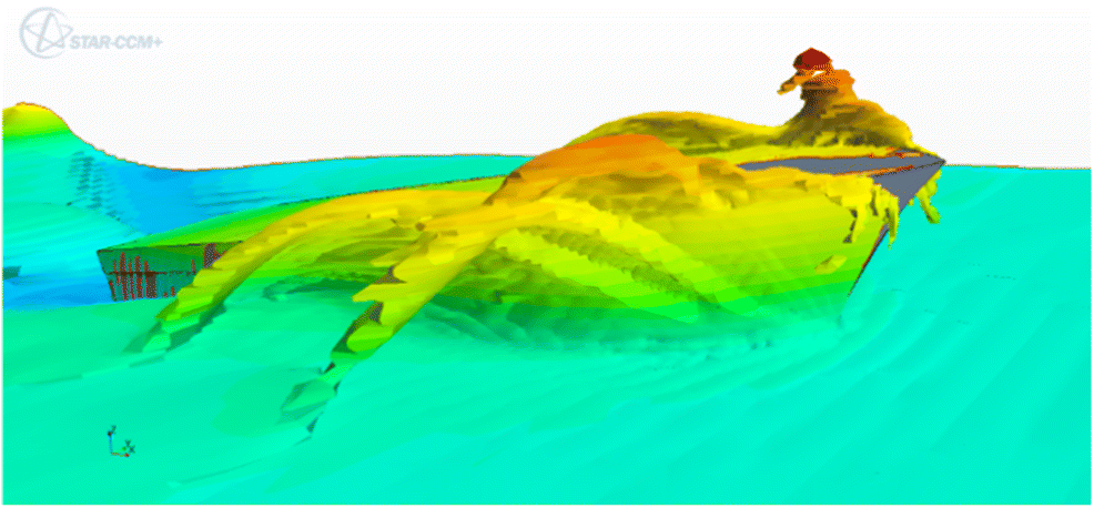Figure  21  Large bow wave spray generated at the transient speed of 14 kn—experiment and overset TT simulation

Download: Full-Size Img

Figure  22  Spray generation at different transverse sections (with distances from the transom) at transition speed of 8 kn

Download: Full-Size Img

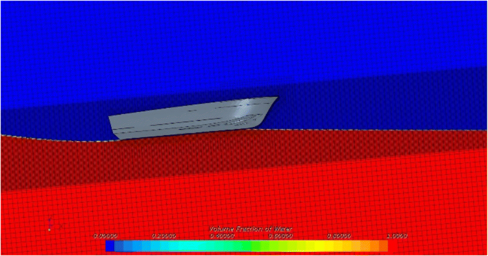Figure  23  Volume fraction of water showing the non-alignment of free surface and the grid lines in SG

Download: Full-Size Img

Figure  24  Volume fraction of water showing the undisturbed free surface aligned to the grid lines in OTT

Download: Full-Size Img

Figure 25 gives the summary of results obtained from the simulation using the three different mesh types and from experiments for a range of speeds. De Luca et al. (2016) presented similar results for different vessels with L/B between 3.45 and 6.25 for Froude number range of 0.82 to 1.44 while the current vessel has an L/B ratio of 2.81, and the range of Froude number investigated is between 0.6 and 1.5. Observations are consistent between the former and present work as the comparison of the qualitative trends indicate, especially for total resistance and running trim with speed. All computational results using overset mesh are generally in good agreement with experimental data (Figure 26). The error for total resistance significantly increases with speed for SG as compared with OTT and OTP. For SG mesh, the total resistance is in good agreement with experiments at the lower pre-planing speeds. At the planing speed, the hull significantly lifts up with attendant change of running attitude and the results show large deviation of the total resistance as compared with experimental data.

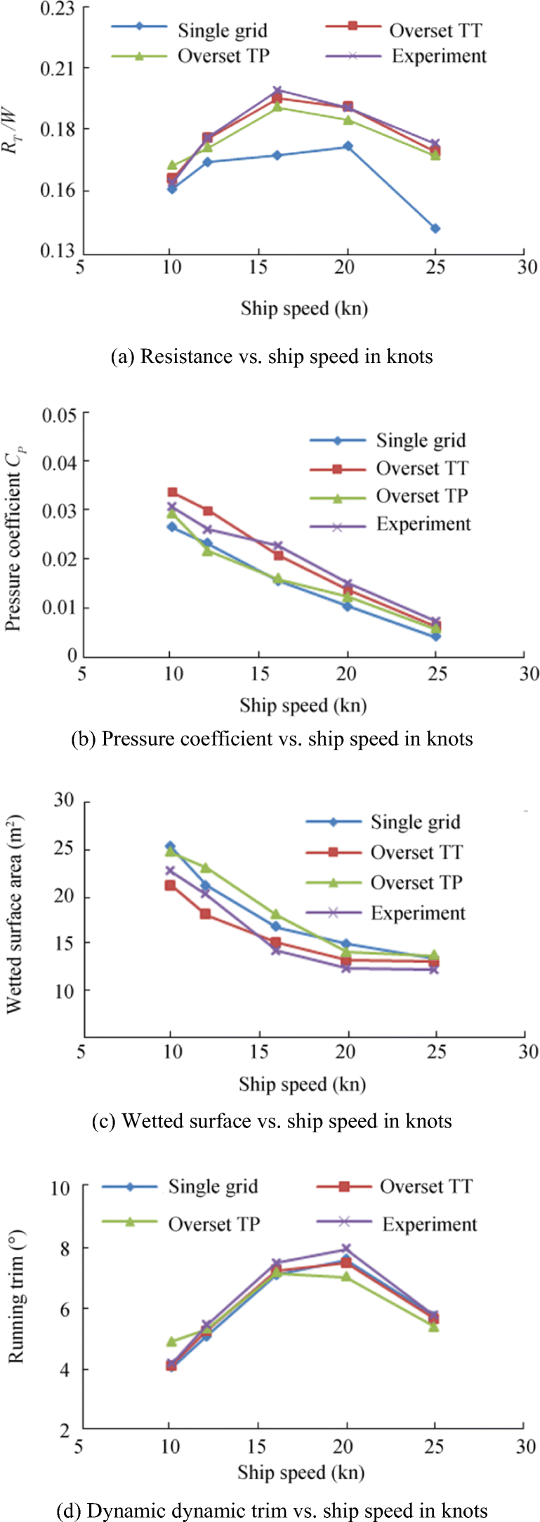Figure  25  Comparison results by the different meshes and experiment

Download: Full-Size Img

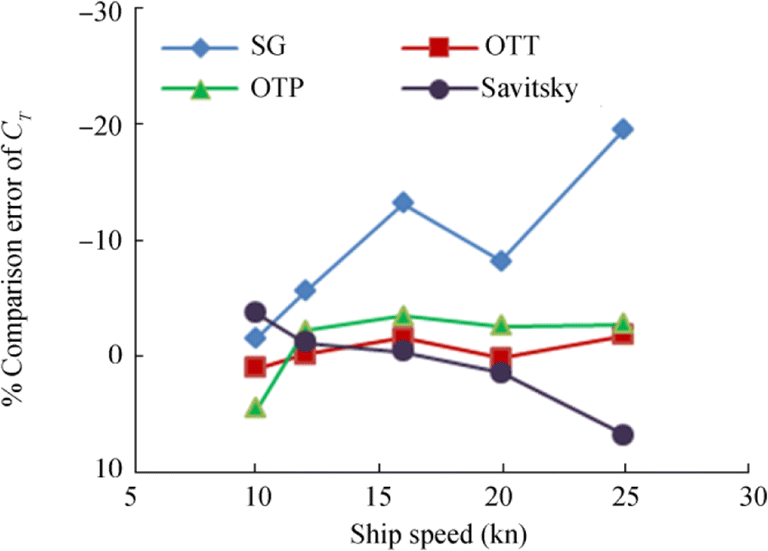Figure  26  Comparison error of total resistance of different mesh configurations and the Savitsky method with respect to experiment

Download: Full-Size Img

5   Conclusions

The study establishes that the overset grid yields good simulation results for the high-speed loaded planing hull with a low length to displacement ratio and captures the kinematics much better in comparison with the single-grid mesh approach. The single-grid mesh is not suitable for the larger motion characteristics of the planing hull where large emergence and trim changes occur with speed. Though the trends in the performance parameters are estimated well by the Savitsky method over the speed range studied, the comparison errors are more in the pre-planing region. The comparison with experiments conducted in the towing tank establishes that the complex multiphase flow is realistically captured from the numerical simulations based on overset meshes. The associated dynamic trim, waterline length and resistance of the hull form obtained using overset mesh are much closer to the values as measured from the experiments. The methodology for numerical simulations described here is a valuable procedure for early stage design verification. It provides valuable assessment of the design bringing down the necessity to conduct complex costly and time-consuming experiments in a towing tank.

Nomenclature