1   Introduction

The liquid motion in vessels and containers is called sloshing. The motion of walls is transferred to the liquid, a process categorized as fluid–structure interaction (FSI). Currently, the interaction between fluid and structures is an important problem in several industries. Pumps, turbines, airplanes, and ships are examples of systems with FSI problems. To investigate this problem, experimental and numerical methods are used. Eulerian and Lagrangian numerical methods have been applied to simulate FSI problems. Eulerian methods are usually grid-based; therefore, the motion of a solid body grid is defined and imposed during any iterations.

One of the most important problems in the free-surface flow is liquid sloshing in tanks, which is a well-known phenomenon in liquid transport tanks. Sloshing may create great forces and momentums, and consequently, controlling the tank and its carrier becomes difficult and unsafe. Hence, predicting and controlling the sloshing phenomenon are essential to the liquid transport industry.

Valuable studies have been conducted in this field.Shadloo et al. (2016) simulated breaking and non-breaking long waves using the smoothed particle hydrodynamics method and investigated the effectiveness of a certain turbulence model for violent free-surface flows. Kim et al. (2012) investigated a comparative study on model-scale sloshing tests. Kim et al. (2015) comparatively studied pressure sensors for measuring sloshing impact pressure. Ming and Duan et al. (2010) proposed a method for the simulation of sloshing in a sway tank, in which the two-phase interface is treated as a physical discontinuity that can be captured by a well-designed high-order scheme. Ozbulut et al. (2018) simulated a two-dimensional oscillatory motion in partially filled rectangular tanks using the smoothed particle hydrodynamics method; the governing equations were discretized with velocity variance-based free-surface and artificial particle displacement algorithms. The authors investigated the effects of tank geometries, fullness ratios, and motion frequencies. Shamsoddini and Abolpur (2019) modeled shallow water sloshing in a rectangular tank by an improved turbulent incompressible smoothed particle hydrodynamics (ISPH) method. Deshpande et al. (2012) evaluated the performance of an open-source multiphase flow solver. The solver was based on a modified volume-of-fluid (VOF) method, which included an interfacial compression flux term to moderate the effects of numerical smearing of the interface. Hou et al. (2012) simulated liquid sloshing behavior in a two-dimensional rectangular tank using OpenFOAM software. Godderidge et al. (2009) modeled sloshing flow in a rectangular tank with a commercial computational fluid dynamics (CFD) code. Chen and Price (2009) developed a numerical scheme to model compressible two-fluid flows simulating liquid sloshing in a partially filled tank. Zhao et al. (2018) developed a numerical code based on the potential flow theory to investigate nonlinear sloshing in rectangular liquefied natural gas tanks under forced excitation. Using this code, internal free-surface and sloshing loads on liquid-cargo tanks can be achieved both in time and frequency domains. Saghi and Ketabdari (2012) developed a numerical code to model liquid sloshing in a rectangular partially filled tank. To minimize the sloshing pressure on tank perimeter, they investigated rectangular tanks with specific volumes and different aspect ratios and finally recommended the best aspect ratios. Wu et al. (2013) developed a time-independent finite difference method to simulate fluid sloshing in a three-dimensional tank. They also performed an experimental measurement of liquid sloshing in a three-dimensional tank to further validate the accuracy of the predicted numerical results.

One method to reduce sloshing fluctuation is using the baffle mechanism. In the present study, a VOF analysis using OpenFOAM was performed to simulate shallow water sloshing in a rectangular tank. Moreover, a mechanical mechanism experimental setup was constructed to record the shallow water sloshing details. The accuracies of the presented algorithms to model the sloshing phenomenon were determined by comparing the numerical and experimental results. The main aim of this study is to investigate the abilities of turbulence models for predicting water sloshing. In the following sections, the numerical method and the investigated turbulence models are first introduced. Afterward, the experimental setup is described, and then, the results are discussed.

2   Turbulence Models

In CFD, the VOF method is a free-surface modeling method including a numerical technique for tracing and determining free-surface (or fluid–fluid interface) effects. It fits into the class of Eulerian methods, in which a grid mesh is either stationary or moving in a definite arranged manner to accommodate the evolving shape of the interface. Therefore, this method is an advection scheme and a numerical procedure that allows the computer operator to track the interface shape and position; however, it is not an individual flow–solving algorithm. The Navier–Stokes equations that describe the fluid flow motion have to be solved separately. The same applies to all other advection algorithms.

The VOF method locates the interface of two immiscible and incompressible phases based on the conservation of mass and momentum equations. These equations relate to each phase through its volume fraction (α) (Deshpande et al. 2012; Brackbill 1992):

where u_i is the velocity vector components in the triple Cartesian directions, i.e., x, y, and z directions; P, g, ρ, μ, σ, and κ are respectively the pressure, gravitational acceleration, density (ρ = α_gasρ_gas + α_liq.ρ_liq.), viscosity (μ = α_gasμ_gas + α_liq.μ_liq.), surface tension, and interface curvature (Hoang et al. 2013). In the present study, the accuracies of various turbulence models for obtaining the turbulent viscosity (μ_t) were investigated; the turbulence kinetic energy k and the dissipation rate of this energy ε (or ω) of these models are presented below:

k–ε model (Launder and Spalding 1974):

Realizable k–ε model (Shih et al. 1995):

Renormalization group (RNG) k–ε model (Yakhot et al. 1992):

Lien cubic k–ε model (Lien et al. 1996):

Shih quadratic k–ε model (Shih et al. 1995):

k–ω model (Wilcox 2008):

SST k–ω model (Menter 1994):

v2-f k–ε model (Lien and Kalitzin 2001):

More details on these turbulence models and their parameters can be found in the above references.

3   Results and Discussion

In the present study, the numerical simulation results of different Reynolds-averaged Navier–Stokes (RANS) turbulence models for simulating the sloshing phenomenon are compared directly with the experimental results. The experimental setup, consisting of an electrical motor, a crank-and-slider mechanism, and a glass box (14 cm × 41 cm × 20 cm), was mounted on four wheels, as shown in Figure 1.

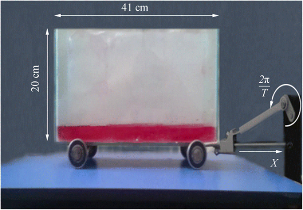Figure  1  Experimental setup comprising the tank and crank-and-slider mechanism

Download: Full-Size Img

First, the crank and the slider were connected to the engine; then, the glass box was set on a cart (four wheels), and the cart was attached to the crank. The engine was set to a certain revolution per minute (rpm). The glass box was filled with water to a height of 2.5 cm. A charge-coupled device camera with 21 megapixels was used to record the video films. To extract the images from these video films at a certain time, the Video Image Master Pro application was used. In these experiments, the tank motion was defined as follows:

The glass tank featured horizontal oscillation with a fixed period (T = 1 s) and domain (A = 0.045 m). Owing to the low speed of the tank movement, no modulation or ramping was considered. In each case, the laboratory model was first ran, and the process was simultaneously filmed by the camera above the tank. The images were then extracted at different times by Video Image Master Pro; the results were comparable with the numerical solution results.

For the numerical simulation, the grid was examined under four different node numbers (n = 480000, 956000, 1435000, and 1920000). The free surface profiles for these four cases are shown in Figure 2.

Figure  2  Grid study: the effect of mesh number on free surface variations at t = 2.1 s

Download: Full-Size Img

As shown in Figure 2, as the number of particles increased, the difference between the free surface profiles decreased, indicating convergence. Therefore, the grid with 1 435 000 nodes was selected for the numerical simulations.

The free surface variations are displayed in Figure 3.

Figure  3  Comparison between model predictions and experimental results for t = 3.35 s

Download: Full-Size Img

The structure motion is transferred to the water, which leads to a right–left oscillating fluid motion. Continuous fluid flow occurs along the horizontal surface until the liquid fluid reaches the vertical wall. Then, the liquid moves upward along the right side of the vertical wall. The liquid then returns and accumulates. In this condition, a violent flow was observed in all the cases shown in Figure 3. This flow was frequently repeated and created collapses of water on the vertical walls. This violent flow created high-amplitude forces with high wave heights. If the wave height is controlled, the force domain will also be controlled.

For CFD modeling of the sloshing phenomenon, in Figure 3, the modeling results of this flow by eight turbulence models are shown. All the models except the standard k–ε model agreed well with the experimental results. One of the most challenging problems in the modeling of this phenomenon is selecting a suitable turbulence model. Therefore, eight different turbulence models were examined in this study.

Figures 3, 4, 5, 6, 7, and 8 show the experimental results and model predictions (different turbulence models) for t = 3.45 s, t = 3.85 s, and t = 4.15 s.

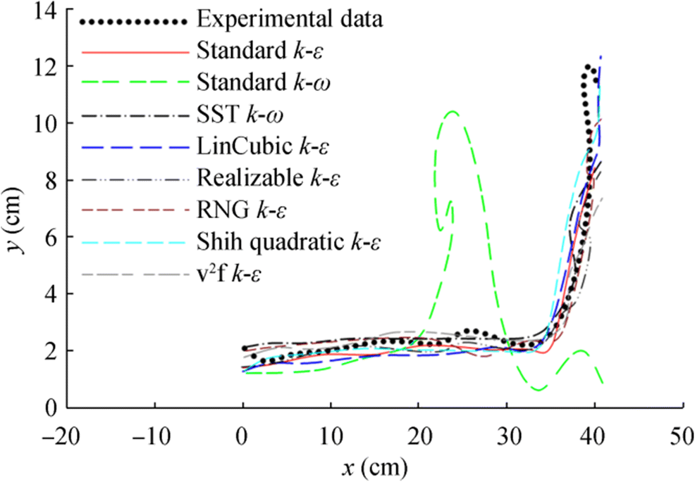Figure  4  Comparison between free surface profiles from numerical models and experimental result for t = 3.35 s

Download: Full-Size Img

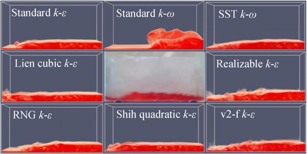Figure  5  Comparison between model predictions and experimental results for t = 3.85 s

Download: Full-Size Img

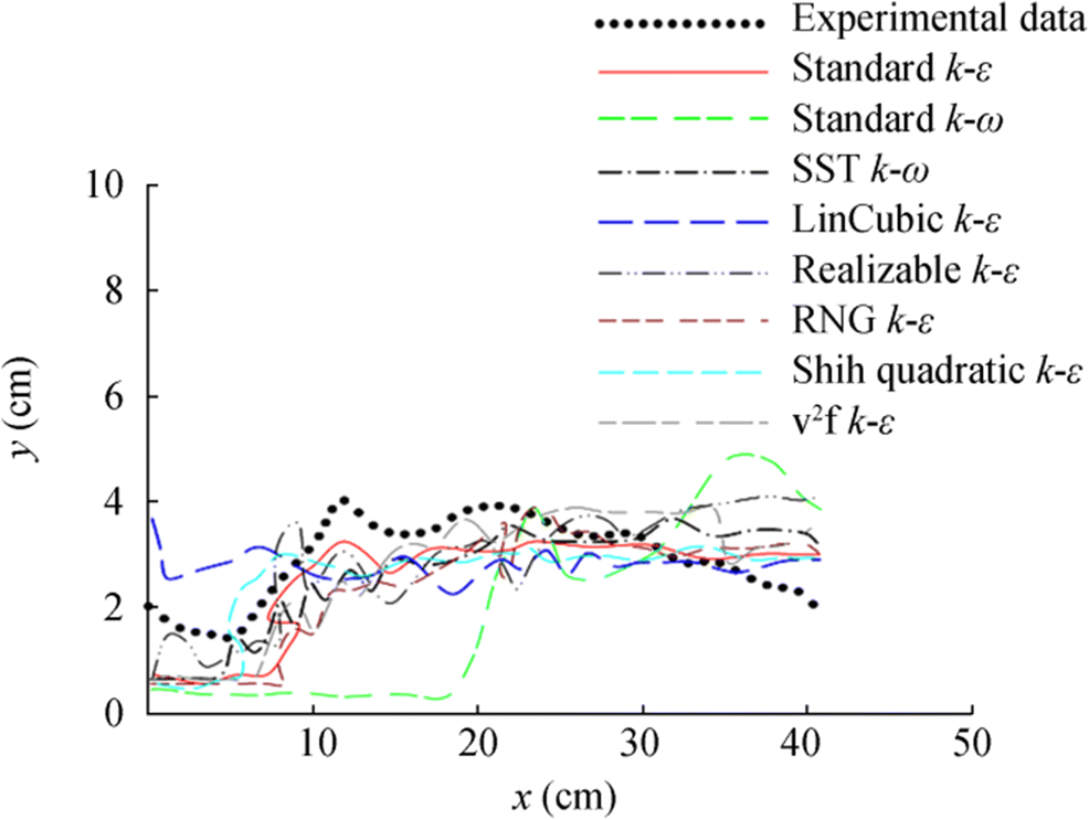Figure  6  Comparison between free surface profiles from numerical models and experimental result for t = 3.85 s

Download: Full-Size Img

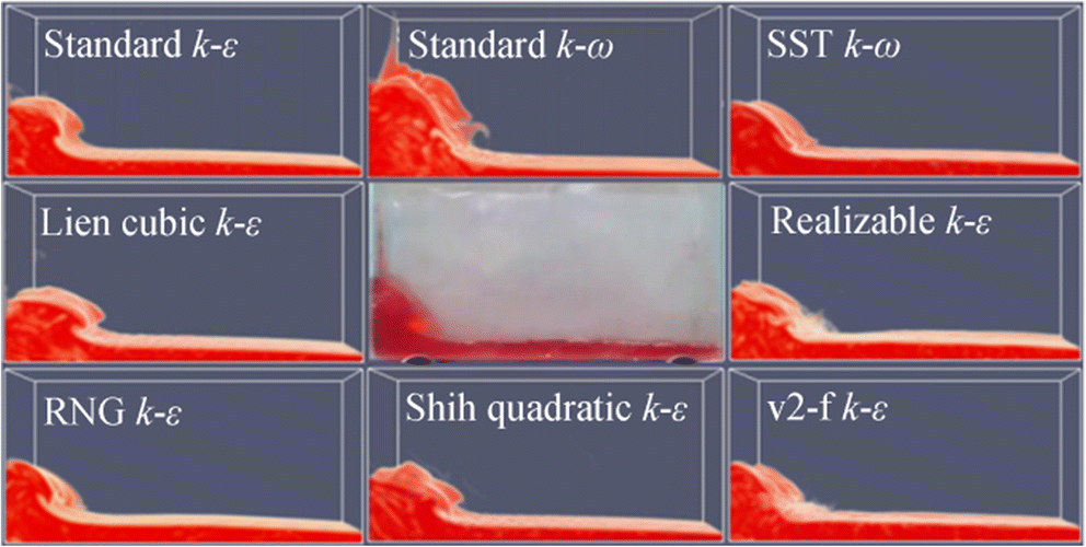Figure  7  Comparison between the model predictions and experimental results for t = 4.15 s

Download: Full-Size Img

Figure  8  Comparison between free surface profiles from numerical models and experimental result for t = 4.15 s

Download: Full-Size Img

For a better comparison, the plots of the free surface profiles obtained from these eight turbulence models are presented in Figures 4, 6, and 8. The standard k–ε model features a remarkable error and thus is not suitable for modeling the sloshing phenomenon. The figure also shows that the k–ε models are more suitable than the k–ω models to model this phenomenon.

Figure 5 shows the fluid motion in the box for t = 3.85 s for all eight turbulence models and compares their predictions with the experimental results.

Figure 7 also shows the variation of the free surface for these eight models for t = 4.15 s.

As also indicated in Figures 5 and 7, the standard k–ε model was the worst method for modeling the sloshing phenomenon. However, the SST k–ε model seems to be a more suitable method than the k–ω method. The SST model predicted the transport of the turbulent shear stress and yielded highly accurate predictions of the onset and the flow separation under adverse pressure gradients. In fact, the SST model was developed to overcome the insufficiencies of the standard k–ε model.

In the Lien cubic k–ε model, the cubic fragments enhance the turbulence level in stagnation regions, which is contrary to the desired response, but qualitatively mimic the sensitivity to streamline curvature in relatively simple flows (Lien et al. 1996). An immediate benefit of the realizable k–ε model is that it is more accurate and consistent for predicting the spreading rate of both planar and round jets. It is also likely to provide higher performance for flows involving rotation, boundary layers under robust adverse pressure gradients, separation, and recirculation. The RNG model has an additional term in its ε equation that significantly improves the accuracy of rapidly strained flows. Moreover, the effect of swirl on turbulence is included in the RNG model, enhancing the accuracy for swirling flows. The RNG theory provides an analytical formula for turbulent Prandtl numbers, while the standard k–ε model uses user-specified constant values. While the standard k–ε model is a high-Reynolds-number model, the RNG theory provides an analytically derived differential formula for effective viscosity that accounts for low-Reynolds-number effects. The effective use of this feature, however, depends on the appropriate treatment of the near-wall region. The Shih k–ε model has been categorized among nonlinear eddy viscosity models. The nonlinear eddy viscosity models algebraically link the turbulent stresses to the strain rate and contain higher-order quadratic and cubic terms. They often give improved predictions in reattachment areas where the linear models sometimes fail to correctly predict the flow (Shih et al. 1995).

An instant benefit of the realizable k-ε model is that it offers improved estimations for the spreading rate of both planar and round jets. It also shows superior performance for flows involving rotation, boundary layers under strong adverse pressure gradients, separation, and recirculation. In nearly every measure of comparison, the realizable k–ε model demonstrates a superior ability to capture the mean flow of complex structures. The v2-f k–ε model is categorized among the RANS models and has been developed to accurately trace turbulence anisotropy near the solid wall; therefore, it provides higher predictions of flow separation, viscous drag, and heat transfer. The v2-f k–ε model is a development of the classical k–ε model and is obtained by including transport equations for quantities representative of Reynolds stress anisotropy induced by wall blockage. Despite the increased difficulty regarding the standard k–ε model, the v2-f model is numerically stable and reproduces important characteristics of the Reynolds stress transport models without introducing computational complications.

Finally, to obtain a proper decision on the best turbulence model for simulating this phenomenon, the mean errors of the presented predictions of each turbulence model in Figures 4, 6, and 8 with respect to the experimental results were calculated and are reported in Table 1. In the table, the turbulence models are ranked by their mean error. To calculate the mean error, the height difference of each point of the liquid free surface in each model case relative to the height of the same point in the experimental case at a given time is calculated; then, the differences at that time are averaged as follows:

where y_i is the height of the ith point on the free surface for each model case, y_{i − exp} is the height of the ith point on the free surface for the experimental case, and N_f is the value of the point considered on the free surface.

As indicated, the RNG k–ε model is the best choice, although the differences between its result and those of the second-best (SST k–ε model) and third-best models (v2-f k-ε) are very small. The standard k–ω model is concluded as the worst choice for modeling the sloshing phenomenon.

The results show that the k–ε models have good treatments. Moreover, the changes imposed in the k–ε model to obtain the RNG model are useful. An analytical formula for the turbulent Prandtl number is introduced for the RNG model, while the standard model is based on user-specific constant values. Also, the RNG model applies an analytically derived differential formula for the effective turbulent viscosity that considers low-Reynolds-number flows; the formula is effective when the near-wall region is appropriately treated. The RNG k–ε model is consequently more accurate and reliable than the standard k–ε model, especially in places where the Reynolds number decreases locally.

To illustrate the effect of pressure on the sliding phenomenon, in Figure 9, the pressure variations within 8 s for the lower-left corner are displayed.

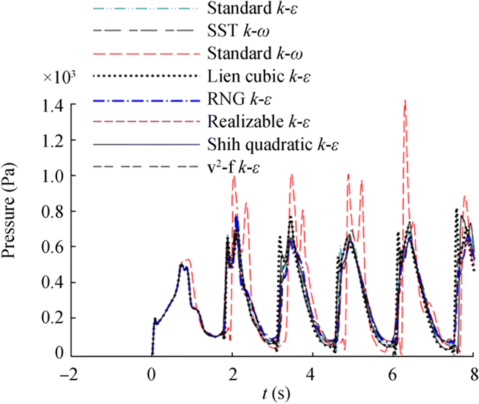Figure  9  Pressure variation with time for the lower-left corner for different turbulence models

Download: Full-Size Img

As shown in the figure, the pressure variations were periodical. The pressure variation curves for most cases are close together, with only the k–ε model exhibiting a significant difference.

4   Conclusion

In the present study, a VOF analysis using OpenFOAM was performed to simulate shallow water sloshing in a rectangular tank. A mechanical mechanism experimental setup was also constructed to record the shallow water sloshing details. The accuracies of the presented algorithms to model the sloshing phenomenon were determined by comparing the numerical and experimental results. The main aim of the study was to investigate the abilities of different turbulence models for simulating the water sloshing phenomenon. The free surface profiles obtained from eight different turbulence models were compared with the recorded experimental results, at three different times. The turbulence models were ranked by their mean error in predicting the free surface behaviors. The RNG k–ε and the standard k–ω models were found to be the best and worst turbulence models for modeling the sloshing phenomenon, respectively; moreover, the SST k–ε model and v2-f k-ε results were very close to the RNG k–ε model result.