1   Introduction

In the Lagrangian meshless/particle methods, for example, the smoothed particle hydrodynamics (SPH, e.g. Monaghan 1994; Shao and Lo 2003; Shao et al. 2006; Khayyer et al. 2008; Lind et al. 2012), moving particle semi-implicit method (MPS, e.g. Koshizuka and Oka 1996; Gotoh and Khayyer 2016; Khayyer and Gotoh 2010), the meshless local Petrov-Galerkin method (MLPG, e.g., Ma 2005a, b; Zhou and Ma 2010), interpolating element-free Galerkin method (Abbaszadeh and Dehghan 2019; Dehghan and Abbaszadeh 2018, 2019), the computational domain is represented by particles and the governing equations with associated boundary conditions are discretised to form a linear algebraic equation system, which leads to the approximation of physical quantities at particle locations. These methods become more popular, attributing to their superiority over the conventional mesh-based methods, such as the finite element method and finite volume method, in dealing with various engineering problems with large deformations, such as the breaking wave impact on offshore structures, for which the mesh-based methods may suffer from significant mesh distortions and/or numerical diffusions.

One key technique for the Lagrangian meshless methods is to numerically formulate and discretise the Laplacian operator, which is required mainly for three purposes. The first one is to discretise the governing equations, involving second-order partial differential terms or Laplacian operators, e.g. the partial differential equation for the heat conduction and thermal diffusion (Chen et al. 1999; Schwaiger 2008), the pressure Poisson's equation employed by the projection-based/fractional step methods for solving the Navier-Stokes (NS) equations to deal with fluid-structure interaction problems (Shao and Lo 2003; Ma et al. 2016) and the Helmholtz equation widely used in wave and diffusion problems. The second one is to numerically estimate specific physical quantities, which are expressed by the Laplacian of others, e.g., the viscous stress in the NS equation (Zheng et al. 2018). The third one is to discretise the Laplacian utilised as stabilisation operators to enhance the pressure calculation in various applications (Khayyer and Gotoh 2010; Khayyer and Gotoh 2012; Ikari et al. 2015). In meshless methods, the Laplacian of a function at a specific location is numerically formulated in terms of discretised function values at surrounding particles within the support domain using finite difference, kernel integration, moving least squares (MLS) or weighted least squares (WLS) algorithms. Therefore, the accuracy, convergence and computational efficiency of the schemes are significantly influenced by the particle distribution. In Eulerian meshless methods for steady problems (e.g., Lind and Stansby 2016), the particles are fixed and may be placed uniformly and regularly. For such problems, high-order finite difference schemes based on a uniform particle distribution can be directly applied to formulate the Laplacian operator. However, in the Lagrangian meshless methods for unsteady problems, the particles move at the material velocity and, consequently, their distribution may be highly disordered even though they may be placed regularly and uniformly in the initial state. Such disorderliness/randomness of the particle distribution considerably downgrades the schemes based on a uniform particle distribution.

For a random/disordered particle distribution, efforts have been devoted to the reviews of various schemes, e.g. on dealing with the viscous term in SPH (Zheng et al. 2018) and on solving pressure Poisson's equation (PPE) involved in projection-based meshless methods (Ma et al. 2016). It has been observed that some schemes (classified as type 1 by Ma et al. 2016), e.g. Cummins and Rudman (1999); Lo and Shao (2002); Lee et al. (2008); Xu et al. (2009); Hu and Adams (2007); Gotoh et al. (2014); and Khayyer and Gotoh (2010, 2012), converge at a rate less than first order for estimating the Laplacian of a given function, although they do not need inversions of any matrices and thus have relatively low computational costs. Their performances may be improved by reducing the randomness of the particle distribution, e.g., using the particle shifting scheme proposed by Lind et al. (2012), or by introducing error correction and compensating terms, e.g. Oger et al. (2007) and Ikari et al. (2015), which requires the inversion of matrices. Alternatively, high-order Laplacian discretisation schemes have also been developed for a random/distorted particle distribution. These include the CSPM proposed by Chen et al. (1999), a scheme proposed by Fatehi and Manzari (2011), which was developed from the Brookshaw's scheme (Brookshaw 1985) by introducing an error compensation, the LSMPS developed by Tamai and Koshizuka (2014) using the MLS algorithm, and LP-MPS proposed by Tamai et al. (2017) using the WLS algorithm. These schemes are classified as type 3 schemes by Ma et al. (2016). Patch tests by Schwaiger (2008), Zheng et al. (2014) and Tamai et al. (2017) have shown that the CSPM, LP-MPS and quadric LSMPS have a higher convergent rate, compared with the type 1 schemes. However, formulating these schemes requires a significant computational cost on inversing matrices at all particle locations and at every time step of the transient simulations. For each particle in 3D problems, the CSPM and LP-MPS need to inverse two matrices with sizes of 6 × 6 and 3 × 3, respectively; the quadric LSMPS needs to inverse a matrix with a size of 10 × 10. To overcome this problem, Schwaiger (2008) proposed a CSPH scheme, which is based on the CSPM but reduces the sizes of inversed matrices to two 3 × 3 for 3D problems, through ignoring the cross-derivative terms of the 2nd derivatives (thus downgrading the accuracy).

In this paper, a quadric semi-analytical finite-difference interpolation scheme (referred to as QSFDI) for numerically formulating the Laplacian operator is developed based on the principle of the linear SFDI (Ma 2008). Its consistency, accuracy and convergence property are similar to the quadric LSMPS and LP-MPS, for randomly distributed particles, whereas the sizes of the matrices to be inversed are considerably reduced to 3 × 3 for 3D problems, compared with 6 × 6 in the quadric LSMPS and LP-MPS. The performance of the present scheme will be assessed by systematic patch tests considering both directly estimating the Laplacian of specific functions and solving Poisson's equation.

2   Mathematical Formulation

Ma (2008) and Ma et al. (2016) developed the linear SFDI, which was based on Taylor's expansion with a leading truncation term of 2nd derivatives, for numerical interpolations and gradient estimations. The patch test by Ma (2008) suggested that the linear SFDI is superior over the linear MLS when the particles are randomly distributed. The principle of the SFDI is extended here to derive the interpolation, gradient estimation and Laplacian discretisation schemes with a quadric accuracy.

For each particle j at x_j, which locates inside the support domain of Point x_I, a function p can be expressed as Taylor's expansion,

where x = [x y z]^T, $ {\boldsymbol{r}}_{jI}={\boldsymbol{x}}_j-{\boldsymbol{x}}_I={\left[{x}_{jI}\kern0.5em {y}_{jI}\kern0.5em {z}_{jI}\right]}^{\mathrm{T}} $ and ∇ is the spatial differential operator. In Eq. (1), the 2nd derivative term $ \frac{1}{2}{\left({\boldsymbol{r}}_{jI}^T\nabla \right)}^2p\left(\boldsymbol{x}\right) $ in the conventional Taylor's expansion (e.g. Chen et al. 1999; Tamai et al. 2017) is split into two, i.e. $ \frac{1}{2}{\left({\boldsymbol{r}}_{jI}^{(2s)}\right)}^{\mathrm{T}}{{\bf{\nabla}}}^{(2s)}p\left(\boldsymbol{x}\right) $ and $ {\left({\boldsymbol{r}}_{jI}^{(2c)}\right)}^{\mathrm{T}}{{\bf{\nabla}}}^{(2c)}p\left(\boldsymbol{x}\right) $ where $ {\boldsymbol{r}}_{jI}^{(2s)}={\left[{x}_{jI}^2\kern0.5em {y}_{jI}^2\kern0.5em {z}_{jI}^2\right]}^{\mathrm{T}} $, $ {\boldsymbol{r}}_{jI}^{(2c)}={\left[{x}_{jI}{y}_{jI}\kern0.5em {x}_{jI}{z}_{jI}\kern0.5em {y}_{jI}{z}_{jI}\right]}^{\mathrm{T}} $, $ {{\bf{\nabla}}}^{(2s)}={\left[\frac{\partial^2}{\partial {x}^2}\kern0.5em \frac{\partial^2}{\partial {y}^2}\kern0.5em \frac{\partial^2}{\partial {z}^2}\right]}^{\mathrm{T}} $, and $ {{\bf{\nabla}}}^{(2c)}={\left[\frac{\partial^2}{\partial x\partial y}\kern0.5em \frac{\partial^2}{\partial x\partial z}\kern0.5em \frac{\partial^2}{\partial y\partial z}\right]}^{\mathrm{T}} $. Following Ma (2008), the weighted summation of Eq. (1) for all particles in the support domain of Point x_I are used to derive the schemes for approximating the gradient ∇p(x), 2nd derivatives and Laplacian ∇²p(x), as well as the interpolation function for approximating p(x) at x_I. The details of the derivation are presented in Appendix 1. Only the final formulas are summarised below:

where 〈〉 indicates an approximated value; $ \boldsymbol{I}={\left[1\kern0.5em 1\kern0.5em 1\right]}^{\mathrm{T}} $; w_jI is the weighting function for particle j related to x_I; d_jI is the distance between particle j and x_I; definitions of matrices M_{2c, I}, M_{2s, I}, M_{1q, I}, q_jI, Γ_jI, Π_jI and G_jI can be found in Appendix 1. In practices, Eq. (3) can be applied to discretising the Poisson's equation at all particle positions and/or to directly estimating ∇²p(x) at point x_I coinciding with a particle location. However, if x_I does not coincide with any particles, the value p_I needs to be numerically interpolated in order to estimate $ {{{\bf{\nabla}}}^{\bf{2}}p\left(\boldsymbol{x}\right)}|_{\boldsymbol{x}={\boldsymbol{x}}_I} $. For this purpose, the interpolation function in the QSFDI is also derived and formulated in Appendix 1. Replacing p_I in Eq. (3) by its approximated value 〈p_I〉 using Eq. (33), it leads to

for approximating the Laplacian at a position that does not coincide with particles. The leading truncation errors for Eqs. (2) and (3) are

and

respectively, where $ {\nabla}^{(3)}={\left[\frac{\partial^3}{\partial {x}^3}\kern0.5em \frac{\partial^3}{\partial {x}^2\partial y}\kern0.5em \frac{\partial^3}{\partial {x}^2\partial z}\kern0.5em \frac{\partial^3}{\partial x\partial {y}^2}\kern0.5em \frac{\partial^3}{\partial x\partial y\partial z}\kern0.5em \frac{\partial^3}{\partial x\partial {z}^2}\kern0.5em \frac{\partial^3}{\partial {y}^3}\kern0.5em \frac{\partial^3}{\partial {y}^2\partial z}\kern0.5em \frac{\partial^3}{\partial y\partial {z}^2}\kern0.5em \frac{\partial^3}{\partial {z}^3}\right]}^{\mathrm{T}} $ and the definition of matrix F_jI can be found in Appendix 1. For a random/disordered particle distribution, the leading truncation errors corresponding to the gradient estimation (Eq. (5)), the Laplacian discretisation (Eq. (6)) and the numerical interpolation to approximate 〈p_I〉 (Eq. (34)) are all proportional to $ {{{\bf{\nabla}}}^{(3)}p\left(\boldsymbol{x}\right)}|_{\boldsymbol{x}={\boldsymbol{x}}_I}. $ This implies that the QSFDI leads to the exact solution for quadric polynomials for the numerical interpolation, gradient estimation and Laplacian discretisation. The consistency of the QSFDI is the same as the LP-MPS developed by Tamai et al. (2017) and the quadric LSMPS (Quinlan et al. 2006). However, the error analysis on the CSPM (Chen et al. 1999) and Schwaiger's scheme (Schwaiger 2008) given in Appendix 2 suggests that their leading truncation errors is proportional to $ {{{\bf{\nabla}}}^{(2)}p\left(\boldsymbol{x}\right)}|_{\boldsymbol{x}={\boldsymbol{x}}_I} $ for the cases with a random/disordered particle distribution. The consistency of these schemes is one-order lower than the QSFDI. It is worth noting that ∇⁽²⁾p(x) in the leading truncation error of the CSPM, i.e. Eq. (42), origins from the leading truncation error of the gradient approximation scheme proposed in the CSPM, i.e. Eq. (40). This approximation can be replaced by a higher-order gradient estimation scheme, e.g. Eq. (48), to improve the accuracy and the consistency of the Laplacian discretisation, as demonstrated in Appendix 2. The formulation based on Eq. (48) is referred to as the ICSPM in the rest of the paper and summarised below,

where m_j/ρ_j is the volume (area) represented by particle j; and $ {\boldsymbol{I}}_{\mathrm{CSPM}}={\left[\begin{array}{cc}1& 0\end{array}\kern0.5em \begin{array}{cc}0& 1\end{array}\kern0.5em \begin{array}{cc}0& 1\end{array}\right]}^{\mathrm{T}} $; the definitions of matrices M_{2, ICSPM}, M_{2, CSPM} and M_{1, CSPM} are given in Appendix 2. The leading truncation error of Eq. (7) is

which is proportional to $ {{{\bf{\nabla}}}^{(3)}p\left(\boldsymbol{x}\right)}|_{\boldsymbol{x}={\boldsymbol{x}}_I}, $ the same as the quadric LSMPS, LP-MPS and the present QSFDI. It shall be noted that the leading truncation errors of the schemes discussed above are not only dominated by the terms of high-order derivatives (e.g. ∇⁽³⁾p(x) for the QSFDI and ICSPM), which may reflect the accuracy level and the consistency, but also subjected to the corresponding orders of magnitudes, which indicates the convergence rates and are influenced by the mean particle spacing, s₀, the weighting/kernel function, the radius of the support domain and the randomness of the particle distributions. One may follow Quinlan et al. (2006) and Fatehi and Manzari (2011) to carry out a further theoretical analysis on the orders of magnitude of the truncation error; however, patch tests will be used in this paper to demonstrate the convergence properties of the QSFDI and the ICSMP.

Compared with the leading truncation error, it is equally important to look at the number and sizes of the matrices to be inversed in order to formulate the Laplacian operator. For the QSFDI, to approximate the gradient, the 2nd derivatives and the Laplacian of p(x), three matrices, i.e. M_{2c, I}, M_{2s, I} and M_{1q, I}, need to be inversed. For 3D problems, they all have sizes of 3 × 3, whereas for 2D problems, the sizes of M_{2s, I} and M_{1q, I} are 2 × 2 and M_{2c, I} is a scalar. The sizes of matrices to be inversed for formulating the Laplacian in the QSFDI are slightly higher than the Schwaiger's scheme (e.g. CSPH2Γ) for 3D problems but considerably lower than the LP-MPS, the quadric LSMPS and the CSPM, for which the number and the sizes of matrices to be inversed are summarised in Table 1. As mentioned above, an improved scheme for CSPM, i.e., ICSPM is also introduced. The number and sizes of the matrices to be inversed in the ICSPM are the same as the original CSPM, although the accuracy of the former is one order higher than the latter for a random particle distribution.

It is well known that the CPU time spent on the inversion of a matrix with size of M × M with M being 2 to 10 is proportional to M³. The CPU time spent on matrix inversions for 2D problems may be indicated by ~ 2 × 2³ for CSPH2Γ and QSFDI, ~ 2³ + 3³ for CSPM, LP-MPS and ICSPM, ~ 6³ for quadric LSMPS. The CPU time by the QSFDI on matrix inversions is approximately 45.7% of those by the LP-MPS or ICSPM, and 7.4% of that by the quadric LSMPS for 2D problems. The corresponding figures for 3D problems are 40% and 8.1%, respectively. Nevertheless, different schemes require different CPU time on formulating the matrices; the overall robustness of these schemes will be investigated in the following patch tests.

3   Patch Test

To quantify the accuracy, convergence and robustness of the QSFDI and ICSPM, patch tests are performed using various cases. As indicated above, some of the main purposes for the Laplacian discretisation are (1) to find physical quantities, which may be expressed as the Laplacian of others, and (2) to discretise the Poisson's equations. For the former, the Laplacians of various specified functions f(x, y), which are frequently used in literatures are directly estimated. For the latter, the Poisson's equation are considered:

where the function denoted by (R. H. S) is pre-specified as the real values of the Laplacian of f(x, y). The present QSFDI, ICSPM and other existing schemes listed in Table 1 are employed for comparisons in the patch tests. When the ICSPM, CSPM and CSPH2Γ are performed, m_j/ρ_j in their formulations is evaluated by using $ 1/\sum \limits_{j=1}^N{W}_{jI} $ (Hu and Adams 2007). It is well known that the kernel/weighting functions play an important role in the convergence and accuracy of the numerical schemes in the meshless method (Quinlan et al. 2006), as demonstrated by the error analysis, e.g. Eqs. (5) and (6), which contains the weighting functions. The main aim of this paper is to introduce the QSFDI and ICSPM, and a quintic spline kernel function (Schwaiger 2008),

where r = d_jI is used as the kernel function of ICSPM, CSPM and CSPH2Γ, and the weighting function of other schemes. By using Eq. (9), the radius of the support domain is 3h. The effect of the kernel/weighting functions will not be investigated and discussed in the future.

3.1   Estimating Laplacian of Specified Functions

Following Schwaiger (2008), the first group of the test functions used is

The computational domain is a unit square with 2 ≤ x ≤3 and 2 ≤ y ≤ 3. The particles are initially generated using a uniform spacing, i.e. ∆x = ∆y = s₀. To reflect the randomness of the particle distribution, a random shift with ∆x^′ = Kδs₀ and ∆y^′ = Kδs₀ is applied to all particles, where K is a scale factor and δ is a random number between − 1 and 1. In the patch tests, K is in the range of 0.1 to 0.8. The Laplacian of the function p at any particle i, 〈∇²p_i〉, are estimated by different schemes summarised in Table 1. The relative error is estimated in the same way as in Schwaiger (2008) for the sake of comparison, given by

where ∇²p_i is the analytical value of the Laplacian of the function p at Particle i; N is the total number of particles at which the Laplacian are estimated. It shall be pointed out that all existing schemes suffer from a downgraded accuracy when being applied to the particles near the boundaries due to the fact that the support domain is not full (Chen et al. 1999; Schwaiger 2008) or the neighbouring particles are mainly distributed in a quadrant or a half of the support domain of the particles. For simplicity, as well as being consistent with Schwaiger (2008), only the inner particles within a region of 2.25 < x < 2.75 and 2.25 < y < 2.75 are considered for the error evaluation using Eq. (11). Different s₀ (between 0.1 and 0.00025) and ratio h/s₀ (ranging from 0.75 to 1.2) are considered in the patch test. For specific s₀, h/s₀ and K, at least 10 repeated tests are carried out in order to eliminate the possible abnormality in the random series, the relative error and CPU times are taken as the mean values of the repeated tests.

Figure 1 compares the relative errors for estimating the Laplacian of p(x, y) = x⁶y⁶ using different schemes with a randomness specified by K = 0.4. As can be seen, the LP-MPS, quadric LSMPS and the present QSFDI result in a linear rate of reduction of the relative error as s₀ decreases, while the CSPM and CSPH2Γ do not seem to be convergent as s₀ decreases for a constant ratio of h/s_0, conforming to the patch tests in Schwaiger (2008). Compared with CSPM, the relative error of the ICSPM not only is lower but also reduces linearly as s₀ decreases. It is also observed from Figure 1 that the present QSFDI leads to almost identical results as the LP-MPS, which are more accurate than other schemes, for all values of h/s₀ and s₀ applied in the patch test. As analysed in Section 2, the QSFDI demands less computational efforts on matrix inversions than the LP-MPS; the overall CPU time spent by the former is expected to be shorter than the latter. This is confirmed by Figure 2, which shows that the average CPU time spent by the QSFDI is approximately 20% less than that by the LP-MPS for achieving results with the same accuracy. In addition, Figure 3 displays the relative errors of the Laplacian discretisation against CPU times by different schemes in the cases with K = 0.4 and different values of h/s₀. For convenience, the CPU times are scaled by the reference duration, T_Ref, which is the CPU time spent by the CSPH2Γ with s₀ = 0.1 and h = 0.75s₀. Both Figures 2 and 3 confirm that the QSFDI requires considerably shorter CPU time than all other schemes for achieving a specific accuracy of estimating the Laplacian of function p(x, y) = x⁶y⁶.

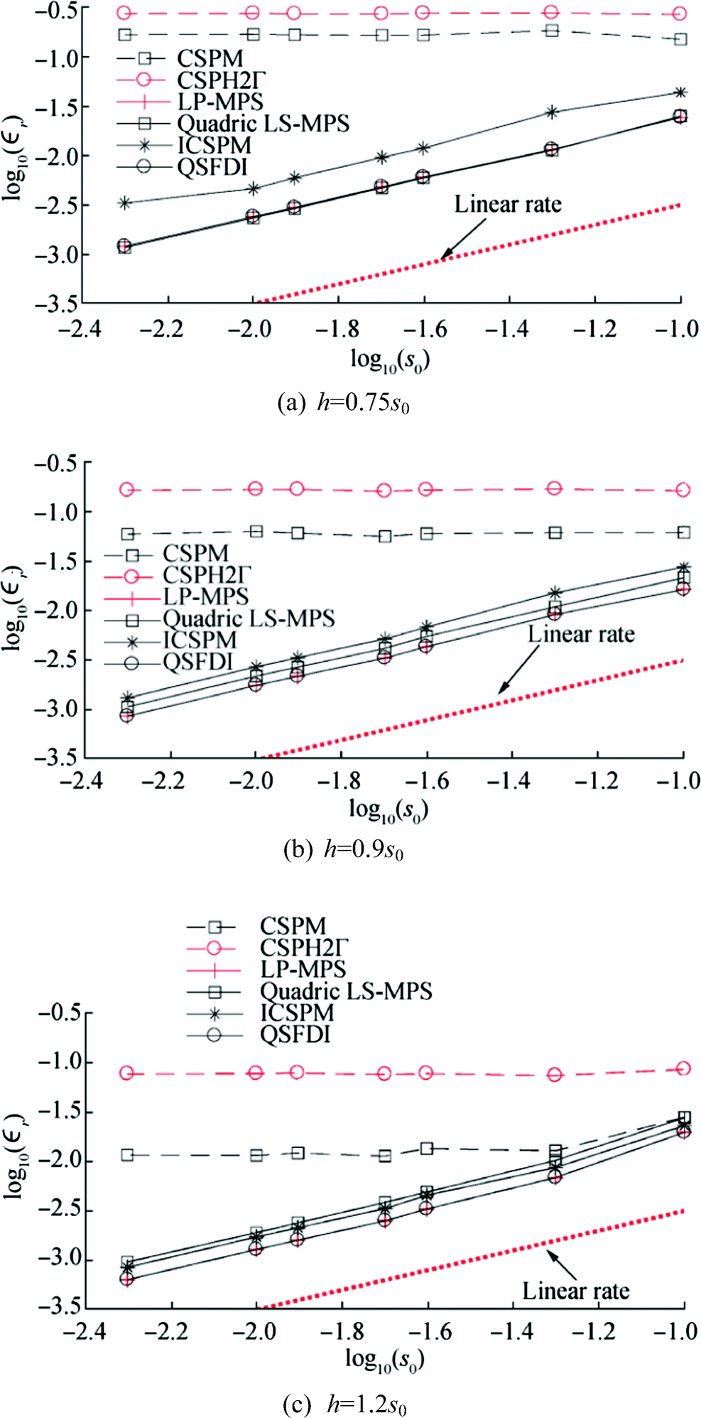Figure  1  Relative error of Laplacian discretisation vs mean particle spacing s₀ for estimating Laplacian of p(x, y) = x⁶y⁶ (K = 0.4; error estimation domain 2.25 < x < 2.75, 2.25 < y < 2.75). a h = 0.75s₀. b h = 0.9s₀. c h = 1.2s₀

Download: Full-Size Img

Figure  2  Ratio of the CPU time spent by the LP-MPS and that by the QSFDI on estimating Laplacian of p(x, y) = x⁶y⁶ (K = 0.4)

Download: Full-Size Img

Figure  3  Relative error of Laplacian discretisation vs CPU time for estimating Laplacian of p(x, y) = x⁶y⁶ (K = 0.4; T_Ref is the CPU time spent by CSPH2Γ with s₀ = 0.1 and h = 0.75s₀; error estimation domain 2.25 < x < 2.75, 2.25 < y < 2.75). a h = 0.75s₀. b h = 0.9s₀. c h = 1.2s₀

Download: Full-Size Img

It shall be pointed out that Schwaiger (2008) and Zheng et al. (2014) have adopted h/s₀ $ =0.268/\sqrt{s_0} $ in the CSPM and CSPH2Γ, based on the error analysis by Quinlan et al. (2006). A linear convergence was observed in their patch tests. By adopting such a strategy, the relative sizes of the support (kernel integration) domain increase as s₀ decreases (e.g. h/s₀ are approximately 0.85 and 2.68 for s₀ = 0.1 and 0.01, respectively). However, as the increase of h/s₀, more neighbouring particles are included in the kernel integration, yielding a considerably increase of CPU time spent on the Laplacian discretisation for each particle. In fact, not only the CSPM and CSPH2Γ, the accuracies and the robustness of all schemes may be significantly influenced by the ratio h/s₀. To further illustrate the effects of the ratio h/s₀ on the robustness of the schemes, an alternative of Figure 3 is presented in Figure 4. For clarity, the corresponding results by the CSPH2Γ, ICSPM and QSFDI are shown in Figure 4a; those by the CSPM, quadric LSMPS and the LP-MPS are shown in Figure 4b. It is observed that the robustness of the QSFDI, LP-MPS and quadric LSMPS is much less sensitive than that of CSPM, CSPH2Γ, and ICSPM to the variation of h/s₀, though the robustness of all the schemes is improved with the increase of h/s₀. It implies that one may optimise the kernel/weighting function and the configuration of the h/s₀ to accelerate the convergent rates for these schemes. Nevertheless, it is not the focus of this paper and, therefore, only constant ratio h/s₀ is considered in the rest of the paper.

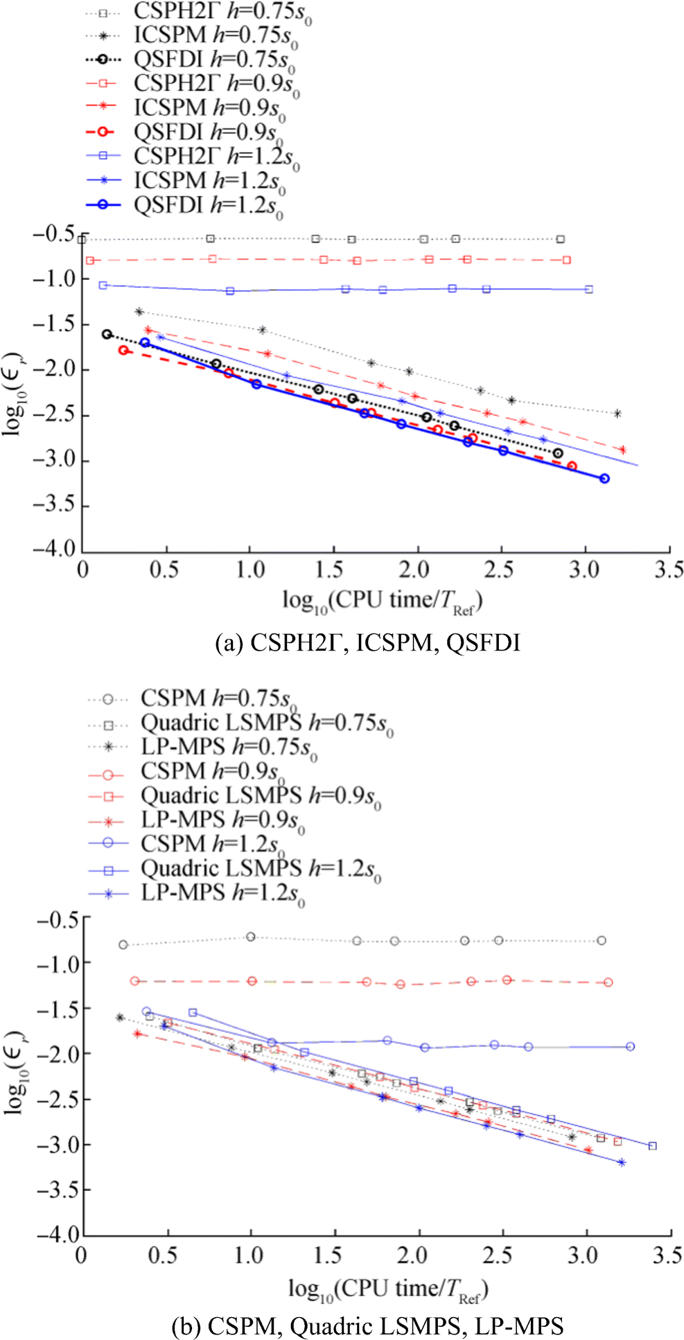Figure  4  Relative error of Laplacian discretisation vs CPU time for estimating Laplacian of p(x, y) = x⁶y⁶ in the cases with different ratios h/s₀ (K = 0.4; T_Ref is the CPU time spent by CSPH2Γ with s₀ = 0.1 and h = 0.75 s₀; error estimation domain 2.25 < x < 2.75, 2.25 < y < 2.75). a CSPH2Γ, ICSPM, QSFDI. b CSPM, Quadric LSMPS, LP-MPS

Download: Full-Size Img

Similar behaviours to Figures 1 and 2 have been observed in the cases with other values of K. Some results are shown in Figures 5 and 6 for demonstration. To save the space, not all the results with different ratios of h/s₀ are presented. In Figure 5, h/s₀ = 1.2 is used by the CSPM, CSPH2Γ and ICSPM; h/s₀ = 0.75 is adopted by others. In such a way, the CSPM, CSPH2Γ, ICSPM and the LSMPS are expected to have the best robustness and the accuracy compared to other values of h/s₀, whereas the results of the QSFDI and the LP-MPS adopting h/s₀ = 0.75 are worse than the corresponding results with a greater h/s₀, as demonstrated by Figure 4. Again, it is clearly seen that the QSFDI and the LP-MPS lead to the highest accuracy and convergence properties compared to others. The comparison of the CPU time spent by the LP-MPS and the QSFDI in Figure 6 again confirms the superiority of the former in terms of saving CPU time for the cases with a different randomness.

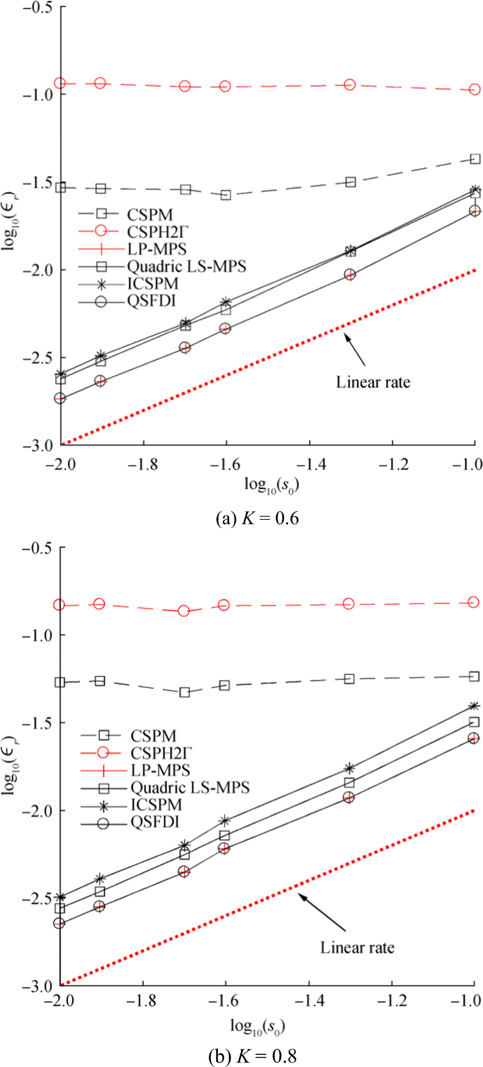Figure  5  Relative error for estimating Laplacian of p(x, y) = x⁶y⁶ for K = 0.6 and K = 0.8 (h = 1.2s₀ for CSPM, CSPH2Γ and ICSPM, h = 0.75s₀ for other schemes; the slopes of the dotted line is 1; error estimation domain 2.25 < x < 2.75, 2.25 < y < 2.75)

Download: Full-Size Img

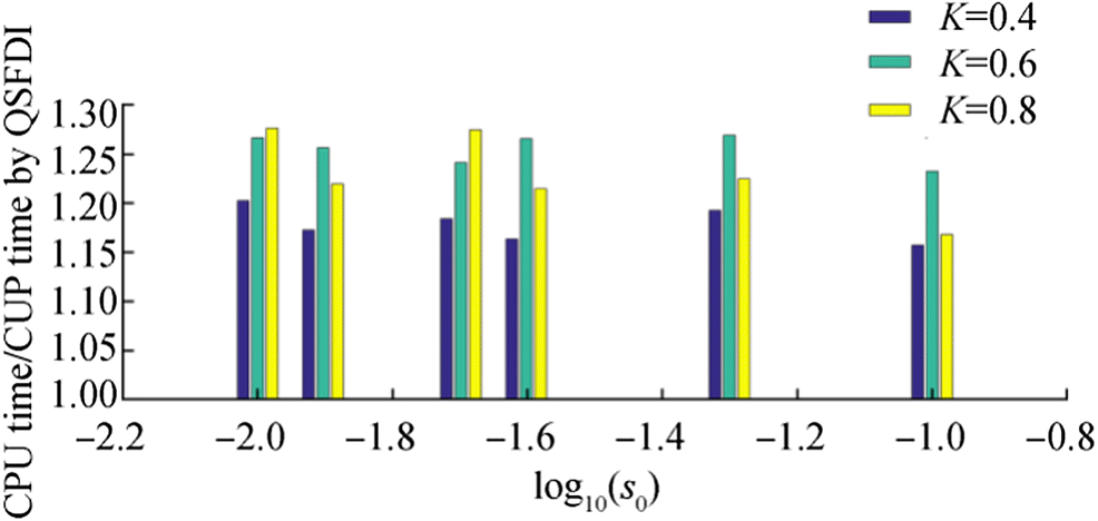Figure  6  Ratio of the CPU time spent by the LP-MPS and that by the QSFDI on estimating Laplacian of p(x, y) = x⁶y⁶ (h = 0.75s₀) for the cases with different randomness of particle distribution

Download: Full-Size Img

Considering the fact that most of analytical formulations used in the engineering problems may be represented by hyperbolic/exponential and/or trigonometric functions (e.g. the velocity potential associated with a linear propagation wave and the temperature in 2D heat conduction problems), the exponential function applied by Tamai et al. (2017)

and a sine function employed by Zheng et al. (2014)

are also considered. In these tests, the computational domain is taken as a unit square with 0 ≤ x ≤ 1; 0 ≤ y ≤ 1. The particle generation is the same as that used in the first test case, i.e. a random distribution with different values of K. The relative error in the tests is defined by

where N is the number of particles for error estimations to be consistent with the references. Similar to the cases shown in Figures 1, 2, and 3, the relative error at inner particles away from boundaries, i.e. 0.25 ≤ x ≤ 0.75; 0.25 ≤ y ≤ 0.75, is assessed. In addition, to reflect the overall performances of different schemes at both the inner particles and boundary particles, the relative error estimated by considering all particles are also assessed.

Figure 7 displays the relative errors for estimating Laplacians of Eqs. (12) and (13) in the cases with K = 0.4. For clarity, the corresponding results by ICSPM are not shown. From Figure 7a, c, in which only inner particles are taken into account when estimating the relative error, it is observed that all schemes converge at a rate between linear and quadric for relatively coarse particle resolutions, i.e. s₀ > 0.01; thereafter, the relative errors of the CSPM and CSPH2Γ seem not to be reduced, whereas the QSFDI, the LP-MPS and quadric LS-MPS converge at a rate slightly higher than a linear rate. As expected, for a specific particle resolution, the relative errors of all the schemes considering all particles (Figure 7b, d) including these on boundaries are relatively higher than the corresponding results considering the inner particles only. The CSPM and CSPH2Γ converge at a rate much lower than a linear rate (the mean slopes of the curves for CSPM and CSPH2Γ are about 1/0.5). The QSFDI, the LP-MPS and quadric LS-MPS converge at a rate with the mean slopes of approximately 1/1.5.

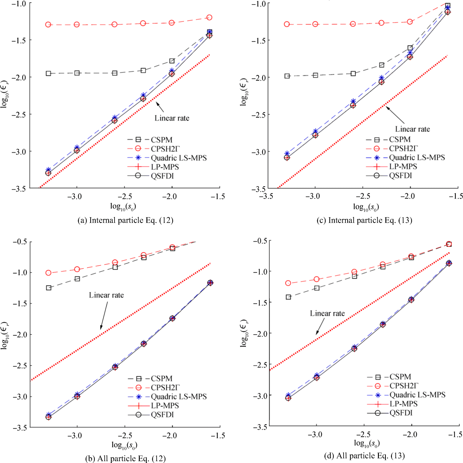Figure  7  Relative error for estimating Laplacians of Eq. (12) and (13) (K = 0.4; h = 1.2s₀ for CSPM and CSPH2Γ, h = 0.9s₀ for other schemes; internal particles located at 2.25 < x < 2.75, 2.25 < y < 2.75 are used for the error estimation in (a) and (c))

Download: Full-Size Img

The same conclusions are achieved in the cases with other randomness, e.g. Figure 8, which displays the relative errors considering all particles for estimating Laplacian of Eqs. (12) and (13), respectively, obtained by using K = 0.8. Examination of the corresponding robustness is also carried out for these cases. The CPU time for different accuracy corresponding to the results of Figure 8 is illustrated in Figure 9. Once again, the superiority of the QSFDI over other schemes in terms of the accuracy and computational costs is clearly observed as in Figures 3 and 6.

Figure  8  Relative error for estimating Laplacians of Eqs. (12) and (13) at all particles (K = 0.8; h = 1.2s₀ for CSPM and CSPH2Γ, h = 0.9s₀ for other schemes

Download: Full-Size Img

Figure  9  CPU times for estimating Laplacians of Eq. (12) and (13) (K = 0.8; h = 1.2s₀ for CSPM and CSPH2Γ, h = 0.9s₀ for other schemes; T_Ref is the CPU time spent by CSPH2Γ with s₀ = 0.1)

Download: Full-Size Img

3.2   Finding solutions of Poisson's equation

Another purpose of the Laplacian discretisation is to discretise the governing equation, e.g. the Poisson's equation, to find its numerical solution. Relevant patch tests presented in this section will use a computational domain of a unit square (0 ≤ x ≤ 1, 0 ≤ y ≤ 1), the same as that for Figures 7, 8, and 9. In this test, the Poisson's equation defined by Eq. (8), of which (R. H. S) are specified by the Laplacians of a given function. The Dirichlet condition on all boundaries of the domain is applied, i.e. p at all boundary particles are specified to be consistent with (R. H. S). Under this condition, the analytical solution of the Poisson's equation (Eq. (8)) in the computational domain is the function p(x, y). For example, if Eq. (13) is applied as the function p(x, y), (R. H. S) = − 100 sin(6x + 8y) and the values on the boundary at x = 1.0 is sin(6 + 8y). The Poisson's equation is discretised at all internal particles by using different schemes to form linear algebraic equations, which is solved by the GMRESS solver, resulting in the solutions of p(x, y) at all internal particles. For the results shown below, the control residual adopted by the GMRESS solver is 10⁻⁴, which is sufficiently small (comparison with the corresponding results obtained using a control residual of 10⁻⁸ shows that the difference is smaller than 0.1%). The relative error of the numerical solution against the analytical solution is evaluated by

where p_i and p_{i, a} are the numerical approximation and the analytical value, respectively, at particle i; N_t is the total number of internal particles.

Figure 10 compares the relative errors of numerical solutions to the Poisson's equations, whose (R. H. S) are given by the Laplacian of Eqs. (12) and (13), respectively, with the moderate randomness of particle distribution (K = 0.4). It is observed that the convergent rates of the LP-MPS, quadric LS-MPS, ICSPM and the QSFDI are quadric for all particle spacing. In contrast, as s₀ decreases, the relative errors of the CSPM and CSPH2Γ reduces at a quadric rate for relatively coarse resolutions (when the error is large); however, it reduces to a linear or lower rate for finer particle resolutions (when the error becomes acceptably small). The comparison of the relative errors for a specific particle spacing indicates that the QSFDI and the LP-MPS result in the most accurate solutions. The corresponding comparisons of the CPU time are illustrated in Figure 11. Unlike the direct Laplacian discretisation presented in Section 3.1, the CPU time spent on achieving the solutions to the Poisson's equation is also influenced by the effectiveness of the linear algebraic solver and its pre-conditioner, i.e. the initial value. By using the solver briefed above, the total CPU time spent by the QSFDI is slightly shorter than the LP-MPS but significantly shorter than all other schemes.

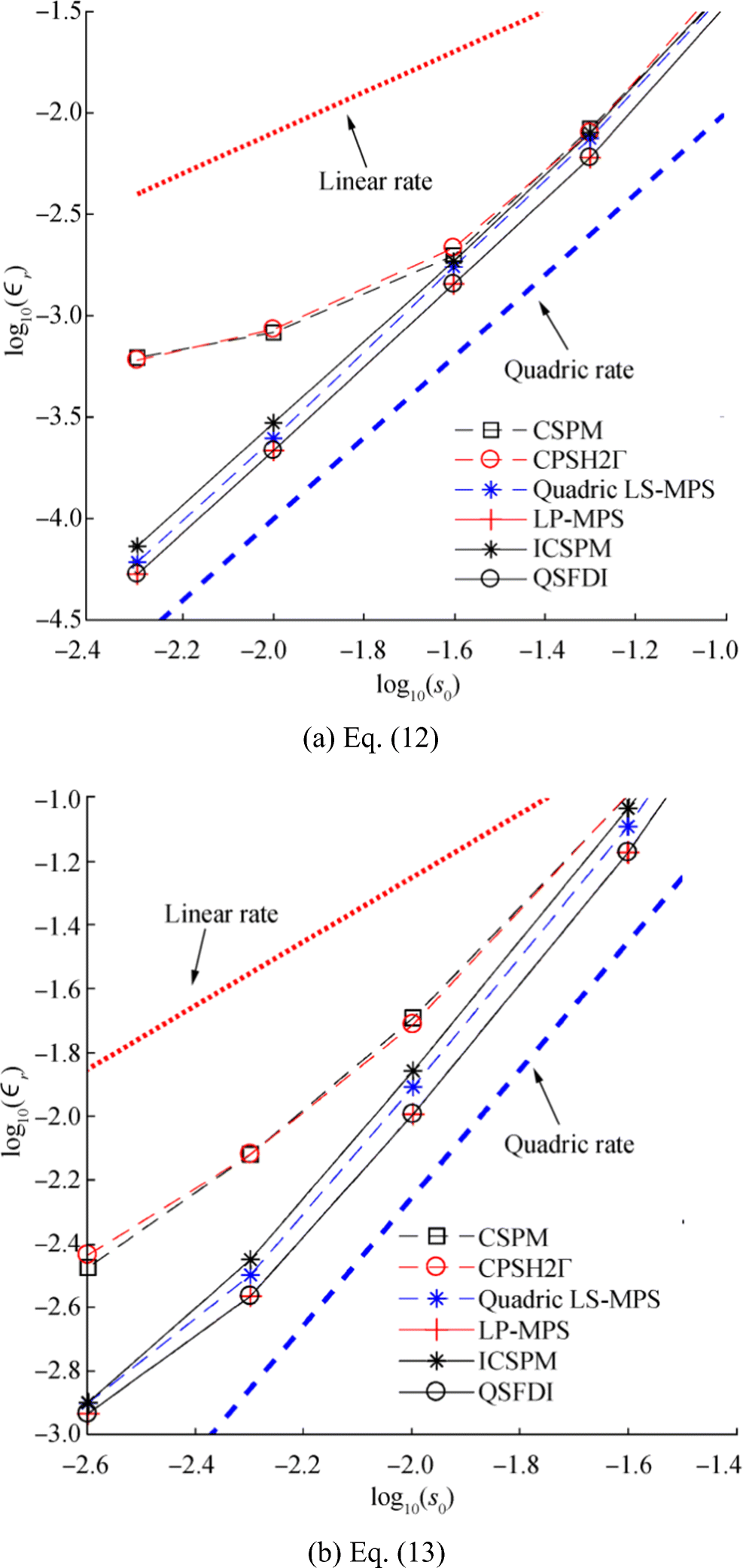Figure  10  Relative error of solution to Poisson's equation based on Eq. (12) and Eq. (13) (K = 0.4, h = 1.2s₀ for CSPM, CSPH2Γ and ICSPM, h = 0.9s₀ for other schemes)

Download: Full-Size Img

Figure  11  CPU times for solving Poisson's equation based on Eqs. (12) and (13) (K = 0.4, h = 1.2s₀ for CSPM, CSPH2Γ and ICSPM, h = 0.9s₀ for other schemes)

Download: Full-Size Img

Different values of K and h are also used in this investigation. Some results are illustrated in Figures 12 and 13 for K = 0.6 and 0.8 respectively, where h = 1.2s₀ are used for all schemes. For clarity, the corresponding results with the quadric LP-MPS and the ICSPM are not shown. As can be seen, with severer randomness of particle distribution, the relative errors of the CSPM and CSPH2Γ reduce at a rate less than the linear rate as s₀ decreases, quite different from what has been seen in Figure 10. In contrast, the accuracy and convergent properties of the QSFDI and LP-MPS seem to be insignificantly affected by increasing the randomness (Figures 12a, c and 13a, c). Figures 12b and d and 13b and d reveal that the CPU time by the present QSFDI is generally shorter than all other schemes for achieving satisfactory results, e.g. relative error smaller than 1%. Following the comparison of the robustness of the QSFDI and the LP-MPS in the previous section on estimating Laplacians, the average ratios of the CPU time spent by the LP-MPS and that by the QSFDI are displayed in Figure 14, where h = 1.2s₀, for finding the solutions to the Poisson's equation based on Eq. (13). It clearly shows that the CPU time spent by the QSFDI is approximately 5%–10% shorter than the LP-MPS, although averagely 20% less CPU time on discretising the Poisson's equation than that by the QSFDI is recorded in the patch tests in Section 3.1.

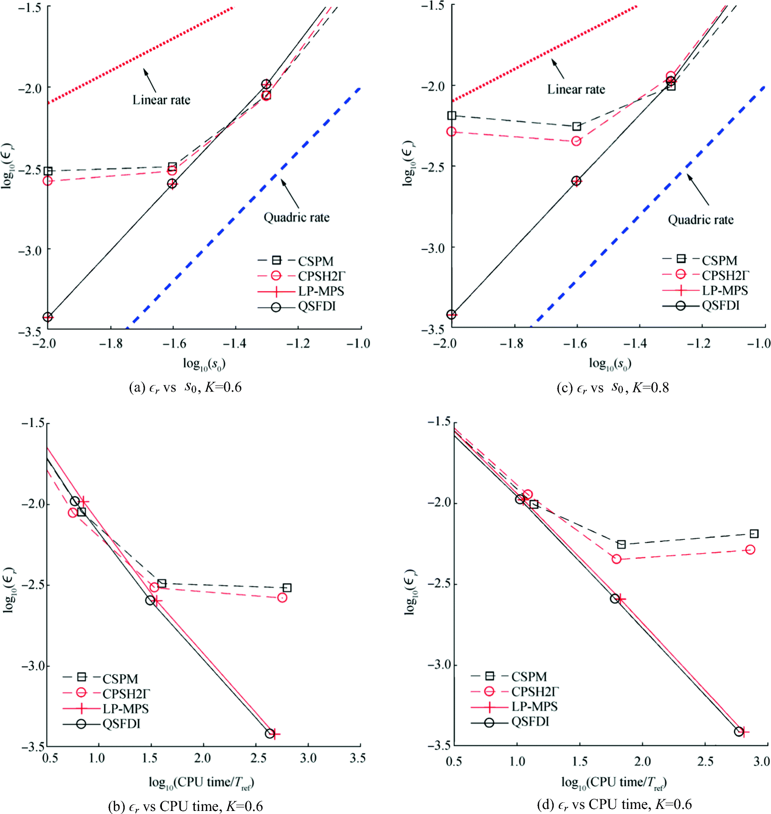Figure  12  Relative error of solution to Poisson's equation based on Eq. (12) and the corresponding CPU time in the cases with different particle randomness (h = 1.2s₀; T_Ref is the CPU time spent by CSPH2Γ with s₀ = 0.1 and K = 0.6)

Download: Full-Size Img

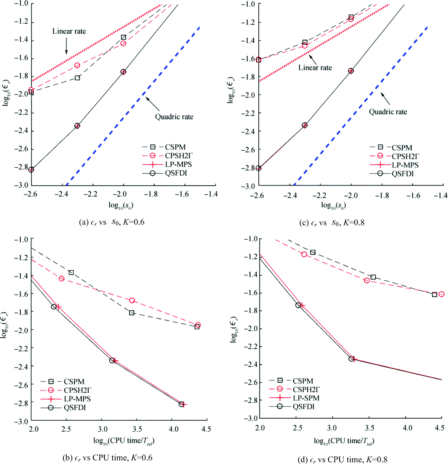Figure  13  Relative error of solution to Poisson's equation based on Eq. (13) and the corresponding CPU time in the cases with increased particle randomness (h = 1.2s₀; T_Ref is the CPU time spent by CSPH2Γ with s₀= 0.1 and K = 0.6)

Download: Full-Size Img

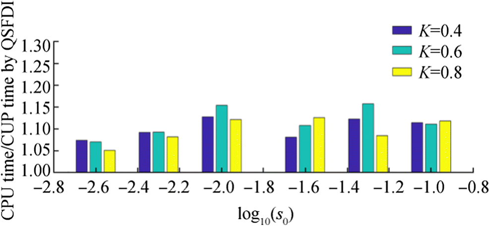Figure  14  Average ratio of the CPU time spent by the LP-MPS against that by the QSFDI in the cases with different randomness for finding solutions to Poisson's equation (h = 1.2s₀)

Download: Full-Size Img

4   Conclusions

This paper develops a new scheme called QSFDI, which adopts the same principle of SFDI, to discretise the Laplacian operator for Lagrangian meshless (particle) methods, in which the particles move during the numerical simulation and exhibit a disordered/random distribution. The accuracy and consistency of the QSFDI are similar to the LSMPS and LP-MPS but higher than the CSPM and CSPH for randomly distributed particles. However, the matrices required to be inversed by the QSFDI have smaller sizes than the LSMPS and LP-MPS. For example, for 3D problems, the size of the matrices to be inversed in the QSFDI is 3 × 3, while it is 6 × 6 in LP-MPS.

Systematic patch tests considering both directly estimating the Laplacian of specific functions and solving Poisson's equations are carried out. In these tests, different functions including polynomials, hyperbolic and trigonometric functions, which may represent typical spatial variations of physical quantities in engineering such as the water waves and the thermodynamics, are considered. The particles used in the patch tests are randomly distributed. It is observed that the QSFDI has the same convergent rate as the LP-MPS and quadric LSMPS, which is higher than that of the CSPM and CSPH in all the cases studied. It is also observed that the QSFDI requires considerably less computational time than all other schemes (such as the LP-MPS) to achieve the same accuracy.

It is worth noting that the QSFDI method presented in the paper does not only give a new formula for the Laplacian discretisation but also provides the new schemes for the numerical interpolation and gradient estimations. This means that one may extend the QSFDI to deal with the first and 2^nd derivatives in differential equations, e.g. the NS equation and advection-diffusion equations, with a linear consistency and quadric accuracy.

It shall be also noted that the implementation of the QSFDI in a Lagrangian meshless method to solve engineering problems, such as wave-structure interaction in maritime engineering, is under study and results will be discussed in other publications.

Appendix 1: Derivation of QSFDI

For each particle j at x_j, which locates inside the support domain Ω_I of point x_I, a function p can be expressed as Taylor's expansion, i.e. Eq. (1). Multiplying Eq. (1) by $ {w}_{jI}{\boldsymbol{r}}_{jI}^{(2c)}/{d}_{jI}^4 $, where w_jI is the weighting function for particle j related to x_I, d_jI is the distance between particle j and x_I, ignoring the truncation error and taking the sum of resultant equations for all particles in Ω_I, it yields

in which $ {\boldsymbol{M}}_{2c,I}={\sum}_{j=1}^N\frac{w_{jI}}{d_{jI}^4}{\boldsymbol{r}}_{jI}^{(2c)}{\left({\boldsymbol{r}}_{jI}^{(2c)}\right)}^{\mathrm{T}} $. For convenience, $ {{\left({\boldsymbol{r}}_{jI}^{\mathrm{T}}{\bf{\nabla}}\right)}^3p\left(\boldsymbol{x}\right)}|_{\boldsymbol{x}={\boldsymbol{x}}_I} $ is re-written as $ {{\left({\boldsymbol{r}}_{jI}^{(3)}\right)}^{\mathrm{T}}{{\bf{\nabla}}}^{(3)}p\left(\boldsymbol{x}\right)}|_{\boldsymbol{x}={\boldsymbol{x}}_I} $, where $ {\boldsymbol{r}}_{jI}^{(3)}= $[$ {x}_{jI}^3 $ $ 3{x}_{jI}^2{y}_{jI} $ $ 3{x}_{jI}^2{z}_{jI} $ $ 3{x}_{jI}{y}_{jI}^2 $ 6x_jIy_jIz_jI $ 3{x}_{jI}{z}_{jI}^2 $ $ {y}_{jI}^3 $ $ 3{y}_{jI}^2{z}_{jI} $ $ 3{y}_{jI}{z}_{jI}^2\kern0.5em {z}_{jI}^3 $]^T, ∇⁽³⁾=[$ \frac{\partial^3}{\partial {x}^3} $ $ \frac{\partial^3}{\partial {x}^2\partial y} $ $ \frac{\partial^3}{\partial {x}^2\partial z} $ $ \frac{\partial^3}{\partial x\partial {y}^2}\kern0.5em \frac{\partial^3}{\partial x\partial y\partial z} $ $ \frac{\partial^3}{\partial x\partial {z}^2} $ $ \frac{\partial^3}{\partial {y}^3} $ $ \frac{\partial^3}{\partial {y}^2\partial z} $ $ \frac{\partial^3}{\partial y\partial {z}^2} $ $ \frac{\partial^3}{\partial {z}^3} $]^T are two 10 × 1 matrices. Substituting Eq. (16) into Eq. (1), it leads to

where

Multiplying Eq. (17) by $ {w}_{jI}{\boldsymbol{\Pi}}_{jI}/{d}_{jI}^4 $ and taking the sum of resultant equations for all particles in Ω_I, it leads to

where

Substituting Eq. (18) to Eq. (17) leads to

Multiplying Eq. (19) by $ {w}_{jI}{\boldsymbol{q}}_{jI}/{d}_{jI}^2 $, where

and taking the sum of resultant equations for all particles in Ω_I, it leads to the formula for approximating the gradient, i.e. $ \left\langle {{\bf{\nabla}}p\left(\boldsymbol{x}\right)}|_{\boldsymbol{x}={\boldsymbol{x}}_I}\right\rangle $, and its leading truncation error, $ {\boldsymbol{E}}_{{{\bf{\nabla}}p\left(\boldsymbol{x}\right)}|_{\boldsymbol{x}={\boldsymbol{x}}_I}} $,

where 〈〉 indicates an approximated value and

Substituting Eq. (20) to Eq. (18), it leads to the formula to approximate the $ {{{\bf{\nabla}}}^{(2s)}p\left(\boldsymbol{x}\right)}|_{\boldsymbol{x}={\boldsymbol{x}}_I} $, i.e.,

with its leading truncation error

The Laplacian can therefore be approximated by using

where $ \boldsymbol{I}={\left[1\kern0.5em 1\kern0.5em 1\right]}^{\mathrm{T}} $. The corresponding leading truncation error is

In practices, Eq. (24) can be applied to discretise the Poisson's equation at all particle positions and/or to directly approximate ∇²p(x) at a point x_I coinciding with a particle location, where p_I is known. However, to estimate ∇²p(x) at a point that does not coincide with any particles, p_I needs to be numerically interpolated using p_j. To do so, estimation of $ {{{\bf{\nabla}}}^{(2c)}p\left(\boldsymbol{x}\right)}|_{\boldsymbol{x}={\boldsymbol{x}}_I} $ in Eq. (1) is required and achieved by substituting Eqs. (20)–(23) to Eq. (15),

with a leading truncation error of

For convenience of deriving the interpolation function, Eqs. (20), (22) and (26) are, respectively, rewritten in a summation form, i.e.

where

Consequently, Eq. (24) can be re-written as

Multiplying Eq. (1) by w_jI /d_jI , taking the sum of resultant equations at all particles in Ω_I , it leads to

Substituting Eqs. (28)–(30) into Eq. (32), the expression for interpolating p _I and its truncation error E _p can be formulated as

where

By replacing p_I in Eq. (10) or Eq. (31), the Laplacian at a point that does not coincide with any particles can be obtained, i.e.

As shown above, the leading truncation errors for numerical interpolation, gradient estimation and Laplacian discretisation in the QSFDI are proportional to the third derivatives $ {{{\bf{\nabla}}}^{(3)}p\left(\boldsymbol{x}\right)}|_{\boldsymbol{x}={\boldsymbol{x}}_I} $, suggesting that the QSFDI provides exact solutions for quadric polynomials.

Appendix 2: Error Analysis of CSPM and improvement

The CSPM is proposed by Chen et al. (1999), which is derived based on the kernel integration of the conventional Taylor's expansion

in which $ {\left({\boldsymbol{r}}_{jI}^{\mathrm{T}}\nabla \right)}^2p\left(\boldsymbol{x}\right) $ and $ {{\left({\boldsymbol{r}}_{jI}^{\mathrm{T}}{\bf{\nabla}}\right)}^3p\left(\boldsymbol{x}\right)}|_{\boldsymbol{x}={\boldsymbol{x}}_I} $ are rewritten as $ {{\left({\boldsymbol{r}}_{jI}^{(2)}\right)}^{\mathrm{T}}{{\bf{\nabla}}}^{(2)}p\left(\boldsymbol{x}\right)}|_{\boldsymbol{x}={\boldsymbol{x}}_I} $ and $ {{\left({\boldsymbol{r}}_{jI}^{(3)}\right)}^{\mathrm{T}}{{\bf{\nabla}}}^{(3)}p\left(\boldsymbol{x}\right)}|_{\boldsymbol{x}={\boldsymbol{x}}_I} $, respectively, and

Multiplying Eq. (36) by ∇⁽²⁾W_jI, where W_jI is the kernel function, and integrating over the support domain Ω_I, yields,

where the kernel integration has been written in a summation from Chen et al. (1999) and m_j/ρ_j is the volume (area) represented by particle j. By ignoring the last two terms in the right-hand side of Eq. (37), the 2nd derivative term $ {{{\bf{\nabla}}}^{(2)}p\left(\boldsymbol{x}\right)}|_{\boldsymbol{x}={\boldsymbol{x}}_I} $ can be approximated by using

where $ {\boldsymbol{M}}_{2,\mathrm{CSPM}}=\sum \limits_{j=1}^N\frac{{{\bf{\nabla}}}^{(2)}{W}_{jI}{m}_j}{\rho_j}{\left({\boldsymbol{r}}_{jI}^{(2)}\right)}^{\mathrm{T}} $, is a matrix with size of 6 × 6 for 3D problems or 3 × 3 for 2D problems. In numerical practices, $ {\nabla p\left(\boldsymbol{x}\right)}|_{\boldsymbol{x}={\boldsymbol{x}}_I} $ is often unavailable and therefore needs to be numerically estimated. To do so, one may multiply Eq. (36) by ∇W_jI and integrate the resultant equation over Ω_I

Chen et al. (1999) ignored the last three terms in the right-hand side of Eq. (39), yielding the scheme for gradient estimation

in which $ {\boldsymbol{M}}_{1,\mathrm{CSPM}}=\sum \limits_{j=1}^N\frac{\nabla {W}_{jI}{m}_j}{\rho_j}{\boldsymbol{r}}_{jI}^{\mathrm{T}} $, is a 3 × 3 matrix for 3D problems or 2 × 2 matrix for 2D problems. The truncation error of Eq. (40) can be expressed by

Replacing ∇p(x) in Eq. (38) by $ \left\langle {\nabla p\left(\boldsymbol{x}\right)}|_{\boldsymbol{x}={\boldsymbol{x}}_I}\right\rangle $ specified by Eq. (40), the following equation in the CSPM to discretise the Laplacian can be achieved

where $ {I}_{\mathrm{CSPM}}={\left[\begin{array}{cc}1& 0\end{array}\kern0.5em \begin{array}{cc}0& 1\end{array}\kern0.5em \begin{array}{cc}0& 1\end{array}\right]}^{\mathrm{T}} $. The truncation error of Eq. (41) is

In the cases with a regular particle distribution and a uniform spacing, $ \sum \limits_{j=1}^N\frac{{{\bf{\nabla}}}^{(2)}{W}_{jI}{m}_j}{\rho_j}{\boldsymbol{r}}_{jI}^{\mathrm{T}}=0 $ and $ \sum \limits_{j=1}^N\frac{{{\bf{\nabla}}}^{(2)}{W}_{jI}{m}_j}{\rho_j}{\left({\boldsymbol{r}}_{jI}^{(3)}\right)}^{\mathrm{T}}=0 $, consequently, the leading truncation error of Eq. (41) is in the order of $ O\left({\boldsymbol{I}}_{\mathrm{CSPM}}^{\mathrm{T}}{\boldsymbol{M}}_{2,\mathrm{CSPM}}^{-1}{{\left({\boldsymbol{r}}_{jI}^{\mathrm{T}}\nabla \right)}^4p\left(\boldsymbol{x}\right)}|_{\boldsymbol{x}={\boldsymbol{x}}_I}\ \right) $, if the kernel is symmetrical about x_I and the integration domain is full. This is consistent with the conclusion by Chen et al. (1999). Nevertheless, if the particles are randomly distributed, the leading truncation error of Eq. (41) becomes

The schemes developed by Schwaiger (2008) are also based on the kernel integration of Eq. (36). Its distinguishing feature is that $ {\left({\boldsymbol{r}}_{jI}^{(2)}\right)}^{\mathrm{T}}{{\bf{\nabla}}}^{(2)}p\left(\boldsymbol{x}\right) $ in Eq. (36) is replaced by $ {\left({\boldsymbol{r}}_{jI}^{(2s)}\right)}^{\mathrm{T}}{{\bf{\nabla}}}^{(2s)}p\left(\boldsymbol{x}\right) $, assuming that the kernel integration of $ {\left({\boldsymbol{r}}_{jI}^{(2c)}\right)}^{\mathrm{T}}{{\bf{\nabla}}}^{(2c)}p\left(\boldsymbol{x}\right) $ is zero, i.e.

Multiplying Eq. (44) by $ \overset{\check{} }{{\bf{\nabla}}}{W}_{jI}=\frac{1}{d_{jI}^2}{\left[{x}_{jI}\frac{\partial {W}_{jI}}{\partial x}\kern0.5em {y}_{jI}\frac{\partial {W}_{jI}}{\partial y}\kern0.5em {z}_{jI}\frac{\partial {W}_{jI}}{\partial z}\right]}^{\mathrm{T}} $ and integrating over the domain Ω, it leads to

where $ {\boldsymbol{M}}_{2,\mathrm{CSPH}}=\sum \limits_{j=1}^N\frac{\overset{\check{} }{{\bf{\nabla}}}{W}_{jI}{m}_j}{\rho_j}{\left({\boldsymbol{r}}_{jI}^{(2s)}\right)}^{\mathrm{T}} $ is a matrix with size of 3 × 3 for 3D problems or 2 × 2 for 2D problems. $ \left\langle {\nabla p\left(\boldsymbol{x}\right)}|_{\boldsymbol{x}={\boldsymbol{x}}_I}\right\rangle $ in Eq. (45) is also estimated using Eq. (40). Therefore, the truncation error of Eq. (45) is

The leading truncation error of Schwaiger's scheme is sourced from (1) the leading truncation error of the gradient estimation using Eq. (40) and (2) ignoring the cross-derivative terms, $ {\left({\boldsymbol{r}}_{jI}^{(2c)}\right)}^{\mathrm{T}}{{\bf{\nabla}}}^{(2c)}p\left(\boldsymbol{x}\right) $, in Eq. (44). However, only the leading truncation sourced from (1) is shown in the CSPM (Eq. (41)). Such terms can be eliminated if a higher-order gradient estimation scheme is introduced. For example, truncating the last two terms on the right-hand side of Eq. (37), it leads to

with a leading truncation error of

Substituting Eq. (47) into Eq. (38), and multiplying the resultant equation by $ {\boldsymbol{I}}_{\mathrm{CSPM}}^{\mathrm{T}} $, it leads to the formula to discretise the Laplacian,

in which

The leading truncation error of Eq. (48) for randomly distributed particles is