1   Introduction

The development of science and technology alongside the increasing population in littoral regions made the protection of coasts and ports to be very vital. Rubble mound breakwaters have been used worldwide to protect port basins against the violent forces of the surrounding sea for more than a century. Breakwaters are constructed to create sufficiently calm waters for safe mooring and loading operations, handling of ships, and protection of harbor facilities. Wave overtopping and its distribution over coastal defense structures are a crucial problem for structures located near the sea. The failure of coastal structures, property loss, and casualties can be caused by excessive amounts and intensity of wave overtopping (Zhang et al. 2017).

Several researchers have exploited the use of FLOW-3D in their researches on wave behaviors over a coastal structure, including Dentale et al. (2014) and Vanneste et al. (2014). They mostly studied the reliability of FLOW-3D as a design tool by investigating the interaction between wave motion (regular and irregular waves) with several types of coastal structures. The current study describes the 2D numerical integration of RANS equations to simulate the overtopping distribution along the non-reshaping berm breakwater crest with FLOW-3D® CFD code (Version 12.0, 2018). RNG turbulence model and a free surface tracking procedure based on the VOF method are incorporated in the simulations. The effect of structural parameters, such as armor freeboard, berm width, and porosity, will be considered in this study. Moreover, hydraulic parameters such as wave height, wave period, water depth, and berm height will be investigated on the wave overtopping distribution. Finally, the relationship between the effective parameters and wave overtopping distribution will be proposed.

2   Brief Literature Review

PIANC (2003) divided the berm breakwaters into three categories based on the mobility of armor. These categories are statically stable non-reshaped (H_o ≤ 1.5), statically stable reshaped (1.5 < H_o ≤ 2.7), and dynamically stable (H_o > 2.7). H_o is the stability number defined as

where, H_mo is the significant wave height based on frequency domain analysis, Δ is the relative buoyant density $ \left( \Delta ={}^{{{\rho }_{\text{a}}}}\!\!\diagup\!\!{}_{{{\rho }_{\text{w}}}}\;-1 \right),\ {{\rho }_{\text{a}}} $ is the density of rock, ρ_w is the density of water, D_n50 is the median rock diameter $ \left( {{D}_{\text{n}50}}={{\left( {{M}_{50}}/{{\rho }_{\text{a}}} \right)}^{{}^{1}\!\!\diagup\!\!{}_{3}\;}} \right),$ and M₅₀ is the median rock mass.

The main difference between statically and dynamically stable berm breakwaters is related to the movement of rocks due to a wave and storm after stabilization. In a statically stable berm breakwater, the rocks mainly move down the slope and reshape into a stable profile where further movements due to wave action are rare. Whereas, in a dynamically stable berm breakwater, even though the profile stabilizes after deformation, continuous movement of the rocks occurs during storms. Dynamically stable berm breakwaters are not constructed anymore due to problems with rock durability (Moghim and Tørum 2012). Figure 1 shows the typical initial profile of the cross-sectional of a berm breakwater. It is noteworthy that in a non-reshaping berm breakwater, the displacements of rocks are limited to those of conventional rubble mound breakwater (Lykke Andersen 2006).

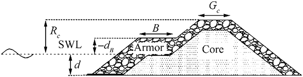Figure  1  Definition of cross-sectional parameters of a berm breakwater

Download: Full-Size Img

The wave overtopping distribution, the forces induced on infrastructures, and vehicles or people on the crown of the structure are also of great interest. Wave overtopping can bring troublesomeness or harm to people and property in various forms. EurOtop (2018) mentions four general categories under which the dangers of wave overtopping can be placed:

(1) The direct hazard of injury or death to people immediately behind the defending structure.

(2) Damage to property, operation, and/or infrastructure in the area defended, including loss of economic, environmental, or other resources or disruption to economic activity or process.

(3) Damage to defending structure(s), either short-term or longer-term, with the possibility of breaching and flooding.

(4) Low depth flooding (inconvenient but not dangerous).

In order to provide guidelines in the design of coastal structures, many empirical formulas based on the experiments have been developed in the past. Most of them are simple expressions describing overtopping discharges on rubble mound breakwaters, for example, TAW (2002), Owen (1980), Van der Meer and Janssen (1995), Besley (1999), Lykke Andersen (2006), and Moghim et al. (2015). The formulae for the spatial distribution of wave overtopping on rubble mound structures are also available in the literature, such as Jensen (1984), Lykke Andersen (2006), Van Kester (2009), Lioutas (2010), Krom (2012), and Sigurdarson and Van der Meer (2012). The aforementioned studies are based on experimental results. The most powerful empirical prediction method is the CLASH project that includes almost 10 000 experimental data collected all around the world (De Rouck 2005). Several formulae proposed for calculating the overtopping discharges on berm breakwaters are cited here.

Lykke Andersen (2006) carried out experimental model tests on berm breakwater cross sections, with the stability conditions varying from non-reshaping to fully reshaping. The overtopping volume was measured at the lee-side of the crest once the tested profiles were reshaped and stabilized for the applied wave conditions. The formula for q^· is given as

where

where q is the overtopping discharge per meter of structure width, g is the acceleration due to gravity, R_c is the crest freeboard which is the vertical distance from SWL to the point where the overtopping is measured, G, d_B, and B are the crest width, berm level, and berm width, respectively. f_Ho accounts for the influence of stability number, T_o is the dimensionless wave period, T_{0, 1} is the mean wave period based on frequency domain analysis, T_p is the period corresponding to the spectral peak frequency, T_o^· is the dimensionless wave period, s_om is the mean wave steepness, and H_oT_o is the stability number including mean wave period.

Van der Meer and Janssen's (1995) formula was developed using model test data, which represented dikes, revetments, and seawalls. It is expected to well predict the overtopping discharge on reshaped berm breakwater profiles by using their overtopping formula. This formula is later slightly modified and presented by TAW (2002). TAW formula is also reported in the EurOtop manual as the following for berm breakwaters (2018):

where ξ₀ is the breaker parameter $ \left({\xi}_{\mathrm{o}}=\tan\;\alpha /\sqrt{S_{\mathrm{o}\mathrm{m}}}\right),\kern0.5em {T}_{\mathrm{m}} $ is the mean wave period, α is the slope angle, γ_b is the reduction factor for a berm, γ_v is the reduction factor for a vertical or nearly vertical crown wall, γ_f is the reduction factor for roughness and permeability, and γ_β is the reduction factor for wave direction (EurOtop 2018).

Existing formulae for calculating the wave overtopping distribution on rubble mound breakwater are cited below.

Lykke Andersen (2006) carried out physical model tests to investigate the spatial distribution of wave overtopping discharge for multiple configurations of rubble mound breakwaters with a crest wall. Their study mainly focused on the distribution of overtopping traveling through the air and landing on the area behind the crest wall. The distribution depends on the level for the rear side of the crest wall and the distance from this rear wall. The coordinate system ($ \hat{x} $, $ \hat{y} $) starts at the rear side and the top of the crest, see Figure 2. The distribution of the wave overtopping discharge and the travel distance $ \hat{x} $ (at a certain level $ \hat{y} $) could be described by Eq. (13). The exceedance probability (F) of the travel distance is defined as the volume of overtopping water passing a given $ \hat{x} $- and $ \hat{y} $-coordinate, divided by the total overtopping volume. The probability, therefore, lies between 0 and 1, with F = 1 at the top of the crest wall.

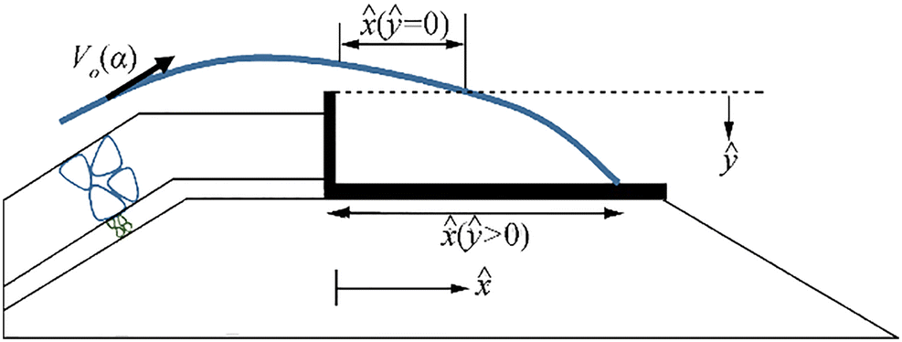Figure  2  Definition of $ \hat{x} $- and $ \hat{y} $-coordinate system (Lykke Andersen 2006)

Download: Full-Size Img

where β is the angles of wave attack.

Van Kester (2009) performed experimental research to investigate the spatial distribution of wave overtopping for both impermeable and permeable backfill without crest wall while using regular waves. The results are shown below:

Impermeable backfill

Permeable backfill

where $ {H}^{\cdotp }{T}^{\cdotp }=\left({H}_{\mathrm{m}\mathrm{o}}/{R}_{\mathrm{c}}\right){T}_{\mathrm{m}}\sqrt{g/{R}_{\mathrm{c}}},\kern0.5em q\cdotp \left(\hat{x}\right)=q\left(\hat{x}\right)/\sqrt{gH_{\mathrm{m}\mathrm{o}}^3}, $ is the dimensionless overtopping discharge at a certain distance $ \hat{x} $ behind the crest, $ {q}_{\mathrm{bc}}^{\cdotp }={q}_{\mathrm{bc}}/\sqrt{gH_{\mathrm{mo}}^3} $ is the dimensionless overtopping discharge directly behind the crest $ \left(\hat{x}=0\right),\kern0.5em q\left(\hat{x}\right) $ is the overtopping discharge at the location $ \hat{x} $ and q_bc is the overtopping discharge directly behind the crest.

Krom (2012) carried out experimental research to study the spatial distribution of overtopping volumes at hardly or non-reshaping berm breakwater while using irregular waves with a JONSWAP spectrum. Experiments were performed in the "Lange Speurwerk Goot" in the Fluid Mechanics Laboratory of the Delft University of Technology. The wave flume was 40 m long, 0.8 m wide, and nominally 0.9 m deep. A wavemaker existed at one side of the wave flume with three wave gauges, which were equipped with an active reflection compensator to measure reflected waves and also adjust the motion of the wave generator. The overtopped water was collected in eight bins, which are filled with core material (Figure 3). Table 1 shows the position of the collection bins. Eight pumps (one for each bin) transport the water-related to overtopping to floating collection tanks at the very end of the wave flume. Eventually, the overtopping discharge was given by measuring the weight of each collection tank for eight locations. An overview of dimensional parameters and also material properties involved in the experiments are given in Table 2 and Table 3 (Krom 2012).

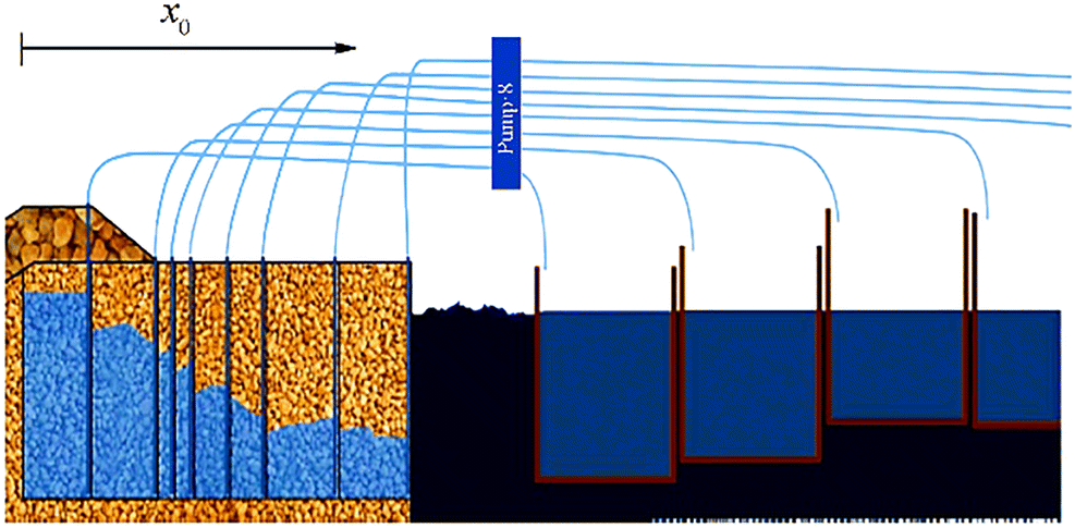Figure  3  The setup of measuring system (Krom 2012)

Download: Full-Size Img

The major part of Krom data represented submerged berms, while only one emerged berm level (d_b = − 0.1 m) was studied in his study. Nevertheless, the berm breakwaters are usually designed and constructed with emerged berms (d_b < 0). The developed formula is similar to that of the one reported in EurOtop, as shown below (Krom 2012):

The value of γ_f can be used from EurOtop (2018). In fact, the Krom formula is less popular because it was developed from tests with submerged berms (d_b > 0), and the only one emerged berm level configuration was tested.

These empirical formulations have been the main tools for coastal structural design. However, they are based on experimental works covering a limited number of typologies and setups. Their use out of the validity range, a problem often faced for design, may require extrapolations increasing uncertainties. To overcome these limitations, the numerical modeling of wave interaction with breakwaters has been used as a complementary approach during the last decade (Losada 2003).

Nowadays, researchers get interested in numerical simulation. Low-cost setups and limitless domain of computations encourage scientists to use numerical methods. The most popular models are based on different forms of the non-linear shallow water equations (NSWE), e.g., Kobayashi and Wurjanto (1989), Mingham and Causon (1998), Hu et al. (2000), Stansby and Feng (2004), Ingram et al. (2009), and Tuan and Oumeraci (2010), which provide efficient tools on evaluating the overtopping discharge. The NSWE is derived on the assumption of hydrostatic pressure and obtained by vertically integrating the Navier-Stokes equations. However, depth-integrated equations cannot be expected to accurately capture the wave breaking, turbulence transportation, and significant vertical component of velocity.

The second method is based on the smooth particle hydrodynamics (SPH) method (Gotoh et al. 2004; Shao et al. 2006), and the third method is based on RANS (Reynolds Average Navier-Stokes) model which includes VOF technique to compute large free surface deformations. The last method has made great improvement and becomes a dominant numerical approach that can provide a more comprehensive and detailed description of wave overtopping process, especially for violent breaking waves on the structure. Several researchers have been working on this type of model such as Troch and De Rouck (1998), Soliman (2003), Li et al. (2004), Lara et al. (2006), and Losada et al. (2008).

Liu et al. (1999) presented a RANS (Reynolds-Average Navier-Stokes) model, nicknamed COBRAS (Cornell Breaking Waves and Structures), to simulate breaking wave overtopping a porous media. The corresponding turbulence field being modeled by an improved k-ε model (Liu et al. 1999). The model was validated for a vertical caisson protected by an armored layer made of tetrapods in a very small computational domain (7.348 m × 0.43 m) and for a very short simulation time (18.2 s) under the influence of 13 regular waves.

Losada et al. (2008) improved the COBRAS model that nicknamed UC-COBRAS at the University of Cantabria by investigating the interaction of random waves with rubble mound breakwaters, especially wave overtopping rate. A total number of 45 tests with random and regular waves were generated in their experiments to simulate sea states, which produced large overtopping events. They solved porous media flow in VARANS (Volume-Averaged Reynolds-averaged Navier-Stokes) equations by including the extended Forchheimer relationship in the momentum equations. Extended Forchheimer's relationship includes linear and non-linear drag forces using two empirical coefficients α and β. Losada et al. (2008) analyzed wave overtopping discharge using this model, and a good agreement in their simulation was concluded.

Although various numerical models have been studied for overtopping problems, details of the wave overtopping distribution studies are still under development, especially for berm breakwaters. It should be noted that the average overtopping rate alone is not enough to analyze the functionality of the structure. Rather more information about wave overtopping distribution, which is a crucial factor in evaluating the stability of the crest and rear side of the breakwater, is needed. Also, the previous empirical overtopping formulae calculated only the mean overtopping at the top of the breakwater crest, while the tolerable overtopping discharges are defined at a certain point behind the crest where the total overtopping is reduced.

3   Numerical Model

3.1   Governing Equations

The present numerical simulation is based on RANS equations, the governing equations can be written as

where $ {\overline{u}}_{\mathrm{i}} $ and $ {\overline{u}}_{\mathrm{j}} $ are the time average velocity components, i, j = 1, 2, 3, representing the horizontal directions x and y, and the vertical direction z, respectively; p is the pressure intensity, μ is the dynamic viscosity of fluid, ρ is the fluid density, and f is the unit body force.

According to the Boussinesq hypothesis, the Reynolds stress term $ \left(\overline{u_{\mathrm{i}}^{\prime }{u}_{\mathrm{j}}^{\prime }}\right) $ in Eq. (20) can be written as

where k is the turbulent kinetic energy, δ_ij is the Kronecker delta function such that δ_ij = 1 when i = j; δ_ij = 0, when i ≠ j and $ {\upsilon}_{\mathrm{t}}={}^{{{\mu }_{\text{t}}}}\!\!\diagup\!\!{}_{\rho }\; $.

The renormalization group (RNG) k-ε turbulence model was used to close the governing equation (Yakhot and Orszag 1986). This turbulence model consists of two equations.

The turbulent kinetic energy k equation:

The turbulent dissipation rate ε equation:

in which $ {\mu}_{\mathrm{t}}={C}_{{\rm{ \mathsf{ μ} }}}\rho \frac{k^2}{\varepsilon } $ is the turbulence viscosity. $ {p}_{\mathrm{k}}={\mu}_{\mathrm{t}}{S}^2,\kern0.5em S=\sqrt{2{S}_{\mathrm{i}\mathrm{j}}{S}_{\mathrm{i}\mathrm{j}}},\kern0.5em {S}_{\mathrm{i}\mathrm{j}}=\frac{1}{2}\left(\frac{\partial {\overline{u}}_{\mathrm{i}}}{\partial {x}_{\mathrm{j}}}+\frac{\partial {\overline{u}}_{\mathrm{j}}}{\partial {x}_{\mathrm{i}}}\right),\kern0.5em {R}_{{\rm{ \mathsf{ ε} }}}=\frac{C_{{\rm{ \mathsf{ μ} }}}{\rho \eta}^3 \left( 1-{}^{\eta }\!\!\diagup\!\!{}_{{{\eta }_{\text{o}}}}\; \right)}{1+{\beta \eta}^3}\frac{\varepsilon^2}{k}, $ and $ \eta =\frac{Sk}{\varepsilon }. $ The constant values were used as follows: σ_k = 0.7194, σ_ε = 0.7194, C_ε1 = 1.42, C_ε2 = 1.68, C_μ = 0.085, η_o = 4.38, and β = 0.012 (Orszag et al. 1996). One of the major advantages of the RNG theory is that the important turbulent coefficients are theoretically determined rather than being adjusted empirically.

The VOF method is used to capture free surface, and the VOF transport equation is expressed as (Hirt and Nichols 1981)

where α is the volume of fraction indicating the relative proportion of fluid in each cell, and it always ranges between 0 and 1.

In this paper, the governing equations with the above-described computational domain and simulation setup are discretized by the finite-volume method on staggered grids. In particular, the implicit, GMRES pressure solver and explicit viscous stress solver is used. First-order momentum advection is selected, and the split Lagrangian method is employed to resolve the volume of fluid advection.

3.2   Wave Flume

As the free surface time series were not available in the Krom (2012) experiments, the theoretical results have been used to validate the numerical wave flume with the free surface time series ensuring the numerical model performance in the wave generation. To achieve these goals, at first, the targeted regular waves from theory with a vertical wall at the end of the flume were simulated. Afterward, the simulation of the targeted irregular wave with the JONSWAP spectrum in the flume with a wave absorber at the end of the flume was carried out.

Simulations are performed in 2D (1 cell in the transverse direction). A numerical wave flume was set up in order to carry out the numerical simulation based on typical experimental arrangements. To identify boundary conditions in a computational domain, the user-defined wave energy spectrum was prescribed for the wave boundary condition of the numerical simulation with the aim of generating the irregular waves. The energy spectrum is defined with a series of angular frequencies of waves (in rad/time), and the corresponding energy values. An active absorption is employed to avoid re-reflective at the wave generation boundary. The solid obstacles within the numerical domain (i.e., the bed flume) are modeled as 'no-slip', and for the rest, boundary conditions are declared symmetrically. At the end of the longitudinal direction of the numerical irregular wave flume, the boundary condition was declared an outflow boundary, which is useful when modeling in the presence of linear surface waves at this boundary.

Regular Wave with a Vertical Wall at the End of the Flume If a progressive regular wave was a normal incident wave on a vertical wall, it would be reflected backward without any changes in its height. This can be explained by a standing wave with the reflection coefficient (k_r = H_r/H_i, H_r, and H_i are the reflected and incident wave heights) of 1 in front of the wall. The piston-type numerical wavemaker using FLOW-3D is utilized to generate the incident wave as a wave boundary condition, and the wavemaker is forced to create the sinusoidal motions to simulate the regular harmonic waves. At the outlet and also at the bottom of the flume, the no-slip wall boundary condition is imposed. The numerical wavemaker generates a regular wave in which the wavelength is 3.781 m, the wave height is 0.175 m, and the wave period is 1.67 s. The validation is conducted by comparing the simulated wave and the Stokes (5th-order theory) wave elevation based on LeMehaute (1969).

The length, width, and height of the simulated flume are 15 m, 0.4 m, and 1.2 m, respectively, and the initial fluid elevation was 0.8 m. The length of the flume is proportional to wavelength, which provides sufficient time for the simulator to generate the required number of wave encounters before the first wave reaches the outflow boundary (Thanyamanta et al. 2011).

A structured mesh is used to discretize the computational domain. To determine an appropriate mesh size in the flume, the incident wave interaction with the vertical wall at the end of the flume is chosen to carry out the mesh independence check. The grid is evenly distributed in the whole computational domain. Three meshes were used: finest mesh size 0.015 m, fine mesh size 0.022 m, and coarse mesh size 0.03 m. Figure 4 shows instantaneous water surface displacements and envelope in a standing wave for mesh size 0.015 m. From the recorded wave envelope and by using the following relationships, the reflection coefficient is determined:

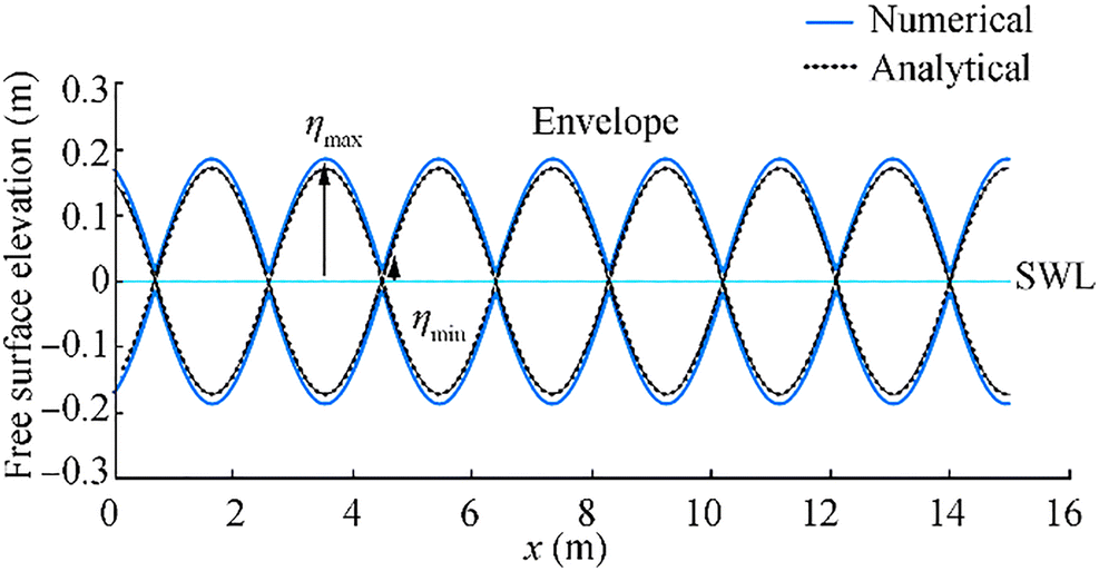Figure  4  Instantaneous water surface displacements and envelope in a standing wave for mesh size 0.015 m (H_i = 0.175 m, T = 1.67 s, and d = 0.8 m)

Download: Full-Size Img

where H_i is the incident wave height, H_r is the reflected wave height, η_min is the wave height at the node of the wave envelope, and η_max is the wave height at the antinode of the wave envelope.

Table 4 lists the grid sensitivity analysis for generating a wave in the numerical wave flume with a vertical wall at the end. It is observed that the obtained results for k_r have a good convergence with the decrease of the mesh size for which a reflection coefficient close to 1 denotes the best result. To improve the calculation efficiency while the accuracy is guaranteed, the square mesh size of 0.015 m is selected.

Irregular Wave with a Wave Absorber at the End of the Flume The numerical wavemaker generates an irregular wave with a JONSWAP spectrum with a significant wave height of 0.1218 m and a peak wave period of 3.56 s at the water depth of 0.5 m. The length, width, and height of the simulated flume are 13.2 m, 0.4 m, and 1.4 m, respectively. The boundary conditions are the same as the aforementioned section, except for the outlet of the domain that is a wave damping region (i.e., the sponge layer) which is capable of absorbing waves, reduce reflections at the outflow boundary, and also, maintain the fluid volume in the domain. The wave boundary condition that comes up to standard with FLOW-3D generating an irregular wave is a user-defined wave energy spectrum. The energy spectrum file has two columns, where the left one is a series of angular frequencies of waves (in rad/time), and the right column is the corresponding energy values. Based on the numerical simulations performed for regular waves, a uniform grid size of 0.015 m is hired in the domain. The validation is carried out by comparing the simulated wave and the JONSWAP wave spectrum with the peak enhancement factor of γ = 3.3. With the aim of generating the JONSWAP wave spectrum, the wind speed needs to be as the input parameter. Experimental data presented by Krom (2012) only have the significant wave height and the peak wave period available. Goda (1988) presented the following equation to generate the JONSWAP wave spectrum by using wave height and period:

in which S(f) is the wave spectral density function, f is the frequency, H_1/3 is the significant wave height, γ is called the peak enhancement factor being given the value of 3.3, σ is the constant having the value of 0.07 for f ≤ f_p and 0.09 for f > f_p and β_j is (Goda 1988)

Forty-five linear wave components are considered to generate the irregular target wave. The numerical simulations were run for 200 s, and the results were compared with the wave spectrum of the corresponding data by Goda (1988) theory. Figure 5 indicates the corresponding wave spectrum of H_s = 0.1218 m and T_p = 3.56 s for numerical simulation and Goda theory. The agreement between numerical results and experimental data is reasonable.

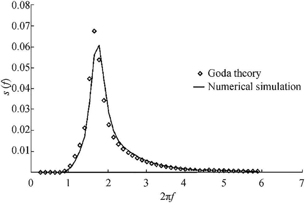Figure  5  Comparison of wave spectrum corresponding H_s = 0.1218 m and T_p = 3.56 s between Goda theory and numerical simulation

Download: Full-Size Img

3.3   Breakwater Model Setup

Following the experimental setup presented in Krom (2012), the computational domain of the numerical wave flume and berm breakwater is shown in Figure 6. The geometry of the berm breakwater includes a seaward slope of 1:2, a berm width of 0.3 m, a berm height (d_B) of − 0.08 m, a crest width of 0.18 m, and a height of 0.52 m. Other parameters, such as material properties and sea state parameters, are listed in Tables 2 and 3. Figure 6 depicts the breakwater model with an unusual core configuration based upon Krom's experimental model to measure the spatial distribution of wave overtopping. As Krom (2012) stated in his report, the filtration can probably influence the spatial distribution of overtopped water over the breakwater crest. The same configuration has been reproduced here to compare the numerical results to the observed data. The numerical wavemaker generates an irregular wave with the JONSWAP spectrum in which the significant wave height is 0.1218 m, and then the mean wave period is 2.96 s at a water depth of 0.5 m. A uniform grid size of 0.015 m is used in the domain. In FLOW-3D codes, the baffle acts as the flux surface diagnostic tool in computing flow rate quantities for a simulation. To measure wave overtopping, horizontal flux surfaces (baffles) are installed at certain positions of the breakwater crest lee-side. The baffle positions in Figure 6 are based on the position of the collection bins from Table 1. The baffle can derive the flux (m³/(s•m^-1)) through its surface in time.

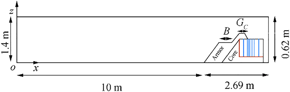Figure  6  The computational domain of the numerical wave flume and berm breakwater

Download: Full-Size Img

The porous media flow in the RANS equations is modeled by including the extended Forchheimer relationship in the momentum equations, in which both linear and non-linear drag forces are considered. The expression used in the model for the linear and non-linear drag forces is given by:

where I is the hydraulic gradient, and α and β are the only two empirical parameters used in the numerical model calibration, n is the porosity, ν the kinematic viscosity, and u stands for the velocity. The precise descriptions of α and β coefficients are still not fully understood for oscillatory flows. They depend on several parameters such as the Reynolds number, the shape of the rocks, the grade of the porous material, the permeability, and of course, the flow characteristics. Several researchers have suggested different values (e.g., Shih 1990; Van Gent 1995; Burcharth and Andersen 1995). However, when comparing different formulations, attention must be drawn to the facts that discrepancies may exist in the expressions of the terms, and the value of parameters depends on the flow conditions. In this work, the formula which was proposed (derived) by Shih has been used as following (Shih 1990):

Losada et al. (2008) found that the numerical results appeared to be more sensitive to the non-linear drag coefficient (β) than the linear drag parameter (α), because the flow is mainly turbulent. By using the rock diameter for armor (D_n50 = 0.062 m), β and α are 1.72 and 7180, respectively. For the core layer (D_n50 = 0.021 m), β and α are 1.88 and 2314, correspondingly. In this study, the best-fit values for the porosity (n) are evaluated by comparing experimental data and numerical results of wave overtopping distribution for irregular wave case. As the first attempt, the porosity value is considered 0.40 for the armor layer and 0.30 for the core layer.

Aiming at finding the proper time to simulate the numerical model, the model is run for 50 s, 100 s, 150 s, 200 s, 400 s, and 1140 s by performing different simulations. It should be noted that the test duration for the mentioned wave condition was considered to be 1140 s. The volume of overtopped water is calculated for unit-width of each bin during the run time, and the averaged overtopping discharge for the unit-width is calculated. The results are tabulated in Table 5. It can be seen that for the aforementioned irregular wave condition, the averaged overtopping discharge becomes unchanged after 200 s. Therefore, simulations limited to 200 s will be used to represent wave overtopping processes to save computational time.

To evaluate the appropriate mesh size, validation indices are used. These validation indices are based on normalized root mean square error (NRMSE), percentage of relative error (E), and the square of the correlation factor (R²). These are computed according to

where O is the numerical result, P is the experimental data, $ \overline{O} $ is the average value for the numerical result, $ \overline{P} $ is the average value for the experimental data, and N is the total number of bins. Appropriate mesh size is determined by performing mesh independence check on the irregular wave interactions with the berm breakwater. The selected significant wave height is 0.1218 m, and the mean wave period is 2.96 s. The volume of wave overtopping distribution at different bin numbers is simulated. Table 6 shows the validation indices for the volume of wave overtopping distribution in each bin with different mesh sizes against Krom (2012) experimental data. It is observed that the decline of mesh size results in better convergence in the outcomes. In the current study, the mesh size of 0.013 m is adopted to improve the calculation efficiency while the accuracy is guaranteed. The total number of cells is 3.3 million. The numerical simulations were run for 200 s corresponding to the experimental data.

3.4   Model Calibration

To determine the proper porosity and to calibrate the numerical model, the volume of overtopped water in a run time of 200 s was calculated for each bin. The model calibration was performed using irregular waves with the JONSWAP spectrum. The significant wave height is 0.1218 m, and the mean wave period would be 2.96 s at a water depth of 0.5 m. A uniform grid size of 0.013 m is used in the domain. Different combinations of porosity for armor and core layer were selected, as listed in Table 7. The volume of wave overtopping distribution in unit width (1 m) is presented in each bin for different combinations of armor and core porosity. At the right side of the table, the equivalent volume of wave overtopping distribution in each bin is presented for 200 s test run from Krom (2012) experimental results in unit width.

Table 8 shows the values of the validation indices with different layers (either armor or core) porosity. It is evident that run No. 5 suggests that the best validation indices with the square of the correlation factor are about 99.9%, the NRMSE error and E error are about 0.056 and 0.068, respectively. Therefore, the best-fit values of volume of wave overtopping distribution calculated by numerical method achieve when the armor porosity is 0.45, and the core porosity is 0.31. It is noteworthy to mention that porosities can be used as tuning parameters to obtain better adjustment between numerical calculations and experimental data. However, the layer porosities remain constant for all the other numerical calculations to show the ability of the model in simulating the experiments with the lowest possible number of calibration coefficients.

3.5   Model Validation

The calibrated empirical parameters were used as tuning parameters to obtain better adjustment between numerical calculations and experimental data for a non-reshaping berm breakwater. The calibration parameters should remain constant for all the other numerical models indicating the ability of the numerical model to simulate the experiments. The numerical model has been evaluated for two irregular wave combinations which were not used before. For the first combination, significant wave height and mean wave period are 0.106 m and 2.75 s at a water depth of 0.5 m and for the second one significant wave height and mean wave period of 0.155 m and 1.47 s at a water depth of 0.5 m are used. Table 9 illustrates the validation indices for the volume of wave overtopping distribution in each bin for the two wave combinations against Krom (2012) experimental data. The comparison with the computational and experimental results highlights a very good agreement.

Throughout this section, the computational setup is presented. The model was calibrated based on comparisons with Krom (2012) experimental data, including wave overtopping distribution. Then, computations were validated against the experimental data by two other wave combinations. After model calibration and validation, in the following section, the model is used to predict wave overtopping distribution.

4   Wave Overtopping Distribution Analysis

In this section, the validated numerical model is used to model the wave overtopping distribution on a non-reshaping berm breakwater. In the first place, the effect of sea state and structural parameters on wave overtopping discharge is considered with numerical data for 200 s simulation time. Then a new empirical formula to estimate wave overtopping is derived by using non-dimensional parameters. The range of the dimensional parameters covered in the present research is listed in Table 10.

The berm breakwaters are typically designed and constructed with a berm above the SWL. As explained earlier in section 1, Krom's (2012) formula is not at the center of attention due to that the major part of Krom data represented for submerged berms. The present numerical results are comprised of cross-sections with the berm above SWL. The effect of berm height on wave overtopping discharge for different wave heights is shown in Figure 7. In the case of an increase in the berm height above still water level with the same wave height, the wave overtopping discharge will decrease.

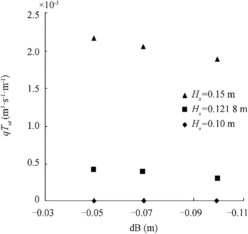Figure  7  Effect of berm height on wave overtopping discharge (B = 0.3 m, T_m = 2.96 s, R_c = 0.18 m, d = 0.5 m)

Download: Full-Size Img

The major part of Krom data represented submerged berms, while only one emerged berm level (d_b = − 0.1 m) was studied in his study. Nevertheless, the berm breakwaters are usually designed and constructed with emerged berms (d_b < 0).

4.1   Dimensionless Analysis

The main purpose of this section is to identify the proper dimensionless parameters and their influence upon the overtopping discharge. The same method used by Van der Meer (1988) and Moghim et al. (2015) is used herein. Similar results have been achieved by using non-linear fitting algorithms. It has to be stressed that the main purpose of the analysis is not merely to propose an empirical formulation to estimate the overtopping discharge. Rather, it aims to investigate the effect of each dimensionless parameters on the wave overtopping.

Employing Buckingham π-theorem, which is a key theorem in dimensional analysis for the spatial distribution of wave overtopping discharge for non-reshaping berm breakwater, will yield the following equation:

Since it has three fundamental physical dimensions in equation, it needs 11–3 = 8 dimensionless independent group. So, the equation can be re-stated as the following equation:

where $ {q}^{\cdotp}\left({x}_{\mathrm{o}}\right)=\frac{q\left({x}_{\mathrm{o}}\right)}{\sqrt{gH_{\mathrm{mo}}^3}},{T}^{\cdotp }={T}_{\mathrm{P}}\sqrt{\frac{g}{R_{\mathrm{c}}}},{d}_{\mathrm{B}}^{\cdotp }=\frac{d_{\mathrm{B}}}{H_{\mathrm{mo}}},{R}_{\mathrm{c}}^{\cdotp }=\frac{R_{\mathrm{c}}}{H_{\mathrm{mo}}},{B}^{\cdotp }=\frac{B}{H_{\mathrm{mo}}},{x}_{\mathrm{o}}^{\cdotp }=\frac{x_{\mathrm{o}}}{H_{\mathrm{mo}}},\operatorname{Re}=\frac{\rho \sqrt{gH_{\mathrm{mo}}}{D}_{50}}{\mu }, $ and $ {D}^{\cdotp }=\frac{D_{\mathrm{n}50}}{H_{\mathrm{mo}}}. $

The minimum Reynolds number value for these numerical results with the lowest wave height is Re = 4 × 10⁴. This value is greater than the critical value presented by Van der Meer (1988) and then it is feasible to omit the Reynolds number.

Figure 8 shows the variation of q^*(x_o) versus T^· for different non-dimensional locations $ \left({x}_o^{\ast}\right) $. Different functions have been fitted to each data set. Among different functions fitted to each set of data, exponential functions are the most accurate. Since other researchers have used the exponential function to estimate wave overtopping over the rubble mound breakwater, the same function has been considered in the present study to provide the estimation of each effective parameter. The function with the following form is fitted to each set of data.

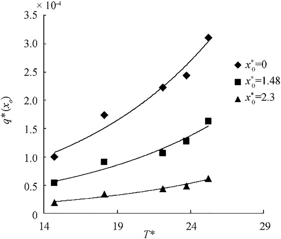Figure  8  Variation of q^*(x_o)versus T^* ($ {d}_B^{\ast }=0.821 $, B^* = 2.46, $ {R}_c^{\ast }=1.48 $)

Download: Full-Size Img

Values of coefficients in Eq. (35) for different values of $ {x}_o^{\ast } $ are presented in Table 11. It can be observed that for different values of $ {x}_o^{\ast } $, the value of c₁ is almost constant, and in order to accommodate the values for this coefficient, the average values are used, i.e., c₁ = 0.095. The value of α₁ is a function of $ {x}_o^{\ast } $. The following equation will be used as a proper pattern to consider the effect of T^· on q^· (x_o):

In order to achieve α₁, Eq. (36) can be rewritten as below:

Figure 9 shows the variation of α₁ against $ {d}_B^{\ast } $ for different non-dimensional locations $ \left({x}_o^{\ast}\right). $ Among different functions fitted to each data set, exponential functions behave in a most accurate way. The function with the following form is fitted to each set of data.

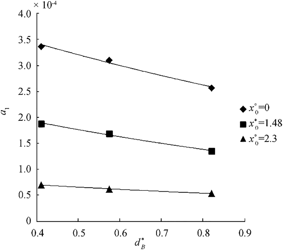Figure  9  Variation of α₁ versus $ \left(-{d}_B^{\ast}\right)\left({B}^{\ast }=2.46,{R}_c^{\ast }=1.48\right) $

Download: Full-Size Img

Values of coefficients of Eq. (38) for different values of $ {x}_o^{\ast } $ are presented in Table 12. It can be observed that for different values of $ {x}_o^{\ast } $, the value of c₂ is almost constant, i.e., c₂ = − 0.7. The value of α₂ is a function of $ {x}_o^{\ast }. $ The following equation will be used as a proper pattern to consider the effect of $ {d}_B^{\ast } $ on α₁:

In order to designate α₂, the Eq. (39) can be rewritten as the following:

Figure 10 shows the variation of α₂ versus B^* for different non-dimensional locations $ \left({x}_o^{\ast}\right). $ Among different functions fitted to each set of data, exponential functions give the most precise behavior. The former method is used to achieve the following equation as a proper pattern to consider the effect of B^* on α₂:

Figure  10  Variation of α₂ versus $ {B}^{\ast}\left({R}_c^{\ast }=1.48\right) $

Download: Full-Size Img

In order to designate α₃, the Eq. (41) can be rewritten as the following:

Figure 11 shows the variation of α₃ versus $ {R}_c^{\ast } $ for different non-dimensional locations $ \left({x}_o^{\ast}\right). $ Among different functions fitted to each set of data, exponential functions were the most accurate. The previous method is used to obtain the following equation as a proper pattern to consider the effect of $ {R}_c^{\ast } $ on α₃:

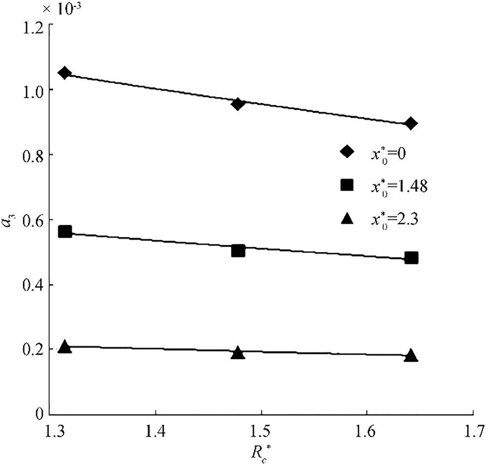Figure  11  Variation of α₃ versus $ {R}_c^{\ast } $

Download: Full-Size Img

In order to designate α₃, the Eq. (43) can be rewritten as the following:

Figure 12 shows the variation of α₄ versus $ {x}_o^{\ast } $ for all numerical results. Among different functions fitted to each set of data, exponential functions are the most accurate as follows:

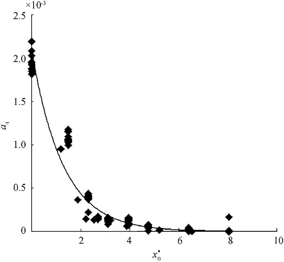Figure  12  Variation of α₄ versus $ {x}_o^{\ast } $

Download: Full-Size Img

Using non-linear regression leads us the following equation:

By substituting Eqs. (37), (40), (42), and (44) in Eq. (46), the following formula is obtained to calculate the wave overtopping distribution for a non-reshaping berm breakwater.

Based on experimental work limitations, Eq. (47) is valid for:

It should be noted that the total overtopping discharge per meter of structure width (q) can be evaluated as the integral of the proposed equation for q(x_o) over x_o.

Figure 13 shows the dimensionless value of total overtopping discharge per meter of structure width (q^·) from numerical results against the calculated dimensionless value of overtopping discharge (q^·) with the new formula (Eq. 47). To draw a fair comparison in Figure 13, the current experimental data which were not employed in the derivation of Eq. (47) is used. The square of the correlation factor between numerical results and calculated dimensionless wave overtopping discharge is about 99.3%, while the NRMSE error and E error are about 0.121 and 0.07, respectively. This quantification may well be interpreted as a "very good" agreement.

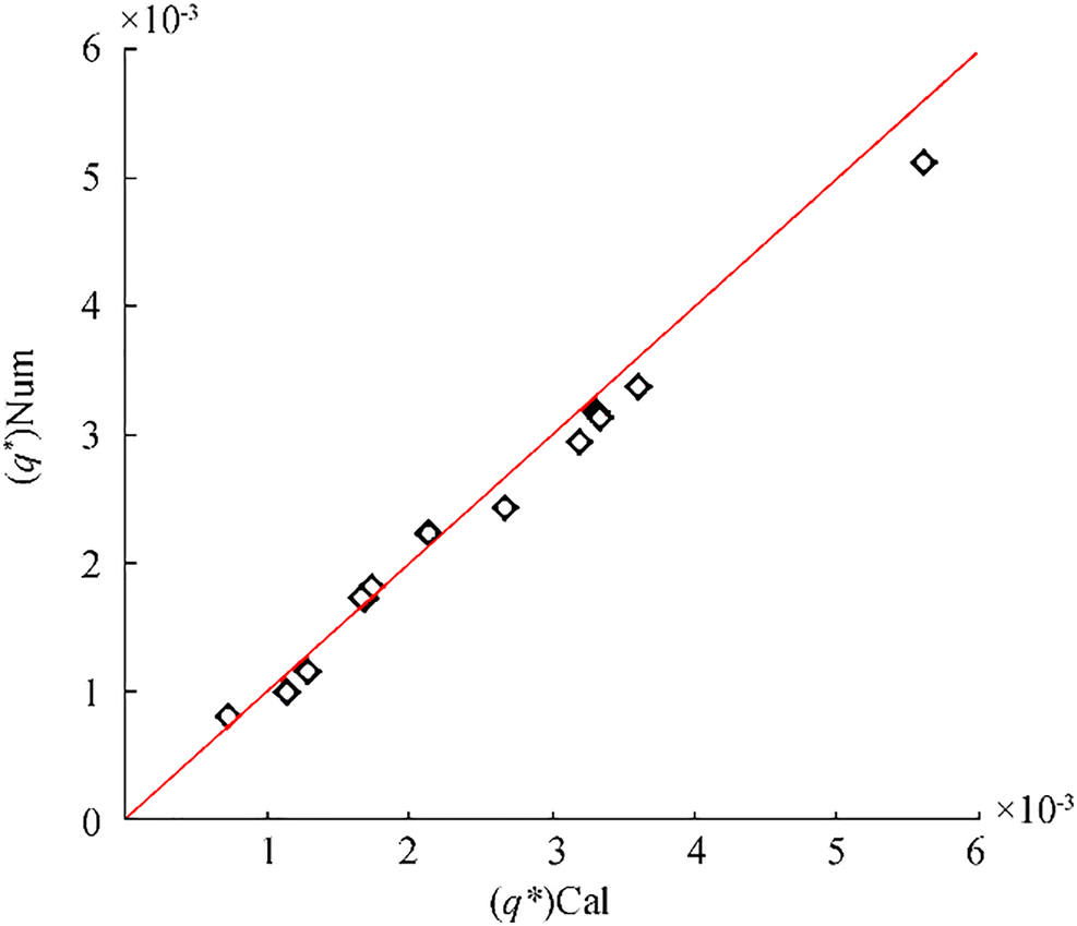Figure  13  Comparison of numerical results and calculated value of dimensionless total overtopping discharge with new formula

Download: Full-Size Img

4.2   Validity Investigation of the New Formula with Other Researchers' Formulae

In this section, the validity of the new empirical formula to predict the total wave overtopping discharge per meter of structure width for non-reshaping berm breakwaters is evaluated. To show the prediction capability of the new formula in comparison with the earlier formulae, the validation indices for three available formulae are investigated against all numerical data.

Table 13 shows the values of the validation indices for available formulae against numerical data of wave overtopping discharge (q^·). The square of the correlation factor between numerical and calculated results with the new formula is more, and the NRMSE error and E error are less than other formulae. Figure 14 shows the dimensionless value of total overtopping discharge from numerical results against the calculated dimensionless value of total overtopping discharge with all formulae.

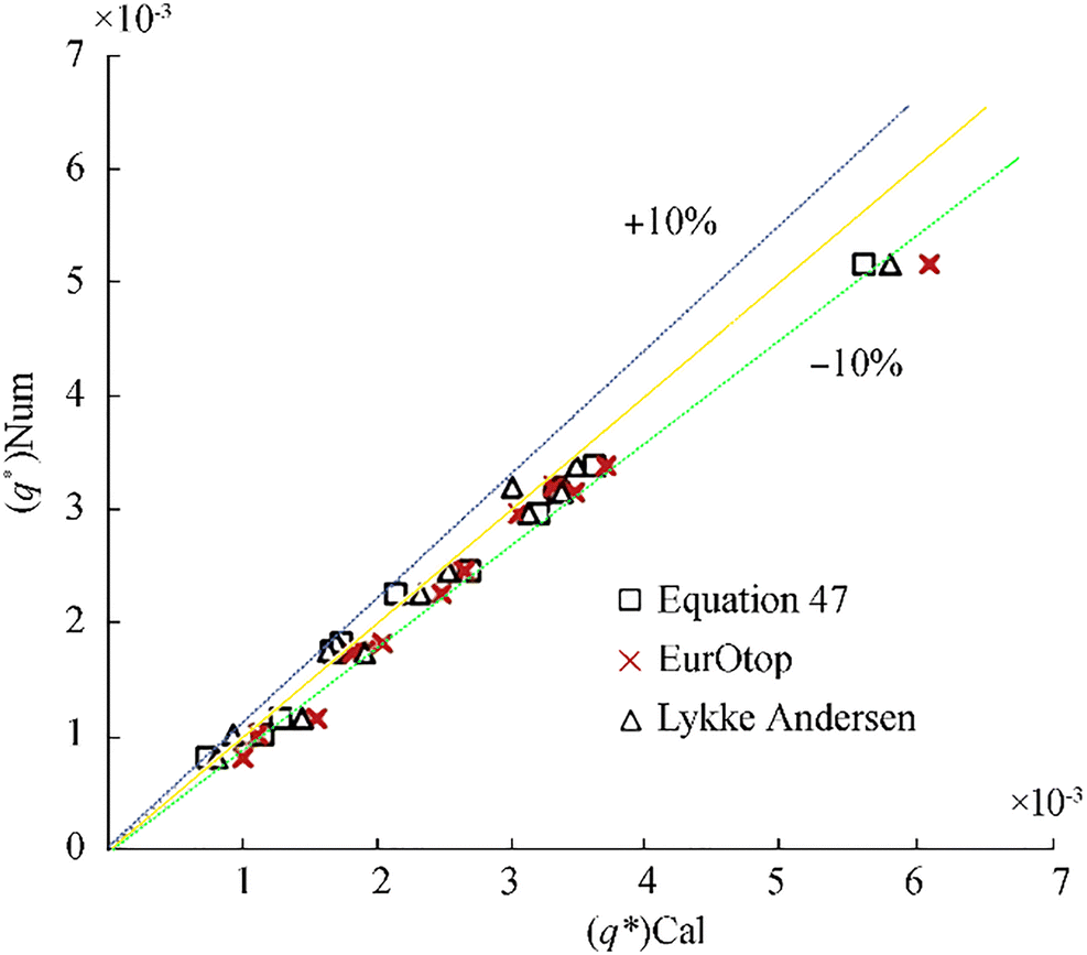Figure  14  Comparison of numerical results and calculated value of dimensionless total overtopping discharge with other formulae

Download: Full-Size Img

Also, the validity of the empirical new formula to predict the wave overtopping distribution in different locations of non-reshaping berm breakwaters is investigated. In order to show the prediction capability of the new formula in comparison with earlier formulae, the validation indices for four available formulae are investigated against all numerical data. All of the formulae were derived from calculating wave overtopping distribution of conventional breakwaters except the Krom (2012) and present formula (Eq. 47) that were derived for non-reshaping berm breakwaters. Figure 15 shows the dimensionless value of overtopping distribution from numerical results and calculated dimensionless value of overtopping distribution with all formulae versus a dimensionless parameter$ {x}_o^{\ast } $.

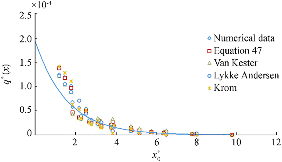Figure  15  Comparison of numerical results and calculated value of dimensionless wave overtopping distribution with other formulae

Download: Full-Size Img

Table 14 shows the values of the validation indices for available formulas against numerical data of wave overtopping distribution. The square of the correlation factor between numerical and calculated results with the new formula is higher (= 0.964), and the NRMSE error (= 0.161) and E error (= 0.09) are lower than other formulae.

4.3   Validity Investigation of the New Formula with Krom Data

The validity of the empirical new formula to predict the wave overtopping distribution in different locations of hardly or non-reshaping berm breakwater berm breakwaters is investigated with Krom experimental data. As the major part of Krom data represented submerged berms, the only one emerged berm level was studied in his study which is used in this section to investigate the validity of the new formula (Eq. 47). Figure 16 shows the dimensionless value of overtopping distribution from Krom data and calculated dimensionless value of overtopping distribution with Eq. (47) and Krom formula versus a dimensionless parameter$ {x}_o^{\ast } $. Table 15 shows the values of the validation indices. The square of the correlation factor between observed and estimated overtopping distribution is about 95.0%, while the NRMSE error and E error are about 0.18 and 0.10, respectively. This quantification may well be interpreted as "very good" agreement.

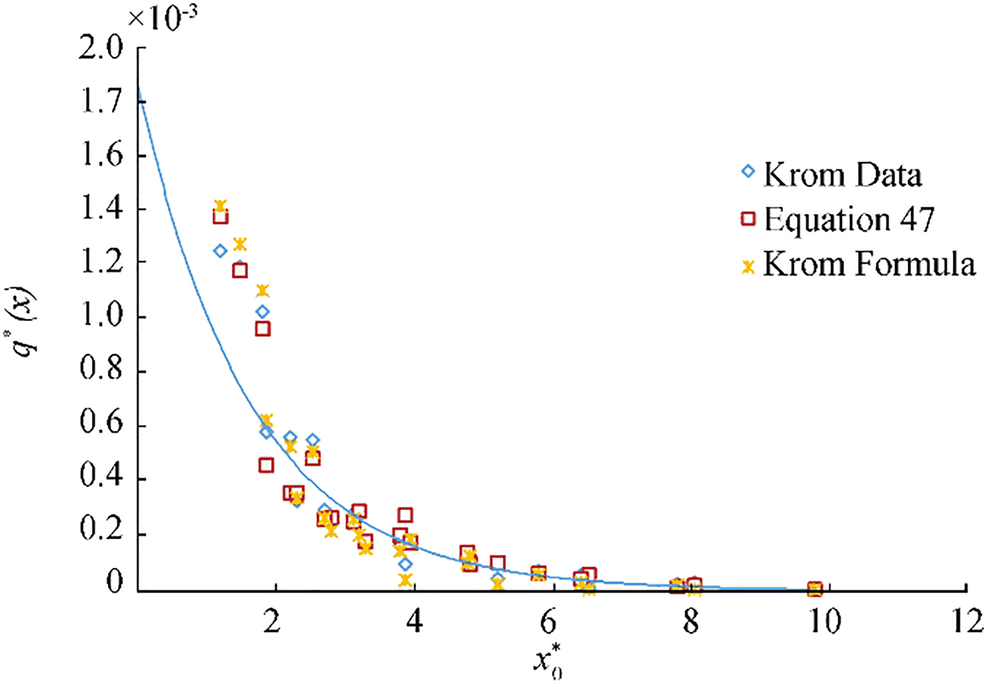Figure  16  Comparison of Krom experimental results and calculated value of dimensionless wave overtopping distribution

Download: Full-Size Img

4.4   Validity Investigation of the New Formula with Lykke Andersen Data

In this section, the validity of the new formula to predict the total wave overtopping discharge of non-reshaping berm breakwaters is evaluated versus Lykke Andersen (2006) formula. The validation indices are computed by using Lykke Andersen (2006) data. The data extracted from the Lykke Andersen data set are only those in the range of the present studies (structural geometry and sea state as given by Eq. 48). Table 16 shows the values of the validation indices. The results from Eq. (47) give more error than the Lykke Andersen's formula; however, the validation indices are within an acceptable range.

It is worth noting that Lykke Andersen's formula has been derived from his own experimental data, and his formula is expected to perform better than the existing formula for his data. Furthermore, Lykke Andersen's formula is only applied to calculate the overtopping discharge of berm breakwater, but the present formula is also capable of calculating the wave overtopping distribution of non-reshaping berm breakwaters. Figure 17 draws a comparison between the experimental and calculated value of overtopping discharge for the partial Lykke Andersen data satisfying Eq. (47).

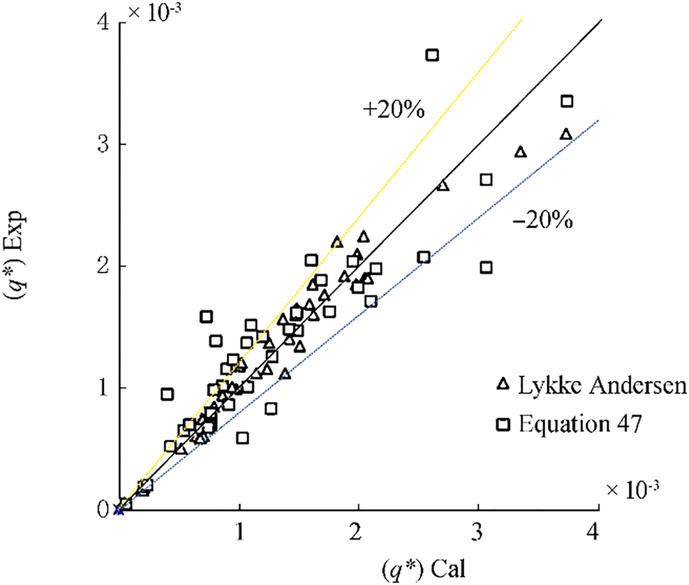Figure  17  Comparison of experimental results and calculated value of overtopping discharge for the partial Lykke Andersen data

Download: Full-Size Img

5   Conclusions

In this study, the distribution of irregular wave overtopping behind non-reshaping berm breakwaters was investigated by means of a RANS-VOF model. Numerical results were validated by Krom (2012) experimental data. Based on the numerical simulation of an experimental model under an irregular wave attack, it can be concluded that the model is capable of predicting the wave overtopping distribution of non-reshaping berm breakwaters. The validated numerical model was applied to investigate the effect of sea state and structural parameters on wave overtopping distribution of non-reshaping berm breakwaters. The following conclusions can be drawn from the present study:

(1) A new formula was derived to relate the spatial distribution of wave overtopping behind non-reshaping berm breakwaters to non-dimensional forms of wave height, wave period, berm width, berm height, and armor freeboard as an exponential function. This formula model agreed reasonably well with numerical model results.

(2) The prediction capability of the new formula is investigated by comparing with Lykke Andersen's formula using his experimental data in the range of the effective parameter in the present study. The error of the proposed formula is high if compared to the error of the Lykke Andersen's formula, but the validation indices were within an acceptable range. However, it is interesting to note that Lykke Andersen's formula has been derived for his data, and it is self-evident that his formula performs better than our formula for his own data set. Furthermore, Lykke Andersen's formula was only applied to calculate the overtopping discharge of berm breakwater, but the new formula presented in this study also has the ability to be used for calculating the wave overtopping distribution of non-reshaping berm breakwaters.