1   Introduction

In wireless communication systems, unknown channels will introduce an intersymbol interference (ISI) to reduce communication quality. A common method for eliminating ISI is to add a known sequence as a training sequence in the transmitted signal. Then, the training sequence is used to equalize the ISI (Ghofrani et al. 2018; Qiao et al. 2017). In the field of system identification, such as seismic inversion, no training sequence exists in the measured signal. Also, a direct measurement of a transmission channel is infeasible. In these scenarios, techniques for directly identifying a channel or system from observations need to be developed. Blind channel identification identifies channels that rely solely on a received channel output signal and certain a priori statistical knowledge (e.g., whiteness) of the source. Thus, blind channel identification can be used in scenarios where the source signal or system impulse response function cannot be directly obtained. In a radar communication system, a blind identification method can estimate a channel in real time without a training sequence, thereby saving channel resources and improving communication efficiency.

Sato presented a blind identification algorithm (Sato 1975) in 1975, thereby giving rise to the emergence of numerous blind identification algorithms. Classical blind identification techniques are mainly divided into three categories: methods based on higher-order statistics (HOS) (Friedlander and Porat 1990), subspace decomposition (Abed-Meraim et al. 2002), and second-order statistics (SOS) (Kailath et al. 1994). HOS-based methods can suppress Gaussian noise effectively, but most of these methods can be used in single-input single-output (SISO) systems only. HOS-based methods are sensitive to parameter settings, slow to converge, and require extensive observation times. Subspace-based methods can almost fully identify a channel when the signal-to-noise ratio (SNR) is high, but the estimation error increases rapidly when the SNR is reduced. Furthermore, subspace-based methods require accurate channel order estimation, which is difficult. SOS-based methods, such as constant modulus algorithm (A.-J V et al. 1996), least squares smoothing (Tong and Zhao 1999), linear prediction algorithm (LPA) (Zhang 2011), multi-step prediction (Duhamel and Gesbert 1997), and OPDA (Ding 1996; Ding 1997), have a higher estimation error level than subspace-based methods at high SNRs; however, these methods still perform effectively at low SNRs and are insensitive to channel order estimation errors. Therefore, SOS-based methods have high practical value.

Many new methods and applications have emerged in the field of blind identification in recent years. Several new methods are used in channel identification. Sparsity of the acoustical channel is exploited as a key property to estimate the channel in the study by Gao et al. (2009) and Jia et al. (2009). An algorithm developed by Boussé et al. (2017) estimates channels through tensor decomposition. Comon et al. (2012) used higher-order cumulants to identify channels in underdetermined conditions, and another study (Yu et al. 2014) used covariance matrices to achieve accurate identification. The model of a channel is no longer limited to FIR filters. For example, ARMA or AR models have been used in several studies (Yu et al. 2014; Xie et al. 2012) to identify a channel. The blind channel identification technique is applied to various systems, such as underwater acoustic communication systems (Gao et al. 2009) and amplify-and-forward two-way relay networks (Abdallah and Psaromiligkos 2011). Moreover, a semi-blind channel estimation method was proposed by Nayebi and Rao (2018).

The outer-product decomposition algorithm (OPDA) is an SOS-based algorithm in blind channel identification. It identifies the channel by using the Toeplitz structure of the channel matrix and oversampling the channel output. Both the source signal and the noise are assumed to be white in the OPDA. The OPDA can be viewed as a generalization of the LPA, and it is robust to over modeling errors in channel order estimation.

The OPDA requires the source to be white, similar to most SOS-based blind identification methods (e.g., LPA and MSLP). In an actual situation, a source signal sent by a sensor is constantly a bandpass signal due to the limitation of physical characteristics, which does not satisfy the OPDA requirements. Typical examples are high-frequency and underwater acoustic communication systems. A high-frequency narrow-band signal is used as a transmission signal to improve antenna radiation efficiency. In underwater acoustic communication, only the signal with a limited band can be transmitted because a channel is interrupted, and the bandwidth of each pass band is narrow. Obviously, OPDA cannot be directly used to estimate the channel in the two types of bandpass systems. A frequency domain transformation is proposed in this study to solve this problem. This method enables the channel in a bandpass system to be estimated by using the OPDA. This study confirms that the estimation error of the bandpass system cannot be completely eliminated by a frequency transformation. Then, a method of selecting the optimal parameter in the frequency transformation is given, thereby rendering the error insignificant. This study also shows that the OPDA can be used to estimate a channel by using the proposed frequency transformation provided that the source signal power spectrum can be represented by a bandpass white signal. This extension broadens the range of signals, to which the OPDA can be applied. Thus, the algorithm is no longer limited to white source signals. For example, the channel can also be estimated using the OPDA when the source is a chirp signal. Considering that chirp signals are more commonly used than white noise in radar and sonar systems, this extension has important practical significance. Theoretical formulas and computer simulations demonstrate the effectiveness of the proposed scheme.

This paper is organized as follows: In Section 2, a model of blind channel identification using OPDA and assumptions generated from OPDA is discussed. In Section 3, the use of the OPDA in bandpass systems is confirmed to introduce errors. A frequency transformation is discussed, and a method for selecting the optimal transformation parameters by minimizing the norm of an error matrix is introduced. These discussions extend the scope of the OPDA to band-limited systems. Subsequently, the power spectrum of chirp signals is derived. This power spectrum indicates that the chirp signal can also be used as the source signal for the proposed method. The proposed method can improve the execution speed of the OPDA in a narrow-band system. In Section 4, the simulations are discussed using the SISO system. The simulations show that the new scheme improved the quality and speed of estimation. In Section 5, this paper is summarized.

2   System Model

N source signals and J sensors in a wireless communication system are assumed to exist. The model of the system can be described using Eq. (1):

where $ \boldsymbol{h}(t)=\left[\begin{array}{ccc}{h}_{11}(t)& \cdots & {h}_{1N}(t)\\ {}\vdots & \ddots & \vdots \\ {}{h}_{J1}(t)& \cdots & {h}_{JN}(t)\end{array}\right] $ is the channel impulse response matrix, h_ij(t) is the channel between the jth source, and the ith sensor. s(k) = [s₁(k) s₂(k) … s_N(k)]^T indicates the source signal sequences, which are assumed to be independent and identically distributed. The noise vector w(t) ∈ $ {{\mathbb{R}}^{J}}$ is stationary, white, and independent of $ \boldsymbol{s}(k)\cdot \boldsymbol{x}(t)={\left[{x}_1(t)\kern0.5em {x}_2(t)\kern0.5em \dots \kern0.5em {x}_J(t)\right]}^{\mathrm{T}} $ are the received signals of J sensors. T is the symbol baud period.

If P samples are collected in each symbol, then the received data in the same symbol can be divided into P sub-channels. Denote $ {\Delta}_T=\frac{T}{P} $ and x(kPΔ_T) = x(kP), h(iPΔ_T) = h(iP). Then, the received signal can be expressed as:

where $ {\boldsymbol{H}}_i={\left[{\boldsymbol{h}}^{\mathrm{T}}(iP)\kern0.5em {\boldsymbol{h}}^{\mathrm{T}}\left( iP-1\right)\kern0.5em \dots \kern0.5em {\boldsymbol{h}}^{\mathrm{T}}\left( iP-P+1\right)\right]}^{\mathrm{T}}\in {\mathbb{R}}^{PJ\times N} $. Channels are fitted with FIR filters, and m₀ represents the largest order among them. $ \boldsymbol{x}\left[k\right]={\left[{\boldsymbol{x}}^{\mathrm{T}}(kP)\kern0.5em {\boldsymbol{x}}^{\mathrm{T}}\left( iP-1\right)\kern0.5em \dots \kern0.5em {\boldsymbol{x}}^{\mathrm{T}}\left( iP-P+1\right)\right]}^{\mathrm{T}}\in {\mathbb{R}}^{PJ\times 1} $ and $ \boldsymbol{w}\left[k\right]={\left[{\boldsymbol{w}}^{\mathrm{T}}(kP)\kern0.5em {\boldsymbol{w}}^{\mathrm{T}}\left( iP-1\right)\kern0.5em \dots \kern0.5em {\boldsymbol{w}}^{\mathrm{T}}\left( iP-P+1\right)\right]}^{\mathrm{T}} $. If MP samples are collected, then the received data can be written as Eq. (3):

where $ \boldsymbol{H}=\left[\begin{array}{lllllll}{\boldsymbol{H}}_0& {\boldsymbol{H}}_1& \cdots & {\boldsymbol{H}}_{m_0}& \mathit{0}& \cdots & \mathit{0}\\ {}\mathit{\pmb{0}}& {\boldsymbol{H}}_0& {\boldsymbol{H}}_1& \cdots & {\boldsymbol{H}}_{m_0}& \ddots & \mathit{0}\\ {}\vdots & \vdots & \ddots & \ddots & \ddots & \ddots & \vdots \\ {}\mathit{\pmb{0}}& \mathit{\pmb{0}}& \cdots & {\boldsymbol{H}}_0& {\boldsymbol{H}}_1& \cdots & {\boldsymbol{H}}_{m_0}\end{array}\right],\boldsymbol{S}={\left[{\boldsymbol{s}}^T(k)\kern0.5em {\boldsymbol{s}}^T\left(k-1\right)\kern0.5em \dots \kern0.5em {\boldsymbol{s}}^T\left(k-{m}_0-M+1\right)\right]}^T\in {\boldsymbol{\mathbb{R}}}^{\left({m}_0+M\right)N} $, $ \boldsymbol{X}={\left[{\boldsymbol{x}}^T\left[k\right]\kern0.5em {\boldsymbol{x}}^T\left[k-1\right]\kern0.5em \cdots \kern0.5em {\boldsymbol{x}}^T\left(k-M+1\right)\right]}^T\in {\boldsymbol{\mathbb{R}}}^{MPJ} $, and $ \boldsymbol{W}={\left[{\boldsymbol{w}}^T\left[k\right]\kern0.5em {\boldsymbol{w}}^T\left[k-1\right]\kern0.5em \cdots \kern0.5em {\boldsymbol{w}}^T\left(k-M+1\right)\right]}^T $.

The source signal sequences and noise are assumed to be white. Thus, the covariance matrix of the source signal can be described using Eq. (4):

where $ {\sigma}_s^2 $ is the variance of the source signals. Therefore, Eq. (5) holds:

where $ {\sigma}_w^2 $ is the variance of noise.

Let H_a and R_a be

where r_x[m] = E{x[k]x^T[k − m]}.

Thus, $ {\boldsymbol{R}}_a={\sigma}_s^2{\boldsymbol{H}}_a{\boldsymbol{H}}^{\mathrm{T}} $ holds and Eq. (8) is established:

where (•)^# denotes the pseudo-inverse of a matrix.

Let η be $ {{\rm{ \mathsf{ η} }}}^{\mathrm{T}}={\left[{\boldsymbol{H}}_0^{\mathrm{T}}\kern0.5em {\boldsymbol{H}}_1^{\mathrm{T}}\kern0.5em \dots \kern0.5em {\boldsymbol{H}}_{m_0}^{\mathrm{T}}\right]}^{\mathrm{T}} $, then

where $ \boldsymbol{J}=\left[\begin{array}{cccc}\mathit{\pmb{0}}& {\boldsymbol{I}}_{\mathrm{P}J\times \mathrm{P}J}& & \\ {}& \mathit{\pmb{0}}& \ddots & \\ {}& & \ddots & {\boldsymbol{I}}_{\mathrm{P}J\times \mathrm{P}J}\\ {}& & & \mathit{\pmb{0}}\end{array}\right]\cdot \boldsymbol{\eta} $ can be obtained by the singular value decomposition (SVD) of Δ. Thus, the channel is estimated. This method is called the OPDA.

3   Improved Estimation for Bandpass Source

A   Covariance matrix analysis of bandpass white signal

The OPDA requires the source to be a white signal, that is, R_S R_S is required to be an identity matrix multiplied by a constant factor. The following equation expresses that the equivalent relationship will no longer hold when the source is a bandpass white signal. Let the zero mean bandpass white signal bandwidth be denoted by W and the center frequency be denoted by w₀. Then, the power spectrum of the bandpass white signal can be described using Eq. (10), which can be treated as a definition of the bandpass white signal.

The covariance function can be obtained by Fourier transform of the power spectrum, as defined in Eq. (11).

Assuming that R(τ) is equal to 0 yields:

or

The variables $ {\tau}_k^{(1)} $ and $ {\tau}_m^{(2)} $ are called the zero points of classes Ⅰ and Ⅱ in this section, correspondingly. Suppose that q₁, q₂ ∈ $ {{\mathbb{Z}}^{+}}$. Then, the zero points of class Ⅰ are equally spaced on the time axis with a period of $ {q}_1\frac{2{\rm{ \mathsf{ π} }}}{W} $, except for and $ {\tau}_0^{(1)} $. Moreover, all zero points of class Ⅱ are equally spaced on the time axis with a period of $ {q}_2\frac{{\rm{ \mathsf{ π} }}}{w_0} $. The covariance function R(n) of discrete signals is to sample R(τ) at t = nT_s intervals on the time axis $ \left({f}_s=\frac{1}{T_s}\kern0.5em \mathrm{is}\ \mathrm{the}\ \mathrm{sampling}\ \mathrm{rate}\right) $. If the zero points are taken from class Ⅰ, then Eq. (14) holds; otherwise, Eq. (15) holds. Evidently, the Nyquist–Shannon sampling theorem is unresolved in both cases. Therefore, theorem T1 can be obtained.

T1) The covariance function R(n) (n = 1, 2, …) cannot be all zeros for a bandpass white signal.

Equation (16) is a review of the change in Eq. (4) when the sources are bandpass white signals:

where r_s(m) = E{s(k)s^T(k − m)} The structure of r_s(m) is shown in Eq. (17).

where $ {r}_{ij}(m)=E\left\{{s}_i(k){s}_j^{\ast}\left(k-m\right)\right\} $ and (·)^* represent the conjugate of a number. Given that the sources are assumed to be uncorrelated, Eq. (18) holds:

Fundamentally, the hypothesis that the source signals are uncorrelated to one another is easy to satisfy. This condition is due to the declining envelope of R(τ) described in Eq. (11) in accordance with the $ \frac{1}{\tau } $ law. In particular, even if the two bandpass white signals are identical, then the value will tend to zero provided that the time delay between the two is sufficiently long. Then, the two bandpass white signals can be considered uncorrelated. In accordance with T1, R(n) cannot be all zeros for bandpass white signals (n ≠ 0). Therefore, conclusion S1 can be obtained.

S1) Equation $ {\boldsymbol{R}}_S={\sigma}_s^2\boldsymbol{I} $ no longer holds for bandpass white source signals.

S1 implies an estimation error when the OPDA is used in a system with bandpass white source signals. For the bandpass source signal described in Eq. (10), frequency transform can be performed using Eq. (19):

where a and b are the parameters that control the shape and position of S₂(w) The passband of S₀(w) is w_0L~w_0H, and the passband of S₂(w) is w_2L~w_2H. Equation (20) defines their relationship:

Equation (20) has a unique solution provided that w_0L ≠ w_0H, which is clearly satisfied by the actual physical system. The significance of Eq. (20) is to illustrate that mutual transformation between any bandpass signals can be achieved by selecting the proper a and b.

In the OPDA, signals are collected at a high sampling rate and then extracted. Equation (2) expresses the extraction process, that is, P samples are collected for each symbol, and then a single receiving channel is extracted into P sub-channels. In the digital system, the sampling rate and maximum frequency of the signal must satisfy the limit of the Nyquist–Shannon sampling theorem to prevent aliasing, that is, the relation between the maximum frequency of the receiving signal and the sampling rate is:

where f_s is the sampling rate, and $ {f}_{0H}=\frac{1}{2{\rm{ \mathsf{ π} }}}{w}_{0H} $. The representation of Eq. (2) with a digital angular frequency is convenient because the specific value of f_s is avoided. Thus, Eq. (22) can be obtained:

S1 indicates that, when the source is a bandpass white signal, estimating the channel by using the OPDA will introduce an error, which is due to the unequal R_S and $ {\sigma}_s^2\boldsymbol{I} $. By contrast, Eqs. (19) and (22) present a method of transformation between the arbitrary bandpass signals and the constraints, thereby allowing the algorithm to search for the optimal parameters a and b under the constraint of Eq. (22) to limit the estimation error. An enhanced estimation can be obtained when the source is a bandpass white signal.

At this point, the problem is converted into a constrained optimization problem. The loss function is defined as the distance between R_S and $ {\sigma}_s^2\boldsymbol{I} $ and is described by the p-norm of the matrix, as shown in Eq. (23). The optimal w_2L and w_2H can be obtained using the optimization model. Then, a and b are obtained in accordance with Eq. (20). Subsequently, the OPDA is used to estimate the channel. Considering that Eq. (19) is an invertible transformation, the original channel can be obtained by an inverse transformation.

where $ {w}_{2,0}=\frac{\left({w}_{2H}+{w}_{2L}\right)}{2} $ and W₂ = w_2H − w_2L are the center frequency and bandwidth of the bandpass signal after the transformation, respectively.

If the power spectrums of all sources are identical, then a large number of identical elements will exist in r_s(m).

where r₁₁(m) = r₂₂(m) = ⋯r_NN(m). The equation r_s(m) = r₁₁(m) yields

Then, R_S can be written as:

In Eq. (23), p can be set to 1 or 2 for the sake of simplicity. Then, Eq. (23) can be written as:

In actual engineering application scenarios, a high value of P will increase the system storage and computational burden. Thus, P can obtain only a limited number of values. Table 1 lists the optimal solution of Eq. (27) when P takes 2–9, which will cover most application scenarios. Similar results are obtained from 1- and 2-norm. Therefore, the empirical formula of the optimal solution of Eq. (27) can be obtained, as shown in Eq. (28):

B   Applying the chirp signal to the proposed method

The discussion in part A is based on the power spectrum and is independent of the specific form of the source signal. Therefore, this method is applicable provided that the power spectrum of the source signal conforms to Eq. (10). This conclusion expands the applicable signal types of the proposed method. Thus, the algorithm is no longer limited to a white signal or a bandpass white signal. The following equations illustrate the applicability of the method by using the chirp signal as the source.

The complex chirp signal is defined as:

where $ \mathrm{rect}\left(\frac{t}{T}\right)=\left\{\begin{array}{c}1,|t|\le \frac{T}{2}\\ {}0,\mathrm{else}\;\;\; \end{array}\right. $ and $ u(t)=\mathrm{rect}\left(\frac{t}{T}\right){\mathrm{e}}^{j{\rm{ \mathsf{ π} }} {kt}^2}\cdot $ u(t) are the rectangular envelope of the signal and k is the chirp rate.

When BT ≫ 1, the spectrum of s(t) is:

Then, the power spectrum of s(t) is:

Equation (31) shows that the power spectrum of the chirp signal also satisfies Eq. (10). Thus, the proposed method may use the chirp signal as the source signal. Considering that the chirp signal is extensively used in radar, underwater acoustics, and various engineering applications, extending the use of the OPDA to the chirp signal will significantly increase the practicability of the algorithm.

C   Acceleration analysis of the proposed method

In the narrow-band system, Eq. (19) can not only improve the estimation quality but also reduce the amount of data and then accelerate the execution of the OPDA. This is because, in the optimal parameter case $ \left({w}_{2L}=0,{w}_{2H}=\frac{{\rm{ \mathsf{ π} }}}{P}\right) $, the solution of Eq. (20) is:

Let a < 1; thus, the condition to reduce the amount of data can be obtained.

For narrow-band systems (especially high-frequency narrow-band systems), Eq. (33) is easily satisfied. The amount of data is reduced by the frequency transformation, and the process of performing the algorithm is accelerated. Equation (19) converts the sampling rate to a times the original in the digital system to ensure that the received data length and channel order also become a times the original. When a < 1, reducing the data amount will accelerate the algorithm, although the structure and specific steps of the OPDA remain unchanged.

The number of operations required in the OPDA is difficult to estimate accurately. However, the OPDA must perform singular value decomposition (SVD) on the Δ matrix of size (m₀ + 1)P × (m₀ + 1)P, which requires substantial computation time. Therefore, the SVD operation period can be used to approximate the execution time of the OPDA. The SVD of Δ takes Ο([(m₀ + 1)P]³) operations (Golub and Kahan 1965). After the frequency transformation, performing the SVD takes Ο(a³[(m₀ + 1)P]³) operations. When a is far less than 1 or m₀ takes a large number, significant acceleration will be observed.

4   Simulation Results

In this section, simulation results are presented to illustrate the channel identification performance of the proposed method. The experiments are based on a multipath model with a single sensor and source (J = N = 1). The normalized mean square error (NMSE) is used as the evaluation criterion for estimating quality, and MSE is defined as:

where h[k] is the reference channel and $ \hat{h}\left[k\right] $ is the estimation.

The sampling rate of the system is set to 6 kHz. The channel impulse response of 45 ms is generated randomly. Then, the passband is controlled by the bandpass filter at 250–750 Hz $ \left(\frac{0.5}{6}\hbox{-} \frac{1.5}{6}{\rm{ \mathsf{ π} }} \right) $. The source is a chirp signal with a frequency band of 250–750 Hz. The source duration is 500 ms, and P = 3 is adopted. In accordance with Eq. (29), the optimal solution w_2L – w_2H is $ 0\hbox{-} \frac{1}{3}{\rm{ \mathsf{ π} }} $. Therefore, the optimal transformation parameters are a = 0.5 and $ b=\frac{0.5}{6}{\rm{ \mathsf{ π} }} $. Two sets of different transformation parameters are compared. The first group is the optimal parameter with a = 0.5 and $ b=\frac{0.5}{6}{\rm{ \mathsf{ π} }} $. The second group is the suboptimal parameter with a = 1 and b = 0. The channel order is assumed to be known. Additive white Gaussian noise is added to the received signal in accordance with the specified SNR. Then, the signal passes through a 130-order FIR filter with a passband of $ \frac{0.43}{6}{\rm{ \mathsf{ π} }} \sim \frac{1.54}{6}{\rm{ \mathsf{ π} }} $ to suppress the out-of-band noise. Figure 1 illustrates the channel estimation results of two groups with an SNR of 60 dB. The solid line (blue) with circles is the reference channel. The line marked with triangles (red) is the estimation result of group 1, and the thin line marked with asterisks (blue) is the estimation result of group 2. Figure 1 shows that group 2 obtained relatively accurate estimation. However, a higher estimation error level is observed at times with the reference channel in comparison with the estimation of group 1. The estimated channel curve of group 1 is nearly completely coincident with the reference channel, and a low estimation error is obtained. The numerical results show that the MSEs of groups 1 and 2 are 0.079 and 0.262, respectively. The graph and NMSE values indicate that group 1 can achieve a much lower estimation error.

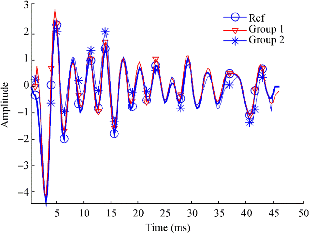Figure  1  Channel estimation results of the two groups

Download: Full-Size Img

The channel estimate at different SNR levels is depicted in Figure 2. The simulations show that group 1 outperforms group 2 in all cases. The estimation errors of both groups gradually decrease with the increase in the SNR level. The estimation error in group 1 decreases rapidly with the SNR level. Specifically, group 1 gains more than group 2 when the same SNR level increases. At low SNR, the estimation error is lower in group 1 than in group 2 by 0.1–0.5 dB, and the performance improvement is unnoticeable. When the SNR is greater than 25 dB, the estimation error is approximately 5 dB lower in group 1 than in group 2. Therefore, group 1 shows a significant advantage in the estimation error. When the SNR is greater than 70 dB, the estimation errors of groups 1 and 2 stabilize and remain nearly unchanged. At this point, the estimation error is lower by approximately 5 dB in group 1 than in group 2. The estimation error of group 2 fluctuates by approximately 2 dB as the SNR increases from 20 to 70 dB. Group 1 fluctuates between 40 and 60 dB with a fluctuation range of 1 dB. These features indicate that group 1 can achieve high-quality channel estimation.

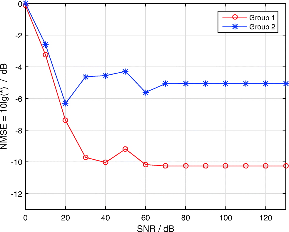Figure  2  Normalized mean square error (NMSE) of the channel estimation with different SNR levels

Download: Full-Size Img

Several different data lengths are demonstrated in Figure 3 to show their effect on the channel estimation errors. The estimation error does not monotonically change with the increase in the time length of the source signal, thus indicating that signal duration is another factor that affects the channel estimation, which is disregarded in the theoretical model of this study. Fundamentally, the signal described by Eq. (10) is an ideal model, and the signal time length that strictly conforms to the condition tends to infinity, which is infeasible in the real system. Figure 3 shows that the estimation error of group 1 decreases with the increase in the duration of the source signal. The curve of group 2 is opposite that of group 1. The simulation results show that group 1 outperforms group 2 in most cases. The estimation error is 1–4 dB lower in group 1 than in group 2. When the SNR increases to 60 dB, a significant difference can be observed in the estimation error between the two groups. The estimation error is more than 2 dB lower in group 1 than in group 2 in most cases and even reaches 10 dB, as shown in Figure 3b, when the duration of the source signal is 5 s. In Figsure 3 a and b, the estimation error of group 2 shows an upward trend when the duration of the source signal is greater than 3 s. The maximum estimation error also appears at an interval of 4–5 s. The estimation error of group 1 gradually decreases after 3 s. A long source signal duration may result in a high estimation error for group 2, but a low estimation error will be obtained for group 1.

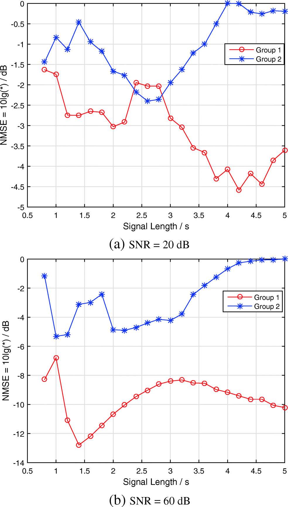Figure  3  NMSE of estimation given the different source lengths

Download: Full-Size Img

Although several methods for estimating the channel order exist (Karakutuk and Tuncer 2011), a particular channel order is difficult to estimate. An accurate length based on noisy and short data collection is difficult to determine. Figure 4 presents the relationship between the channel order and the estimation error for the SNR of 20 and 60 dB.

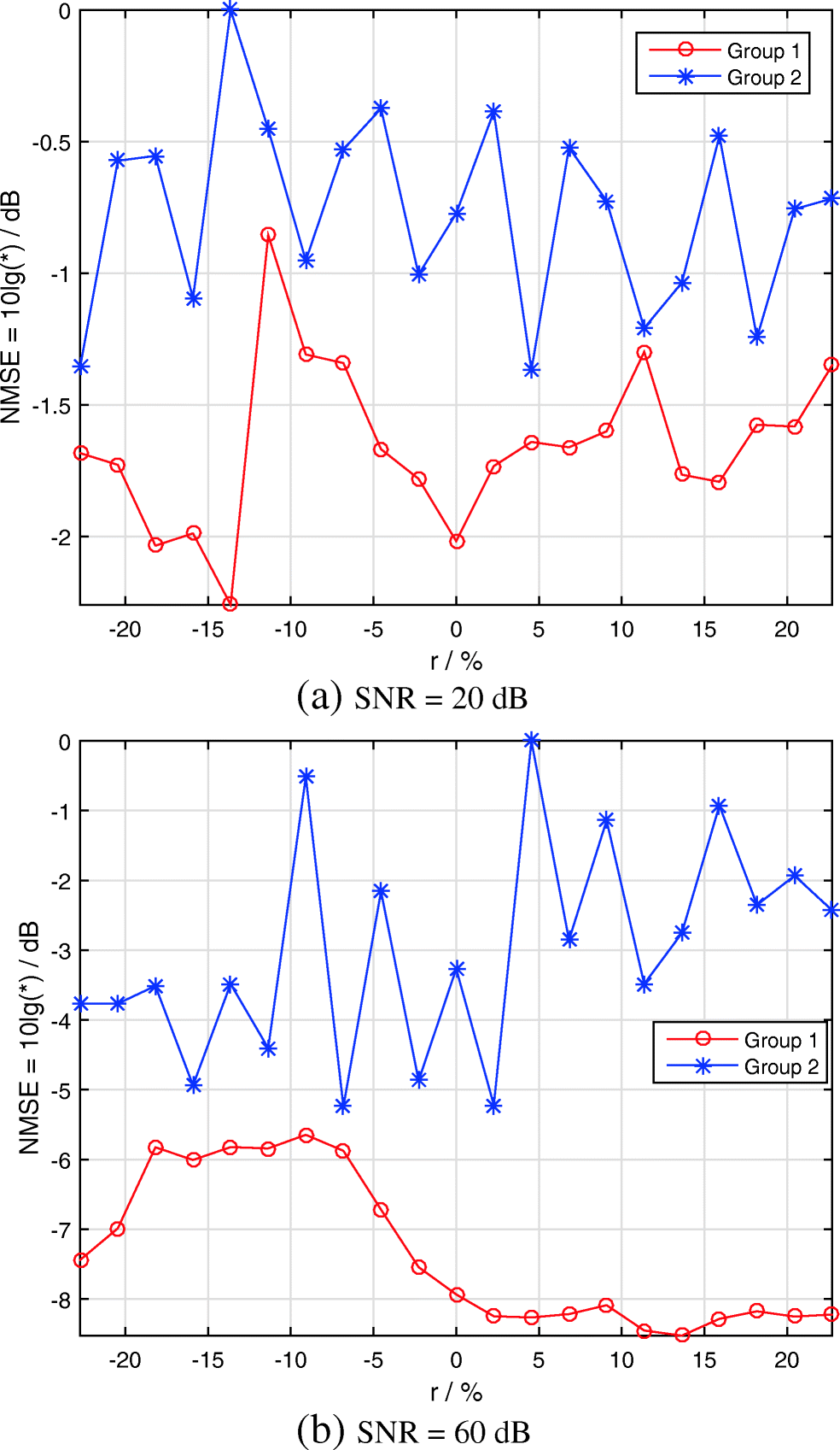Figure  4  NMSE of the channel estimate given channel length mismatch

Download: Full-Size Img

Considering that the same channel differs in terms of the numerical value of order in two groups, the ratio r of the difference between the estimated and the true orders is used as a criterion. r is defined as:

Figure 4 depicts the simulation results for the SNR of 20 and 60 dB. When the SNR is 20 dB, the channel estimation error of groups 1 and 2 is not significantly related to the channel estimation order. The estimation error is less than 1 dB lower in group 1 than in group 2, and the advantage is not evident. When the SNR is 60 dB, the estimation error of group 2 still has no evident relationship with the channel order, but group 1 shows a clear law. When −10 % < r < 0, a high error level in order estimation indicates a large channel estimation error. When 0 < r < 10%, the estimation error of group 2 still changes drastically with its increase, whereas that of group 1 stabilizes and remains at a lower level. The NMSE is 4–5 dB lower in group 1 than in group 2, thereby indicating that group 1 is not sensitive to overestimation of the channel order in the case of a high SNR. This feature provides a flexible selection for channel estimation at a high SNR. Specifically, when the SNR of the received data is relatively high, the channel order can be set to a higher value without substantially degrading the estimated quality. At this point, an accurate estimation of the channel order is unnecessary, and only a rough estimation is required.

Groups 1 and 2 are then run on the same computer, and the computation time is recorded. Figure 5a illustrates the relationship between computation time and signal length. Figure 5b depicts the relationship between computation time and channel length. In Figure 5a, the computation time increases linearly with the input signal length. Moreover, the computation time is much smaller in group 1 than in group 2. In Figure 5b, the computation time increases nonlinearly with the channel order. The computation time of group 2 increases rapidly with the channel length, whereas the computation time of group 1 increases slowly. This result occurred because the channel order in group 1 is a times that of group 2. Accordingly, the matrix dimension decomposed by the SVD is low. Therefore, group 1 consumes less time. Unlike the condition shown by the curves of group 2 in Figures 5 a and b, the computation time is sensitive to the channel order. Thus, the reduction in the channel order will decrease the computational time effectively. Table 2 lists the ratio of elapsed time between the two groups. The excellent acceleration performance of group 1 is shown. The computation time of group 2 is 10 to 40 times higher than that of group 1.

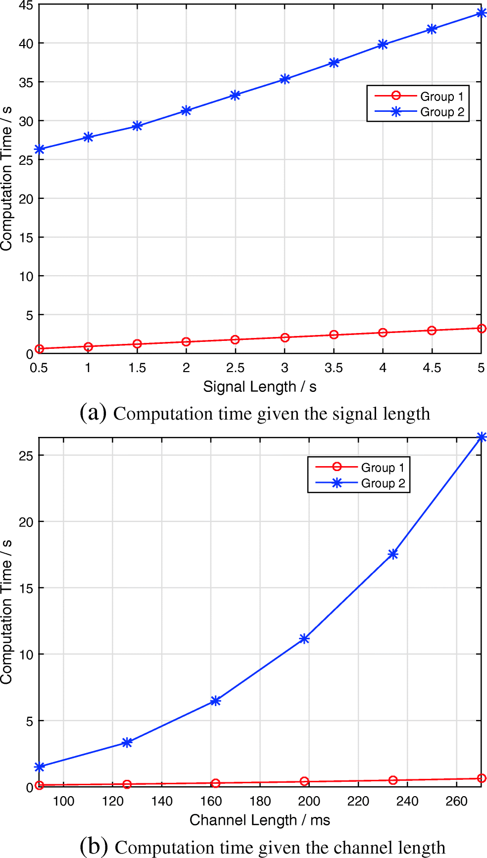Figure  5  Relationship between computation time and channel length

Download: Full-Size Img

5   Conclusions

Blind channel identification is crucial for many communication problems when the source signal is bandpass white. This study presents a frequency transformation-based approach that can enhance channel estimation by using the OPDA under the condition of a bandpass white source. This approach can be considered a generalized method for the OPDA because it extends the application of the algorithm from a white source to any bandpass white source or even the chirp signal. The modeling error of the covariance matrix is minimized by selecting proper parameters in the frequency transformation, thereby leading to a more accurate estimation by using the bandpass white source. The numerical simulation results verify that the proposed approach outperforms the raw OPDA in terms of NMSE. With the bandpass white source, the channel estimation error is reduced by approximately 5 dB at an SNR of 60 dB. In narrow-band systems, the proposed approach can effectively improve the computational speed of the algorithm. The new approach saved computational time by more than 90% in the simulations and can be easily incorporated into existing covariance-based algorithms.