-
Abstract
This paper aims to evaluate the feasibility of pressure-dependent models in the design of ship piping systems. For this purpose, a complex ship piping system is designed to operate in firefighting and bilge services through jet pumps. The system is solved as pressure-dependent model by the piping system analysis software EPANET and by a mathematical approach involving a piping network model. This results in a functional system that guarantees the recommendable ranges of hydraulic state variables (flow and pressure) and compliance with the rules of ship classification societies. Through this research, the suitability and viability of pressure-dependent models in the simulation of a ship piping system are proven.Article Highlights• In contrast to water distribution systems, in the naval sphere, the emitting components are usually known; therefore, pressure-dependent models are very viable.• Pressure-dependent models avoid the design of ship piping systems by means of arbitrary, intuitive, or conservative rules.• The relationships between pressure and flows in the emitting nodes are established, rather than predefining the demand of the system. -
1 Introduction
Ship piping systems (SPSs) are piping networks that intervene in most of a vessel's functions and might represent an important part of the cost and total weight of a vessel (Taylor 1996; Eyres and Bruce 2012; Asmara 2013). The design and production of these systems is considered by some specialists as one of the most complex tasks in shipbuilding (Cassee 1992; Li et al. 2010).
In the design phase of SPSs, predicting the distribution of flows and pressures in the network is often necessary and is achieved by solving a nonlinear equation system that constitutes the piping network model.
In demand-dependent models, pre-establishing the demand of the piping system (inflow or outflow) is necessary (Todini 2003; Elhay et al. 2015). This procedure can lead to mathematically correct solutions; however, the demand actually leaves the system through orifices, and flow is therefore determined by orifice opening (emitting node) and pressure (Walski et al. 2017). This fact has led to the development and increasing application of pressure-dependent models (PDMs), in which a relationship between the demand and pressure at the emitting nodes is established (Elhay et al. 2015). The most common flow-pressure relationship is based on the discharge of the flow through an orifice (Rossman 1994), as will be seen in Section 3.
PDMs are currently a subject of great interest in the field of water distribution systems (Tanyimboh et al. 2003; Sayyed et al. 2015; Walski et al. 2017). However, in this branch, controlling all domestic emitters is practically impossible; instead, each emitting node of the model constitutes a consumption area. In contrast, in the SPSs, there are generally well-defined emitting elements, such as open pipe exits, orifice exits, tank discharges, hose nozzles, hydro shields, sprinklers, injectors, and water/foam branchpipes.
In the naval sphere, special attention is given to the following: (ⅰ) to guarantee the recommended ranges of hydraulic state variables (flow and pressure), (ⅱ) to comply with the rules of ship classification societies, (ⅲ) to reduce the costs and weights of SPSs, and (ⅳ) to establish a better distribution of SPSs (Kang et al. 1999; Kim et al. 2013; Jiang et al. 2015; Molina et al. 2017). Then, pre-establishing the demands by arbitrary, intuitive, or conservative rules would make difficult the optimal design of the system based on the aspects mentioned below or, even worse, could result in a nonfunctional system.
In this work, a complex SPS is designed. It can operate in jet pumps used in the firefighting and bilge services. The system is solved as a PDM by the piping system analysis software EPANET (Rossman 1994) and by a mathematical approach based on a piping network model. This results in a functional system that also guarantees the recommended ranges of the flow variables and complies with the rules of the Ship Classification Society Bureau Veritas (2009). Through this research, the suitability and viability of the PDMs in the simulation of the SPSs are proven.
2 Design Aspects
To not divert attention from the main objective, only some considerations for the design of the fire protection and bilge system are mentioned below.
2.1 General Characteristics of the Ship
The characteristics of the ship are presented in Table 1.
Table 1 General characteristicsParameter Value Length (m) 35 Breadth (m) 10 Molded depth (m) 5 Maximum displacement (t) 160 2.2 Firefighting System
The addition of a manual control monitor branchpipe as part of the firefighting system is required. According to the manufacturer, the branchpipe operates in optimum conditions between 70 and 120 m of pressure head. It is recommended that the flow velocity in the system does not exceed 5 m/s, to avoid high head losses. Cavitation of the flow must be avoided.
According to the Bureau Veritas rules (2009), relief valves should be placed and adjusted in a way to prevent excessive pressure in any part of the fire main system.
2.3 Bilge System
The selected pump for the firefighting system should be used in the bilge of a compartment. In the same way, velocities higher than 5 m/s and cavitation of the flow must be avoided.
According to the Bureau Veritas rules (2009), each required bilge pump must have a capacity such that the velocity, in the main bilge pipe, whose diameter is calculated by Equation (1), must not be less than 2 m/s.
$$ d=25+1.68\sqrt{L\ \left(B+D\right)} $$ (1) where L, B, and D are the length, breadth, and molded depth, respectively, in m, and d is the internal diameter of the bilge main, in mm.
The internal diameter of pipes situated between the main bilge pipe and suction wells, in mm, is not to be less than the diameter, given by:
$$ {d}_1=25+2.16\sqrt{L_1\left(B+D\right)}\kern0.5em $$ (2) where L1 is the length of the compartment, in m.
3 Design and Simulation of the Firefighting and Bilge System
In the first instance, the system shown in Figure 1 is designed. It can be utilized in firefighting by opening the valves located in pipes 3 and 12 and closing the valves located in pipes 4 and 7, which allows the suctioning of water from the sea chests and discharging by the water branchpipe. In pipe 10, a relief valve is installed, which in case of excessive pressures releases flow through the open pipe exit in broadside (pipe 6).
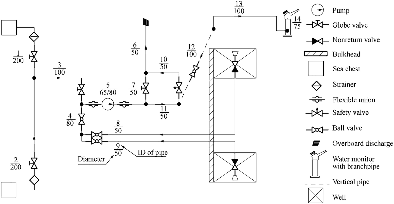 Figure 1 Principle diagram of firefighting and bilge system, diameter in millimeters
For the bilge service, the valves located in pipes 3 and 12 are closed, and the valves in pipes 4 and 7 are opened, which allows suctioning from the wells and discharging through pipe 6.
The pipe and node data of the piping system are shown in Table 2.
Table 2 Pipe and node data of the piping networkID of pipe L (m) D (mm) Kacc 1 4.0 200 5.24 2 4.0 200 5.24 3 0.5 100 6.09 4 Valve 80 7.08 5 Pump Pump Pump 6 2.0 50 1.14 7 Valve 50 7.64 8 11.5 50 1.92 9 12.0 50 1.92 10 0.5 50 12.00 11 0.5 100 0.38 12 7.5 100 0.59 13 4.6 100 0.81 14 Branchpipe 75 Branchpipe Notes: The total heads of the sea chests and wells are 1 m and 0 m, respectively. All nodes have 1 m of elevation, except the nodes that constitute pipe 13, with 8.5 m, as well as those that constitute the branchpipe and overboard discharge, with 10.1 m and 2 m, respectively. Through Equation (1), 63 mm of diameter is obtained for the main bilge pipe (pipe 4), transformed to 80 mm. According to Equation (2), the bilge branch diameter is 50 mm. The roughness coefficient of Willians Hazen is 125 (galvanized steel) (Sotelo 1982) The selected monitor is manually controlled, with 75 mm diameter (see Figure 2). Monitor performance is determined by the relationship between the flow and head loss in the monitor; this relationship is adjusted using Equation (3).
$$ hf=5544{Q}^2;{R}^2=0.9964 $$ (3) 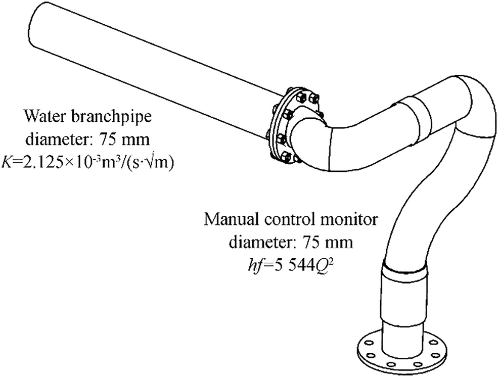 Figure 2 Manual control monitor branchpipe
where hf is the head loss in the monitor, in m; Q is the flow, in m3/s; and R2 is the determination coefficient, dimensionless.
As mentioned in the introduction, in this paper, we use the flow-pressure relationship based on the discharge of the flow through an orifice:
$$ {Q}_d=K\sqrt{P/\gamma } $$ (4) where K is the flow coefficient, in $ {\mathrm{m}}^3/\left(\mathrm{s}\cdotp \sqrt{\mathrm{m}}\right) $, which is usually determined by experiments for each emitting node; Qd is the demand, in m3/s; P is the pressure at the emitting node, in N/m2; and γ is the specific weight, in N/m3.
The selected branchpipe has 75 mm diameter (Figure 2), with a flow coefficient of 2.125 × 10⁻³$ {\mathrm{m}}^3/\left(\mathrm{s}\cdotp \sqrt{\mathrm{m}}\right) $ (127.71$ \mathrm{l}/\left(\min \cdotp \sqrt{\mathrm{m}}\right) $).
The selected centrifugal pump 65/260 at 2900 rpm is represented by plots of pressure head vs. flow (Figure 3) and the net positive suction head required (NPSHR) vs. flow (Figure 4).
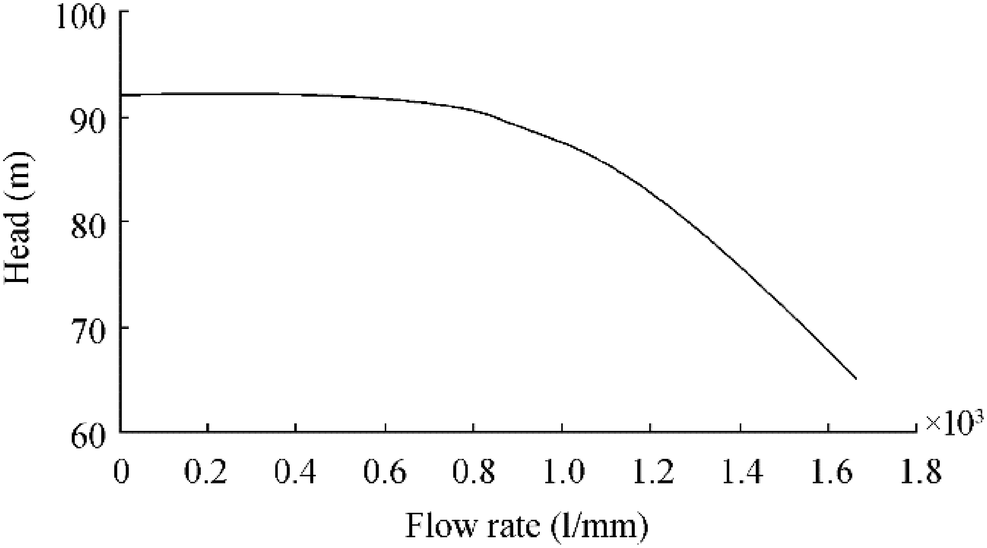 Figure 3 Pressure head vs. flow curve
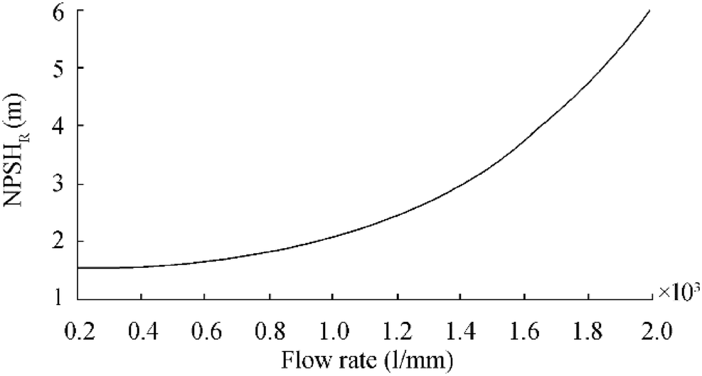 Figure 4 NPSHR vs. flow curve
To ensure that two systems operate in accordance with the requirements, both are simulated using EPANET (Rossman 1994).
As usual, the accessories (valves, elbows, strainers, and others) are introduced into the model by means of loss coefficients (Kacc) (Table 2). The monitor is represented by a general-purpose valve; through this valve, Eq. (3) is declared. The emitters, such as the branchpipe and open pipe exit in the broadside, are represented by flow coefficients (K).
The K of the open pipe exit, according to Molina et al. (2017), can be determined as shown in Equation (5).
$$ K=\sqrt{\frac{A^22g}{K_{\mathrm{acc}}}} $$ (5) where g is the gravity, in m/s2; A is the pipe section area, in m2; and Kacc = 1 (to open pipe exit). Considering that pipe 6 has 50 mm diameter, K = 8.7 × 10⁻³$ {\mathrm{m}}^3/\left(\mathrm{s}\cdotp \sqrt{\mathrm{m}}\right) $ (522$ \mathrm{l}/\left(\min \cdotp \sqrt{\mathrm{m}}\right) $).
3.1 Simulation Results
Figure 5 a and b show the results of firefighting and bilge system simulation using EPANET.
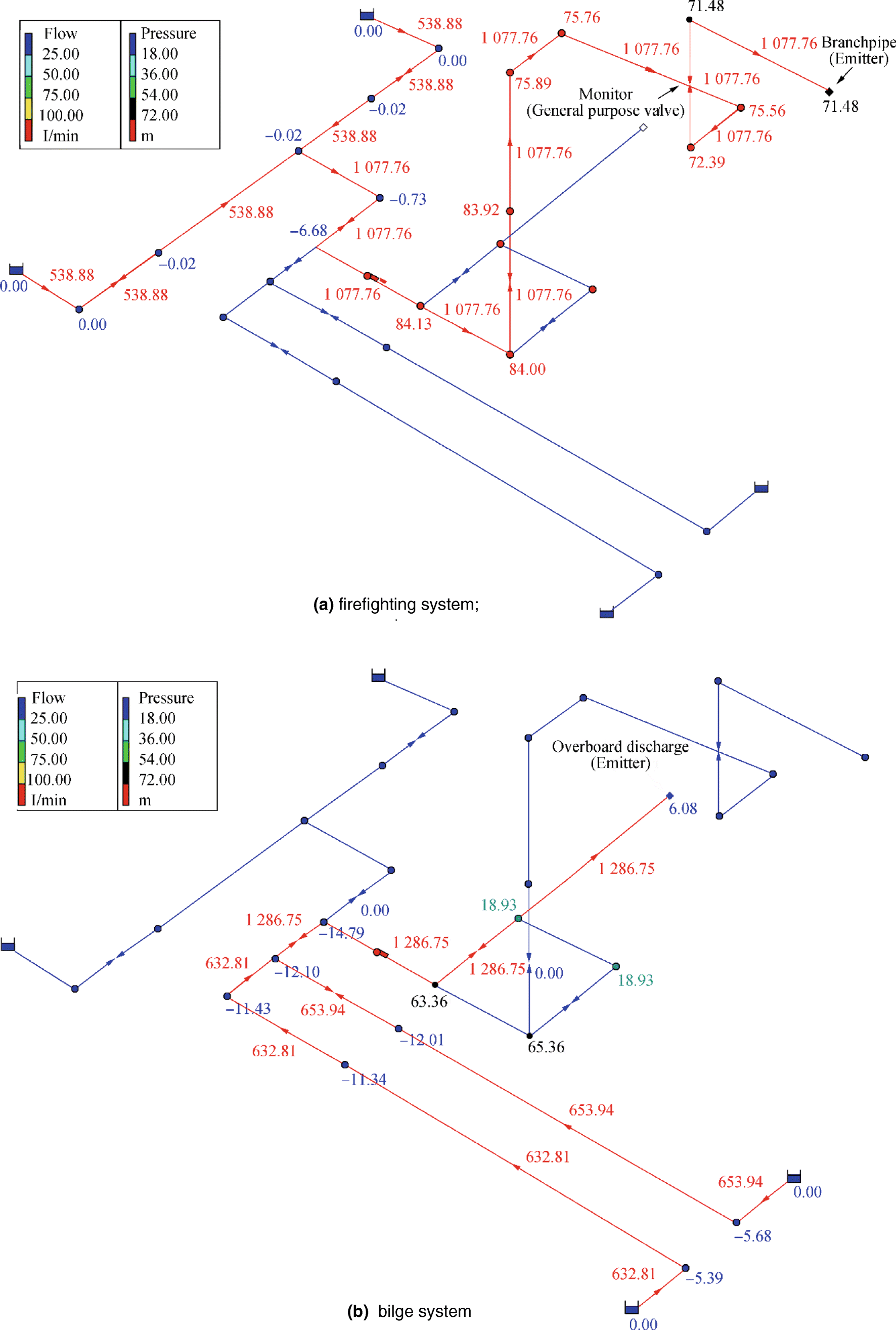 Figure 5 Modeling results
Then, in the firefighting system, the operating pump was 1.8 × 10⁻² m3/s (1078 l/min) and 85.81 m. As can be checked, the flow velocity did not exceed 5 m/s. At the inlet of the relief valve, there was 84 m of pressure head; then, the relief valve was preset at 93 m (10% of the working pressure). In the discharge of the branchpipe, there was 71.5 m, in accordance with the manufacturer's recommendations. According to Figure 4, the NPSHR (1078 l/min) ≈ 2.15 m, and the NPSHA is obtained as follows:
$$ {\mathrm{NPSH}}_{\mathrm{A}}\left(1078\frac{\mathrm{l}}{\min}\right)=\frac{P_{\mathrm{atm}}}{\gamma }-Z- hf-\frac{P_v}{\gamma }=8.41 $$ (6) where Patm is the atmospheric pressure, in N/m2; Z is the difference between the suction and eye of the pump, in m; and Pv is the vapor pressure of the water, in N/m2.
So that NPSHA > NPSHR and no cavitation occurs in the pump. Thus, requirements in the Section 2.2 are met. Note that in this system, the PDM expression is essential; otherwise, significant assumptions would be required to pre-establish the demand, resulting in uncertainties in each of the exposed requirements. In addition, it would make difficult the optimal design of the system taking into account costs, weights, and distribution; even worse, a nonfunctional system could result.
In the bilge system (Fig. 5b), the pressure head on the suction side of a pump was − 14.79 m, which indicates, without the need to analyze the NPSH, that cavitation occurs, because the value is even below that of the absolute zero pressure. This pressure, although impossible in reality, solves the system, and it is due mainly to the following: (ⅰ) the system has a large part of its design in the suction side of the pump, while in the discharge side, there is practically no resistance; (ⅱ) the pump is oversized to operate in this system. Both reasons lead to an inadmissible pressure gradient.
To utilize a firefighting pump in the bilge service, the use of jet pumps is an alternative, which is mentioned in the Bureau Veritas rules (2009). In this variant, the firefighting pump drives water from the sea chests to the jet pumps. In the jet pumps, a sub-atmospheric pressure that allows to suction water from the wells is generated, to subsequently discharge the water into the sea. According to Katen (2007), firefighting pumps are usually used in bilge systems with jet pumps, due to the high pressures required.
In Figure 6 and Table 3, the design of the bilge system with jet pumps is shown. One jet pump is conceived for each well. Note that the flows arrive to jet pumps via pipes 8 (main flow 1) and 9 (main flow 2). These flows should produce the sufficient sub-atmospheric pressure to suction flow through pipes 6 (secondary flow 1) and 7 (flow secondary 2). According to the Bureau Veritas rules (2009), the traditional bilge system must guarantee at least 2 m/s in the main bilge pipe (with a diameter of 60 mm), which is equivalent to 5.7 × 10⁻³m3/s (339 l/min). To maintain that evacuation capacity, the sum of the two secondary flows must not be less than 5.7 × 10⁻³m3/s.
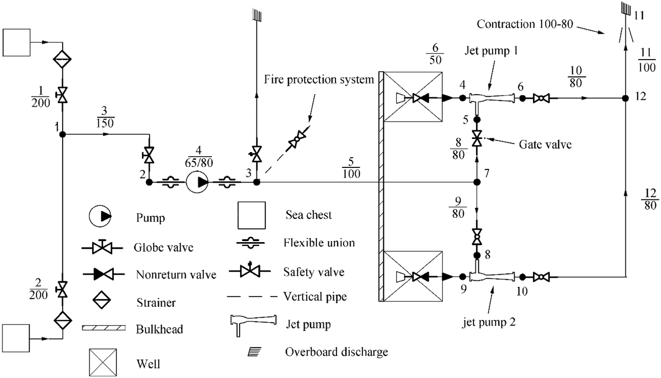 Figure 6 Principle diagram of the bilge system with jet pumps, diameter in millimetersTable 3 Pipe and node data of piping system
ID of pipe L (m) D (mm) Kacc 1 4.0 200 5.24 2 4.0 200 5.24 3 0.5 150 7.36 4 Pump Pump Pump 5 8.0 100 1.02 6 0.5 50 1.86 7 0.5 50 1.86 8 2.5 80 15.08 9 2.5 80 1.13 10 1.0 80 1.13 11 2.0 100 1.42 12 6.0 80 0.94 Notes: The total head of the sea chests and wells are 1 m and 0 m, respectively. All nodes have 1 m of elevation, except those of the overboard discharge with 2 m. Manning's roughness coefficient is 0.011 (smooth steel) (Walski et al. 2003) Unfortunately, EPANET does not have the capacity to include jet pumps, and programs that allow the simulation of jet pumps as part of a piping network are unknown. Then, for modeling the bilge system with jet pumps, employing the mathematical model is necessary.
3.2 Mathematical Model of the Bilge System with Jet Pumps
Numerous studies, such as Fuertes et al. (2002) and Boulos et al. (2006), describe in detail the different piping network models. In this section, a piping network model with node equation formulation is employed, since few equations are required to define the networks.
3.2.1 Piping Network Model with Node Equations Formulation
The model is a system of nonlinear equations with total head unknowns, resulting from the conservation equations of mass at nodes in terms of nodal heads (Boulos et al. 2006). Expressing the head loss equation in a generic form results in:
$$ {H}_j-{H}_i=r{Q}^n+\frac{K_{\mathrm{acc}}}{A^22g}{Q}^2 $$ (7) where Hj and Hi are the total heads at nodes j and i, respectively, in m; the first term on the right-hand side is associated with the head losses in the straight pipes; r and n depend on the loss equation selected. The second term is associated with the losses in accessories.
If the Manning equation is used, then Equation (7) can be expressed as:
$$ {H}_j-{H}_i=\left(\frac{10.29L{n}^2}{D^{5.33}}+\frac{K_{\mathrm{acc}}}{A^22g}\right){Q}^2 $$ (8) where L is the length of pipe, in m; n is Manning's roughness coefficient, dimensionless; and D is the pipe diameter, in m. Isolating Q in Equation (8) and replacing in the conservation equation of mass results in Equation (9), which is the fundamental equation in this model.
$$ \sum \limits_{l=1}^{J_{\mathrm{in},\mathrm{i}}}{\alpha}_l{\left(H-{H}_i\right)}^{1/2}-\sum \limits_{l=1}^{J_{\mathrm{out},\mathrm{i}}}{\alpha}_l{\left({H}_i-H\right)}^{1/2}={q}_i $$ (9) with:
$$ {\alpha}_l={\left(\frac{10.29L{n}^2}{D^{5.33}}+\frac{K_{acc}}{A^22g}\right)}^{-1/2} $$ (10) where qi is the demand at node i, in m3/s; Jin, i and Jout, i are the numbers of the inflow pipes and outflow pipes respect to node i; and H is the node head that jointly with Hi constitutes the pipe l.
Equation (11) is a power curve fitting of the centrifugal pump curve of Figure 3 (Q in m3/s). Similarly, the flow of (11) is isolated and incorporated in (9) for the nodes connected to the pump.
$$ H=92-3.817\times {10}^{6}\ast {Q}^{3.302};{R}^2=0.996 $$ (11) 3.2.2 Jet Pump Model
Elger et al. (1991) developed a model used to simulate jet pumps in networks. The model is composed of the empirical curves f1 and f2, which are dependent on the flow fraction Qs/Qd (Figure 7). The product of these two curves with the velocity head in the discharge of the jet pump (point 4, Figure 7) determines the head losses between 1 and 4 as well as 2 and 4. Applying the conservation of energy and mass in jet pumps results in:
$$ {H}_1-{H}_4={f}_1\left(\frac{Q_s}{Q_d}\right)\ast \frac{V_4^2}{2g}\equiv {f}_1\left(\frac{Q_s}{Q_d}\right)\ast \frac{Q_d^2}{2g{A_4}^2}\kern0.5em $$ (12) $$ {H}_2-{H}_4={f}_2\left(\frac{Q_s}{Q_d}\right)\ast \frac{V_4^2}{2g}\equiv {f}_2\left(\frac{Q_s}{Q_d}\right)\ast \frac{Q_d^2}{2g{A_4}^2} $$ (13) $$ {Q}_m+{Q}_s-{Q}_d=0 $$ (14) 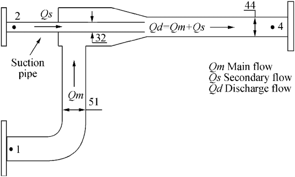 Figure 7 Annular jet pump geometry, dimensions in millimeters
The use of the annular jet pump presented by Elger et al. (1991) is proposed, and its geometry is shown in Figure 7.
Equations (15) and (16) are polynomial fittings of the experimental curves f1 and f2, with determination coefficients of 0.9995 and 0.9997, respectively. However, the flows of Equations (15) and (16) cannot be isolated; then, the jet pumps cannot be expressed in terms of nodal heads, but through Equations (12)-(14).
$$ {f}_1\left(\frac{Q_s}{Q_d}\right)=1.35{\left(\frac{Q_s}{Q_d}\right)}^2-10.65\frac{Q_s}{Q_d}+6.48 $$ (15) $$ {f}_2\left(\frac{Q_s}{Q_d}\right)=-3.63{\left(\frac{Q_s}{Q_d}\right)}^2+10.46\frac{Q_s}{Q_d}-3.86 $$ (16) 3.2.3 Mathematical Model for the Bilge System with Jet Pumps
Equation (9) is applied to each node of the bilge system, resulting in Equations (17)-(34). See that Equations. (18) and (19) correspond to nodes 2 and 3, which contain the pump equation. The open pipe exit to the atmosphere is represented in Equation (27), and it establishes the PDM. Equations (29)-(34) correspond to the jet pumps, with the flow as unknowns, as explained above. Then, 18 equations with 18 unknowns are obtained.
$$ {\alpha}_1{\left({H}_{sc}-{H}_1\right)}^{1/2}+{\alpha}_2{\left({H}_{sc}-{H}_1\right)}^{1/2}-{\alpha}_3{\left({H}_1-{H}_2\right)}^{\frac{1}{2}}=0 $$ (17) $$ {\alpha}_3{\left({H}_1-{H}_2\right)}^{1/2}-{\left(\frac{H_3-{H}_2-92}{-3.817\times {10}^6}\right)}^{1/3.302}=0 $$ (18) $$ {\left(\frac{H_3-{H}_2-92}{-3.817\times {10}^6}\right)}^{1/3.302}-{\alpha}_5{\left({H}_3-{H}_7\right)}^{1/2}=0 $$ (19) $$ {\alpha}_6{\left({H}_w-{H}_4\right)}^{1/2}-{Q}_{s1}=0 $$ (20) $$ {\alpha}_8{\left({H}_7-{H}_5\right)}^{1/2}-{Q}_{m1}=0 $$ (21) $$ {Q}_{d1}-{\alpha}_{10}{\left({H}_6-{H}_{12}\right)}^{1/2}=0 $$ (22) $$ {\alpha}_5{\left({H}_3-{H}_7\right)}^{1/2}-{\alpha}_8{\left({H}_7-{H}_5\right)}^{\frac{1}{2}}-{\alpha}_9{\left({H}_7-{H}_8\right)}^{\frac{1}{2}}=0 $$ (23) $$ {\alpha}_9{\left({H}_7-{H}_8\right)}^{1/2}-{Q}_{m2}=0 $$ (24) $$ {\alpha}_7{\left({H}_w-{H}_9\right)}^{1/2}-{Q}_{s2}=0 $$ (25) $$ {Q}_{d2}-{\alpha}_{12}{\left({H}_{10}-{H}_{12}\right)}^{1/2}=0 $$ (26) $$ {\alpha}_{11}{\left({H}_{12}-{H}_{11}\right)}^{1/2}-K{\left({H}_{11}-{Z}_{11}\right)}^{1/2}=0 $$ (27) $$ {\alpha}_{12}{\left({H}_{10}-{H}_{12}\right)}^{1/2}-{\alpha}_{11}{\left({H}_{12}-{H}_{11}\right)}^{\frac{1}{2}}+{\alpha}_{10}{\left({H}_6-{H}_{12}\right)}^{\frac{1}{2}} \\ \ \ \ \ \ =0 $$ (28) $$ {Q}_{m1}+{Q}_{s1}-{Q}_{d1}=0 $$ (29) $$ {Q}_{m2}+{Q}_{s2}-{Q}_{d2}=0 $$ (30) $$ {H}_4-{H}_6-{f}_2\left(\frac{Q_{s1}}{Q_{d1}}\right)\ast \frac{{Q_{d1}}^2}{2g{A_4}^2}=0 $$ (31) $$ {H}_5-{H}_6-{f}_1\left(\frac{Q_{s1}}{Q_{d1}}\right)\ast \frac{{Q_{d1}}^2}{2g{A_4}^2}=0 $$ (32) $$ {H}_9-{H}_{10}-{f}_2\left(\frac{Q_{s2}}{Q_{d2}}\right)\ast \frac{{Q_{d2}}^2}{2g{A_4}^2}=0 $$ (33) $$ {H}_8-{H}_{10}-{f}_1\left(\frac{Q_{s2}}{Q_{d2}}\right)\ast \frac{{Q_{d2}}^2}{2g{A_4}^2}=0 $$ (34) where Hsc and Hw are the total head of the sea chests and wells, respectively. Qm1, Qs1, and Qd1 are the main flow, secondary flow, and discharge flow of jet pump 1, respectively. Moreover, Qm2, Qs2, and Qd2 are the main flow, secondary flow, and discharge flow of jet pump 2, respectively, and K is the flow coefficient of the open pipe exit ($ 2.2\times {10}^{-2}{\mathrm{m}}^3/\left(\mathrm{s}\cdotp \sqrt{\mathrm{m}}\right) $).
3.2.4 Solution of the Bilge System with Jet Pumps
The system of nonlinear equations is solved by the Levenberg-Marquardt algorithm (More 1977). The solution was found in iteration 230, with the value of the objective function (function tolerance) less than 1 × 10⁻¹⁰.
The results are shown in Figure 8. Because jet pump 2 has a greater resistance downstream (pipe 12) than jet pump 1 (pipe 10), the flow to jet pump 1 was significantly higher. Then, the gate valve of pipe 8 was regulated to an opening of 30% to balance the flows.
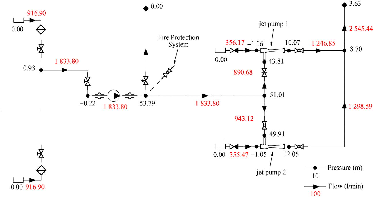 Figure 8 Modeling results of the bilge system with jet pumps
Notice that the pump operated at 3.14 × 10⁻² m3/s (1883.80 l/min) and 54.01 m, except in pipe 11 where 5 m/s, was reached, and the flow velocity was kept lower than this value.
According to Figure 4, the NPSHR(1883.80l/min) ≈ 5.14m, and the NPSHA(1883.80 l/min) = 8.87m, so that NPSHA > NPSHR and no cavitation occurs in the pump. The sum of the secondary flows of the jet pumps was 1.19 × 10⁻² m3/s (711.64 l/min), higher than the flow required by the rules (339 l/min). According to Winoto et al. (2000), the efficiency of jet pumps is defined as:
$$ \eta =\frac{Q_s}{Q_m}\ast \frac{H_4-{H}_2}{H_1-{H}_4} $$ (35) Then, the efficiency of the jet pumps was about 13%, which is a typical efficiency for jet pumps, according to a study of commercial jet pump efficiency developed by Manzano (2008), although some authors have achieved efficiencies up to 45% (Feitosa et al. 1997). Thus, the exposed requirements in Section 2.3 were met.
As in the previous case, in this system, the expression of the PDM is fundamental. Consider the complexity of predefining the demand for a system with jet pumps in parallel, that is, to establish a demand-dependent model. In Section 3.1, the possible problems of a wrongly pre-established demand are mentioned. In addition, the erroneous operation of the jet pumps would prevent the bilge or allow the entry of water into the ship (reverse flow) in the case that the non-return valve fails.
4 Conclusions
In this work, the suitability of PDMs in the simulation of SPSs is demonstrated, since the relationships between pressure and flows in the emitting nodes are established, rather than predefining the demand of the system by means of arbitrary, intuitive, or conservative rules. In this way, PDMs contribute effectively to guarantee the systems functionality, the recommendable ranges of hydraulic state variables (flow and pressure), and compliance with the rules of ship classification societies.
In water distribution systems, where PDMs are widely applied, controlling all domestic emitters in the model is practically impossible; instead, each emitting node constitutes a consumption area, for which the relationships between flow and pressure must be determined. In contrast, this case study proves the viability of PDMs in the naval sphere, where the emitting components are usually known, as well as the relationships between the flow and the pressure of each emitting component.
Open Access This article is licensed under a Creative Commons Attribution 4.0 International License, which permits use, sharing, adaptation, distribution and reproduction in any medium or format, as long as you give appropriate credit to the original author(s) and the source, provide a link to the Creative Commons licence, and indicate if changes were made. The images or other third party material in this article are included in the article's Creative Commons licence, unless indicated otherwise in a credit line to the material. If material is not included in the article's Creative Commons licence and your intended use is not permitted by statutory regulation or exceeds the permitted use, you will need to obtain permission directly from the copyright holder. To view a copy of this licence, visit http://creativecommons.org/licenses/by/4.0/. -
Figure 1 Principle diagram of firefighting and bilge system, diameter in millimeters
Figure 2 Manual control monitor branchpipe
Figure 3 Pressure head vs. flow curve
Figure 4 NPSHR vs. flow curve
Figure 5 Modeling results
Figure 6 Principle diagram of the bilge system with jet pumps, diameter in millimeters
Figure 7 Annular jet pump geometry, dimensions in millimeters
Figure 8 Modeling results of the bilge system with jet pumps
Table 1 General characteristics
Parameter Value Length (m) 35 Breadth (m) 10 Molded depth (m) 5 Maximum displacement (t) 160 Table 2 Pipe and node data of the piping network
ID of pipe L (m) D (mm) Kacc 1 4.0 200 5.24 2 4.0 200 5.24 3 0.5 100 6.09 4 Valve 80 7.08 5 Pump Pump Pump 6 2.0 50 1.14 7 Valve 50 7.64 8 11.5 50 1.92 9 12.0 50 1.92 10 0.5 50 12.00 11 0.5 100 0.38 12 7.5 100 0.59 13 4.6 100 0.81 14 Branchpipe 75 Branchpipe Notes: The total heads of the sea chests and wells are 1 m and 0 m, respectively. All nodes have 1 m of elevation, except the nodes that constitute pipe 13, with 8.5 m, as well as those that constitute the branchpipe and overboard discharge, with 10.1 m and 2 m, respectively. Through Equation (1), 63 mm of diameter is obtained for the main bilge pipe (pipe 4), transformed to 80 mm. According to Equation (2), the bilge branch diameter is 50 mm. The roughness coefficient of Willians Hazen is 125 (galvanized steel) (Sotelo 1982) Table 3 Pipe and node data of piping system
ID of pipe L (m) D (mm) Kacc 1 4.0 200 5.24 2 4.0 200 5.24 3 0.5 150 7.36 4 Pump Pump Pump 5 8.0 100 1.02 6 0.5 50 1.86 7 0.5 50 1.86 8 2.5 80 15.08 9 2.5 80 1.13 10 1.0 80 1.13 11 2.0 100 1.42 12 6.0 80 0.94 Notes: The total head of the sea chests and wells are 1 m and 0 m, respectively. All nodes have 1 m of elevation, except those of the overboard discharge with 2 m. Manning's roughness coefficient is 0.011 (smooth steel) (Walski et al. 2003) -
Asmara A (2013) Pipe routing framework for detailed ship design. Association for Studies and Student Interest in Delft, Nederland, pp 1–11 Boulos PF, Lansey KE, Karney BW (2006) Comprehensive water distribution systems analysis handbook for engineers and planners. MWH Soft, Pasadena Bureau Veritas (2009) Rules for the classification of ships-part C: machinery, electricity, automation and fire protection. Neuilly-sur-Seine Cassee HJ (1992) Piping systems. In: Harrington RL (ed) Marine engineering. Society of Naval Architects and Marine Engineers, Jersey City, pp 782–845 Elger DF, Mclam ET, Taylor SJ (1991) A new way to represent jet pump performance. J Fluids Eng 113(3): 439–444. https://doi.org/10.1115/1.2909515 Elhay S, Piller O, Deuerlein J, Simpson A (2015) A robust, rapidly convergent method that solves the water distribution equations for pressure-dependent models. J Water Resour Plan Manag 142(2): 1–11. https://doi.org/10.1061/(ASCE)WR.1943-5452.0000578 Eyres DJ, Bruce GJ (2012) Pumping and piping arrangements. In: Eyres DJ, Bruce GJ (eds) Ship construction. Butterworth-Heinemann, Oxford, pp 315–325 Feitosa JC, Botrel TA, Pinto JM (1997) Strategies to improve the performance of the operational limit of Venturi-type injectors. I Iberian Congress and Ⅲ National Fertigation Congress (I Congreso Ibérico y Ⅲ Congreso Nacional de Fertirrigación). Murcia, Spain, pp 446–449. (in Portuguese) Fuertes VS, García-Serra J, Iglesia PL, López G, Martínez FJ, Pérez R (2002) Modeling and design of water supply networks. Polytechnic University of Valencia (Universidad Politécnica de Valencia), Spain ISBN: 84-89487-06-5. (in Spanish) Jiang WY, Lin Y, Chen M, Yu YY (2015) A co-evolutionary improved multi-ant colony optimization for ship multiple and branch pipe route design. Ocean Eng 102: 63–70. https://doi.org/10.1016/j.oceaneng.2015.04.028 Kang SS, Sehyun M, Hah SH (1999) A design expert system for auto-routing of ship pipes. J Ship Prod 15(1): 1–9. https://doi.org/10.2478/IJNAOE-2013-0146 Katen JH (2007) Engine room. In: Dokkum KV (ed) Ship knowledge. Ship design, construction and operation. Dokmar Maritime, Vlissingen, pp 236–261 Kim SH, Ruy WS, Seon B (2013) The development of a practical pipe auto-routing system in a shipbuilding CAD environment using network optimization. Int J Naval Arch Ocean Eng 5(3): 468–477. https://doi.org/10.2478/IJNAOE-2013-0146 Li R, Liu Y-J, Hamada K (2010) Research on the ITOC based scheduling system. J Mar Sci Appl 9(4): 355–362. https://doi.org/10.1007/s11804-010-1020-7 Manzano J (2008) Analysis of the venturi injector and improvement of the installation in the localized irrigation systems. Ph. D, thesis. Polytechnic University of Valencia (Universidad Politécnica de Valencia), Spain, 56-61. (in Spanish) Molina D, Quesada A, Febles Y, Ramos LC (2017) The computational simulation in the design of ship piping systems. J Hydraul Environ Eng 38(2): 29–43 ISSN: 1815-591X (in Spanish) More JJ (1977) The Levenberg-Marquardt algorithm: implementation and theory. U. S Department of Energy Office of Scientific and Technical Information. Available from www.osti.gov/servlets/purl/7256021 [accessed on July. 7, 2019] Rossman LA (1994) EPANET 2.0. EPANET users manual drinking water research division, risk reduction engineering laboratory, Office of Research and Development. U.S. Environmental Protection Agency, Cincinnaty Sayyed MAHA, Gupta R, Tanyimboh TT (2015) Noniterative application of EPANET for pressure dependent modelling of water distribution systems. Water Resour Manag 29(9): 3227–3242. https://doi.org/10.1007/s11269-015-0992-0 Sotelo G (1982) General hydraulic vol 1. Principles. Limusa, Mexico City, 294–295. (in Spanish) Tanyimboh T, Tahar B, Templeman A (2003) Pressure-driven modelling of water distribution systems. Water Sci Technol Water Supply 3(1-2): 255–261. https://doi.org/10.2166/ws.2003.0112 Taylor DA (1996) Introduction to marine engineering. Butterworth-Heinemann, Oxford, pp 112–134 Todini E (2003) A more realistic approach to the extended period simulation of water distribution networks. Proc. International Conference on Computing and Control for the Water Industry. Swets and Zeillinger, Lisse, Nederland, pp 173–213. https://doi.org/10.1201/NOE9058096081.ch19 Walski TM, Chase DV, Savic DA, Grayman W, Beckwith S, Koelle E (2003) Advanced water distribution modeling and management. Haestead Press, Waterbury, pp 30–38 ISBN: 0-9714141-2-2 Walski TM, Blakley D, Evans M, Whitman B (2017) Verifying pressure dependent demand modeling. Procedia Eng 186:364–371. https://doi.org/10.1016/j.proeng.2017.03.230 Winoto SH, Li H, Shah DA (2000) Efficiency of jet pumps. J Hydraul Eng 126(2): 150–156. https://doi.org/10.1061/(ASCE)0733-9429(2000)126%3A2(150)
| Citation: |
Daniel Molina Pérez, Lemuel C. Ramos-Arzola, Amadelis Quesada Torres (2020). Pressure-Dependent Models in Ship Piping Systems. Journal of Marine Science and Application, 19(2): 266-274. https://doi.org/10.1007/s11804-020-00146-2

|