1   Introduction

Environmental and economic factors, together with higher efficiency and reliability, drive the research for improved marine power generation. Marine systems could benefit greatly from the adoption of electrical drives on power systems in replacement of fossil-fuelled engines. Hydrogen is considered a valuable option and a good alternative to traditional fossil fuel resources, with fuel cells being a mature technology and used in many specific areas (Amamou et al. 2016). Fuel cells are modular by nature which gives an additional degree of freedom in the system design while their high efficiency leads to a more flexible fuel usage improving the overall autonomy. On the other hand, as with land-based transportation systems, technical barriers related to size, volume, thermal control, system complexity, etc. still need to be addressed satisfactorily. Among the currently available fuel cell technologies, proton exchange membrane fuel cells (PEMFC) are considered one of the most promising options for marine applications (Table 1) for low to intermediate power levels (up to 50 kW) combining high efficiency, rapid start-up and quick response to load changes.

Fuel cells produce electrical current by reversing the electrolysis process. The output voltage heavily depends on the operating conditions and hence comes with variable amplitude (Larminie and Dicks 2003a, b). Therefore, most fuel cells need to be interfaced with power loads by means of voltage regulators. Conditioning of the converter output is not trivial due to nonlinearities and discontinuities. DC regulators use a pulse-width modulation (PWM) signal to generate the output signal. Different methods exist in literature to control the power output of a switching converter. In this study, an artificial neural network (ANN) scheme is investigated (Cheng et al. 2016).

For the scope of this works, a PEMFC is interfaced with a resistive load (or consumer) using a DC voltage regulator.

Figure 1 shows a typical example of a fuel cell, power converter and load configuration.

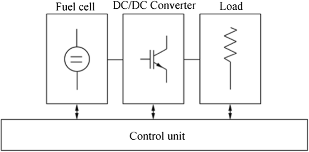Figure  1  Schematic of the proposed system

Download: Full-Size Img

1.1   Literature Review

Broadly speaking, fuel cells are mainly modelled using three approaches: analytical (or chemical), electrical and empirical. Analytical modelling is founded on the electrochemical reactions governing the fuel cell. It is widely used despite its limitations with respect to computation time and input parameters.

This type of model requires detailed and in-deep knowledge of the geometrical characteristics of the device such as transfer coefficients, internal humidity level and catalyst and layer thickness. Hence, they are suitable for electrochemical analysis and fine tuning of the aforementioned parameters (Chwei-Sen et al. 2000; Gebreselassie, 1994; Boscaino et al. 2013; Genduso and Miceli 2011; Hongtan and Zhou 2003; OHayre et al. 2016; Qiuli et al. 2006; Min Joong et al. 2005).

In power management applications, the behaviour of the fuel cell is embedded in a broader system. Therefore, equivalent circuit models are adopted where the fuel cell is represented by electrical circuit elements (Larminie and Dicks 2003a, b; Runtz and Lyster 2005). In empirical modelling, the electrochemical device is treated as a black box. The accuracy of this modelling technique, since mostly based on data fitting, depends on measurement performance, data filtering, modelling techniques, etc. (Chakraborty et al. 2012; Haji 2011; Bonanno et al. 2010; Di Dio et al. 2008; Ramos-Paja et al. 2010; Boscaino et al. 2008a, b; Boscaino et al. 2010; Barelli et al. 2011). Only few ANN implementations are found in literature (Kong and Khambadkone 2009; Tremblay et al. 2009). In this work, two different implementations of the same fuel cell are attempted. First, a model based on the one described in (Tremblay et al. 2009) is developed which combines the features of chemical, empiric and electrical models. In the second part of the manuscript, a self-learning, featuring fast-implementation ANN analogue of a fuel cell is presented.

Modelling of DC-DC converters, as found in literature, in mainly based on two techniques: the state-space averaging method and the circuit-averaging method (Maksimovic et al. 2001; Girish and Mohan 2001; Ben-Yaakov and Adar 1994; Kovar et al. 2009; Ren et al. 2000; Liu and Sen 1994; Wu and Chen 1998; Davoudi and Jatskevich 2006; Davoudi et al. 2006; Yang et al. 2012; Mahmood and Natarajan 2008; Galotto et al. 2009; Gatto et al. 2010; Gong et al. 2010; Gorecki and Zarebski 2006). These methods do not account for system non-idealities arising mostly from the semiconductor devices and parasitic components (Taghvaee et al. 2013). In this work, a state-space modelling approach using a dynamic simulator software (Matlab) is adopted in order to address two tasks: controlling the dynamics of the power converter and collect training data for a later ANN cycle-to-cycle equivalent, with this last point which is among the novelties of this work.

Controlling of switching DC-DC converters is achieved using different methods: digital control methods (Feng et al. 2007; Corradini et al. 2009), traditional PI and PID controllers, FIR (finite impulse response) filter method and IIR (infinite impulse response) (Kurokawa et al. 2010a, b; Kurokawa et al. 2011). However, a prediction based method, such an ANN approach, has been presented with very satisfactory results (Bishop, 2006; Kurokawa et al. 2010a, b). Drawing upon these results, a similar approach is attempted in this work.

1.2   Marine Application for Fuel Cell Technology

A concise example of the applicability of fuel cell technology to marine applications is electric propulsion unmanned vehicles using PMDC and waterjet (Xiros et al. 2009). Fuel cells are capable of enabling dc motors used to produce thrust for unmanned surface boats. Adaptive and efficient control by means of artificial neural networks of both the fuel cell and conditioning units permits efficient power management of the system minimizing the risk of propulsion power loss while the vessel is operating.

A second example involving an energy-harvesting application can be found in (Tsakyridis et al. 2016). Kinetic energy of moving water masses is harvest using underwater or tidal turbines and it has been later converted into chemical by electrolyzing units. The hydrogen produced is then available to both external users and to the systems' fuel cell units. The control scheme proposed in this work fully describes the fuel cell operation used to sustain autonomous operations of the power harvesting architecture.

Moreover, fuel cell technology may be suitable for marine vehicles with intelligent control (Wang et al. 2019a, b).

Finally, an overview of the most noticeable maritime fuel cell application research projects is given below (van Biert et al. 2016):

• Class 212, 1980–1998, Howaldtswerke-Deutsche Werft (Sattler 2000; McConnell 2010)

• SSFC, 1997–2003, Office of Naval Research (Allen et al. 1998; Privette et al. 2002; Bourne et al. 2001)

• DESIRE, 2001–2004, Naval Ship, Energy Research Centre Nld (Krummrich et al. 2006)

• FCSHIP, 2002–2004, Norwegian Shipowners' Association (Alkaner and Zhou 2006)

• FellowSHIP, 2003–2013, DNV Research and Innovation (Ludvigsen and Ovrum 2012; Fuel Cells Bull 2012)

• FELICITAS, 2005–2008, Frauenhofer Institute (Tse et al. 2011)

• MC-WAP, 2005–2011, CATENA (Specchia et al. 2008; Bensaid et al. 2009)

• ZEMSHIP, 2006–2010, ATG Alster Touristik Gmbh (Schneider et al. 2010; Vogler)

• METHAPU, 2006–2009, Wartsila Corporation (Díaz-de Baldasano et al. 2014; Strazza et al. 2010)

• Nemo H2, 2008–2011, Fuel Cell Boat BV (McConnell 2010)

• SchIBZ, 2009–2016, ThyssenKrupp marine systems (Leites et al. 2012; M.C. Díaz-de Baldasano et al. 2014)

• PaXell 2009–2016, Meyer Werft (http://www.e4ships.de)

2   Fuel Cell

The fundamental operating principle of a fuel cell is based on a reverse electrolysis process where hydrogen and oxygen are recombined together to form water (Larminie and Dicks 2003a, b).

In other words, hydrogen is reacting according to (Larminie and Dicks 2003a, b):

and an electrical current is produced.

A PEMFC, as presented and modelled in this work, consists of an anode, a membrane and a cathode arranged between two bipolar current collector plates.

The hydrogen reaction takes place on the anode while the oxygen reaction on the cathode. The governing chemical equations are:

and

An equivalent block diagram of the simulated fuel cell is shown in Figure 2 (Tremblay et al. 2009).

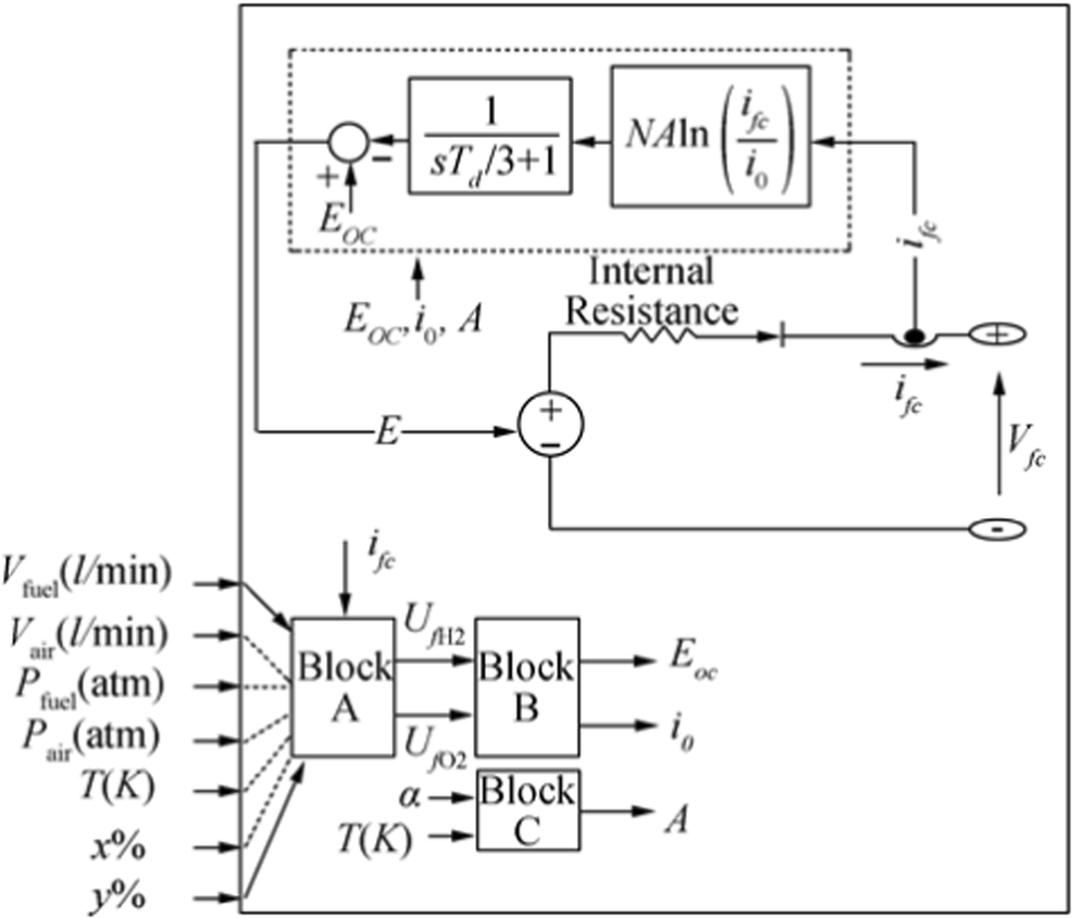Figure  2  Fuel cell equivalent circuit diagram (Tremblay et al. 2009)

Download: Full-Size Img

The controlled voltage source E is described by (Tremblay et al. 2009):

Thus,

where E_oc is the open-circuit voltage (V); N the number of cells; A the Tafel slope (V); I_{_0} the exchange current (A); T_{_d} the response time (at 95% of the final value) (s); R_internal the internal resistance (Ω); I_{_fc} the fuel cell current (A); and V_{_fc} the fuel cell voltage (V).

The open-circuit voltage E_{_oc}, the exchange current i_{_0} and the Tafel slope A are calculated using the set of equations given below:

where F is 96485 A/s/mol; z the number of moving electrons (z = 2); E_{_n} the Nernst voltage (V); a the charge transfer coefficient; P_{_H2} the partial pressure of hydrogen inside the stack (atm); P_{_O2} the partial pressure of oxygen inside the stack (atm); k the Boltzmann's constant (1.38 × 10⁻²³ J/K); h the Planck's constant (6.626 × 10⁻³⁴ J/s); ΔG the activation energy barrier (J); T the temperature of operation (K); and K_c the voltage constant at nominal condition of operation.

Furthermore, the rates of conversion needed from the model are given by (Tremblay et al. 2009):

These quantities express the utilization of hydrogen and oxygen respectively which is key for calculating partial pressures inside the cell:

The Nernst voltage can be now calculated (Genduso and Miceli 2011):

where P_{_fuel} is the absolute supply pressure of fuel (atm); P_{_air} the absolute supply pressure of air (atm); V_{_fuel} the fuel flow rate (l/min); V_{_air} the air flow rate (l/min); x the percentage of hydrogen in the fuel (%); y the percentage of oxygen in the oxidant (%); P_{_H2} the partial pressure of water hydrogen (atm); P_{_O2} the partial pressure of oxygen (atm); P_{_H2O} the partial pressure of water vapour (atm); and W the percentage of water vapour in the oxidant (%).

2.1   Hydrogen, Oxygen and Air Consumption

At standard temperature and pressure (STP), 273.15 K and 100 kPa, the Avogadro number N_a, 6.0221023, expresses the number of molecules in the container in 1 mol of substance. For each kilomolar of hydrogen that reacts, a total of two electrons are released and the produced electric charge is equal to 192.970 C (2Nae). 1 kmol of hydrogen gas occupies 22.41 l which corresponds to an electric current of 192.970 A. Thus, to produce 1 A, the minimum required volumetric flow rate of hydrogen at STP is equal to:

The fuel cell's chemical reaction dictates a 2:1 ratio for hydrogen/oxygen volumetric and water proportion. This ratio is equivalent to 4.76 for the mass flow rate. Given that air in standard conditions contains 21% oxygen and 79% nitrogen by volume, the air volumetric flow rate ratio to react with the same amount of hydrogen rises to 34.

We have seen that the rate of hydrogen, oxygen and air usage is a function of the cell current and the number of cells:

Table 2 summarizes all the equations needed to model the fuel cell system.

3   DC Boost Converter

DC converters have been widely used since the advent of semiconductors and power electronics. These devices are commonly adopted to accomplish voltage regulation tasks for a multitude of applications: from renewable energy power plants to military, medical and transportation systems (Mohan and Robbins 2003).

A non-regulated DC voltage input is converted into a regulated DC output, regardless of operational conditions. Switching devices, such as power MOSFETs are used in this end. For a given input voltage, the average output voltage is regulated by controlling the duty cycle of the semiconductor (Mohan and Robbins 2003).

Boost converters are extensively used to step-up an unregulated input voltage to a stable output. A typical circuit diagram of a DC boost converter includes a power MOSFET, an inductance L, a capacitance C and a diode as shown in Figure 3. When power MOSFET is turned on (0 < t < t_{_on}), the diode does not conduct; thus, the output port is disconnected from the input port and the inductor accumulates the energy provided by the voltage input. On the other hand, when the power MOSFET is turned off (t_{_on} < t < T_{_s}), the output port can absorb power from the inductance and the input source. A DC boost converter has two operating modes: continuous conduction mode (CCM) and discontinuous conduction mode (DCM). We assume a CCM for the converter investigated in this work (Mohan and Robbins 2003).

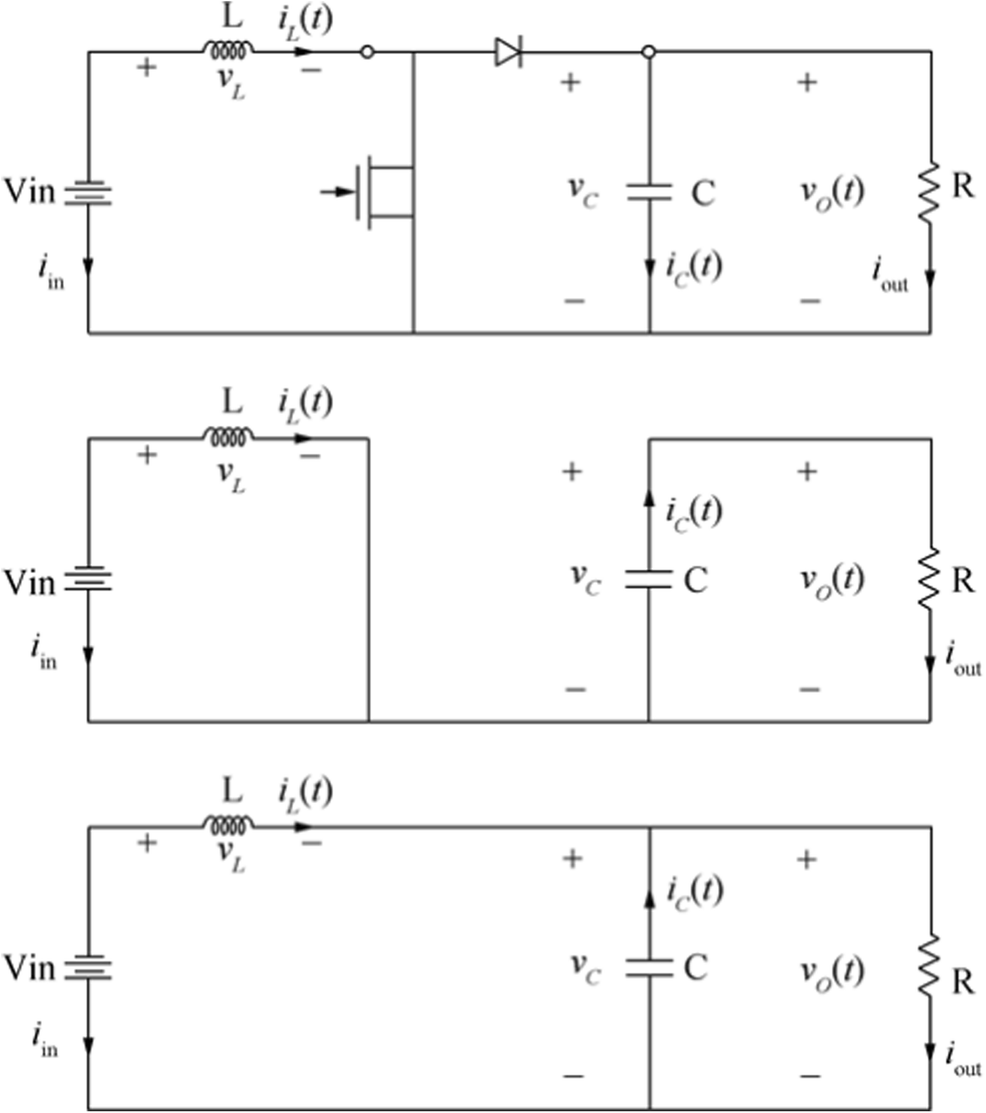Figure  3  DC boost converter topology (top). Steady-state equivalents using ideal elements for 0 < t < t_{_on} (middle) and t_{_on} < t < T_{_s} (bottom) (Mohan and Robbins 2003)

Download: Full-Size Img

3.1   Continuous Conduction Mode

While in this mode, the inductor current is always on, i.e. i_{_L(t)} > 0. The average energy stored over a switching cycle of period T_{_s} in the inductor L is therefore zero at steady state. In result, the average change in inductor current is zero; thus (Figure 4), the following is obtained (Mohan and Robbins 2003):

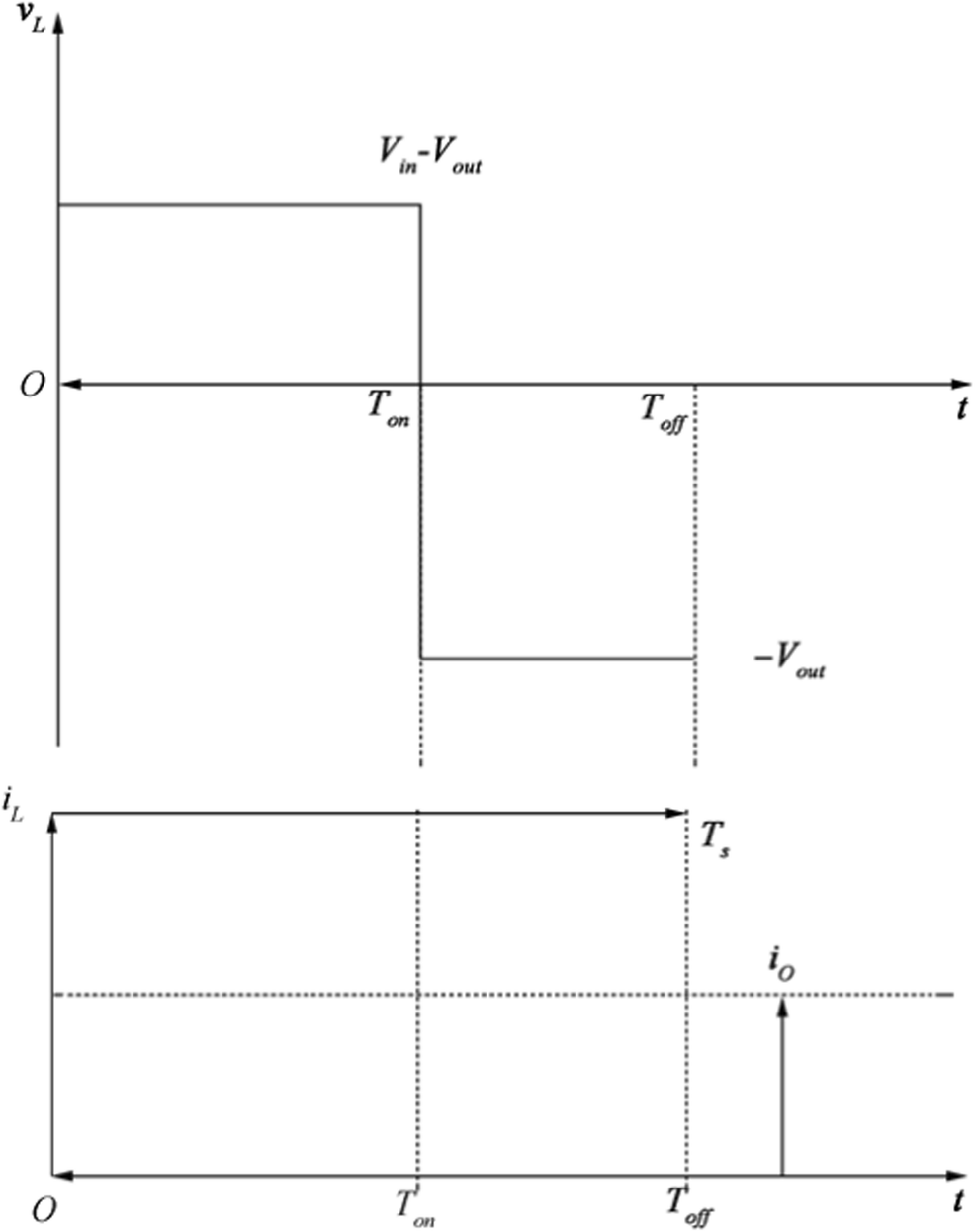Figure  4  CCM inductor voltage (top). CCM inductor current (bottom) (Mohan and Robbins 2003)

Download: Full-Size Img

where i_{_L} is the inductor current; V_{_in} the input voltage; V_{_out} the output voltage; V_{_c} the capacitor voltage; T_{_s} the switching period; T_{_on} the transistor ON time; T_{_off} the transistor off time; and D the duty cycle.

Assuming a lossless device:

where P_{_in} is the input power; P_{_out} the output power; I_{_in} the input current; and I_{_out} the output current.

4   Artificial Neural Network

An artificial neural network (ANN) is an adaptive, often nonlinear system that learns to perform a function (an input-output map) from data. To calibrate (or train) a net, an input and the corresponding desired or target response set at the output need to be presented to the untrained ANN (Galushkin 2007). Broadly speaking, there are three main types of ANN based on the learning approach:

• supervised learning type

• reinforcement learning type

• self-organizing (unsupervised learning) type

Figure 5 shows a fundamental representation of an ANN structured in three layers:

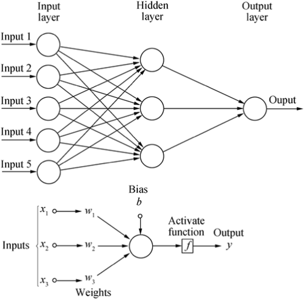Figure  5  ANN architecture diagram

Download: Full-Size Img

• the input layer, where there is no real processing done, is essentially a "fan-out" layer where the input vector is distributed to the hidden layer.

• the hidden layer, being the computational core of the ANN

• the output layer, which combines all the "votes" of the hidden layer

The general mathematical expression that describes an ANN is (Galushkin 2007):

where x is the input vector; y, the output vector; f, activation function; u, weight matrix between hidden and output layer; w, weight matrix between input and hidden layer; and b, biases.

First, the input x is multiplied by the weight w_{_n}. Second, the weighted input xw_n is added to the scalar bias b to form the net input n. The bias is similar to a weight, except that it has a constant input of 1. Finally, the net input is passed through the transfer function f, which produces the output y. The names given to these three processes are the weight function, the net input function and the transfer function. The quantities w_n and b are both adjustable. The central idea here is that such parameters can be adjusted so that the network exhibits the desired behaviour. Thus, one can train the network to accomplish a particular task by adjusting the weight or bias parameters.

By expanding Eq. (22) to a more detailed, elemental form (Galushkin 2007):

where p is the number of input nodes; M, the number of hidden nodes; and K, the number of output nodes.

The activation function f is commonly chosen to be one of the following:

• the logistic sigmoid function (Figure 6), commonly abbreviated as logsig

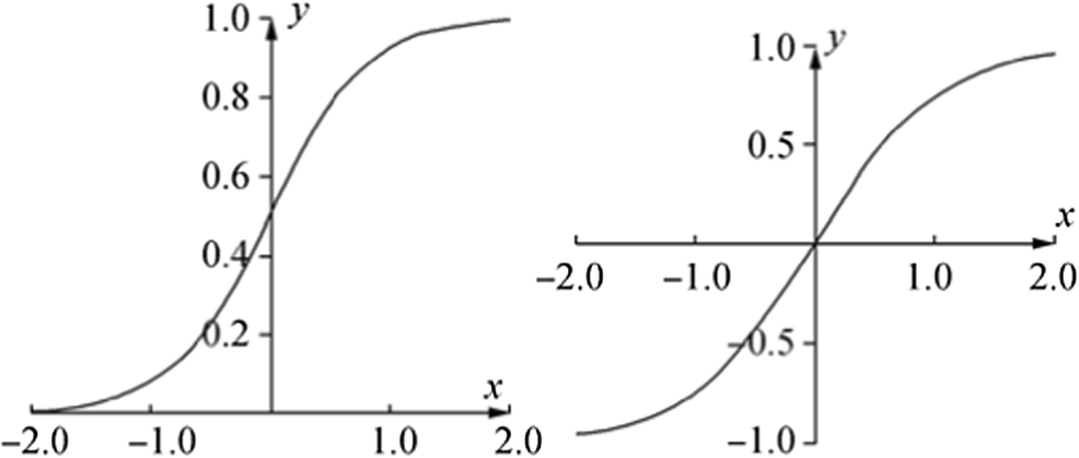Figure  6  Logistic sigmoid function (left). Hyperbolic tangent function (right)

Download: Full-Size Img

• the hyperbolic tangent function (Figure 6), commonly abbreviated as tansig

4.1   Change in Error Due to Output Layer Weights (Self-Learning System) (Galushkin, 2007)

According to the least mean square (LMS) algorithm, the output error is given by:

The partial derivative with respect to the output layer weights u_kj is given by.

By substituting (24) and (27) into (28):

where

The last equation represents the back-propagating error related to the hidden layer output.

where η and μ are positive-valued scalar gains (also called learning constants), typically relatively small values (η, μ < 1) are used. The learning constants adjust the learning rate and govern convergence properties of the backpropagation training process.

4.2   Weight Adjustments (Self-Learning System) (Galushkin, 2007)

Minimizing the output error requires calibration of all weights in the opposite direction of the error gradient each time a training input-output vector is presented to the network undergoing training.

Output and hidden layer weights are adjusted according to the following rules:

where η and μ are positive-valued scalar gains or learning constants, relatively small (η, μ < 1).

5   Steady-State Operation

Simulation studies are crucial in power electronics to essentially predict the behaviour of the device before any hardware implementation. General requirements, design specifications together with control strategies, can be iteratively tested using computer simulations.

5.1   Fuel Cell Generic Model

An outline of the fuel cell model employed was given in previous sections, primarily based on (Tremblay 2009). The aforementioned implementation however uses some input parameters, commonly found in most manufacturers' datasheet.

These parameters are summarized below and remain constant over each simulation time step:

• Current and voltage at the operating point: I_{_nom}, V_{_nom}

• Current and voltage at the maximum operating point: I_{_max}, V_{_min}

• Open-circuit voltage: E_{_oc}

• Voltage at 1 A: V_{_1}

• Nominal operating temperature: T in Kelvin

• Number of cells in series: N

• Nominal composition of fuel and oxidant: x_{_nom}, y_{_nom} (%)

• Nominal oxidant pressure at stack input: P_{_air} (atm)

• Charge coefficient: a

• Nominal stack efficiency: n_{_eff} (%)

5.1.1   Configuration of Fuel Cell Parameters

For the scope of this work, a commercial off-the-shelf (COTS) 6-kW PEMFC is considered (Tremblay 2009).

The parameters given as inputs to the model are summarized in Table 3.

5.2   Fuel Cell Model Validation

The polarization curves of both simulated and experimental data (as per datasheet), for the commercial 6-kW PEMFC considered are overimposed in Figure 7. Experimental data are represented with a solid line while the dashed line shows the simulated results. The ohmic region (50 to 225 A), a linear gradual drop in voltage attributed to the ohmic resistance in the cell and the depletion of the reactive gas at the catalyst surface, exhibits similar behaviour in both cases; hence, the two curves coincide. The activation region (0 to 50 A) however, a sharp voltage drop attributed to the type of catalyst and the catalyst surface, does not exactly match the experimental curve due to the nonlinearity of the activation voltage. Additionally, the polarization curve of the PEMFC for a specific volumetric fuel flow rate is obtained (the air flow is bounded by the stoichiometry of the reaction) and shown in Figure 8.

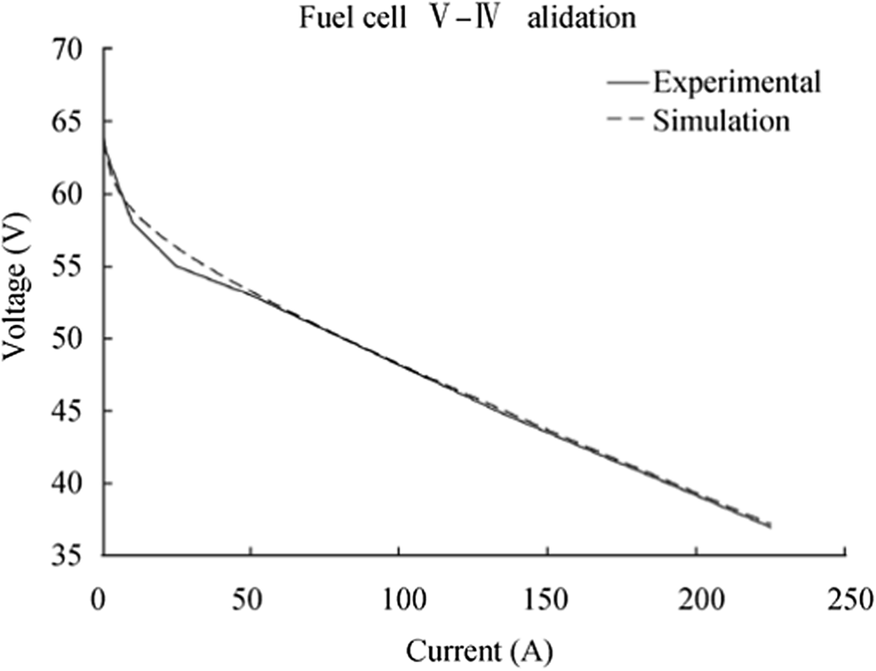Figure  7  Experimental and simulated data for a 6 kW COT PEMFC (1.5-atm fuel pressure, 50-lpm fuel flow, 300-lpm air flow)

Download: Full-Size Img

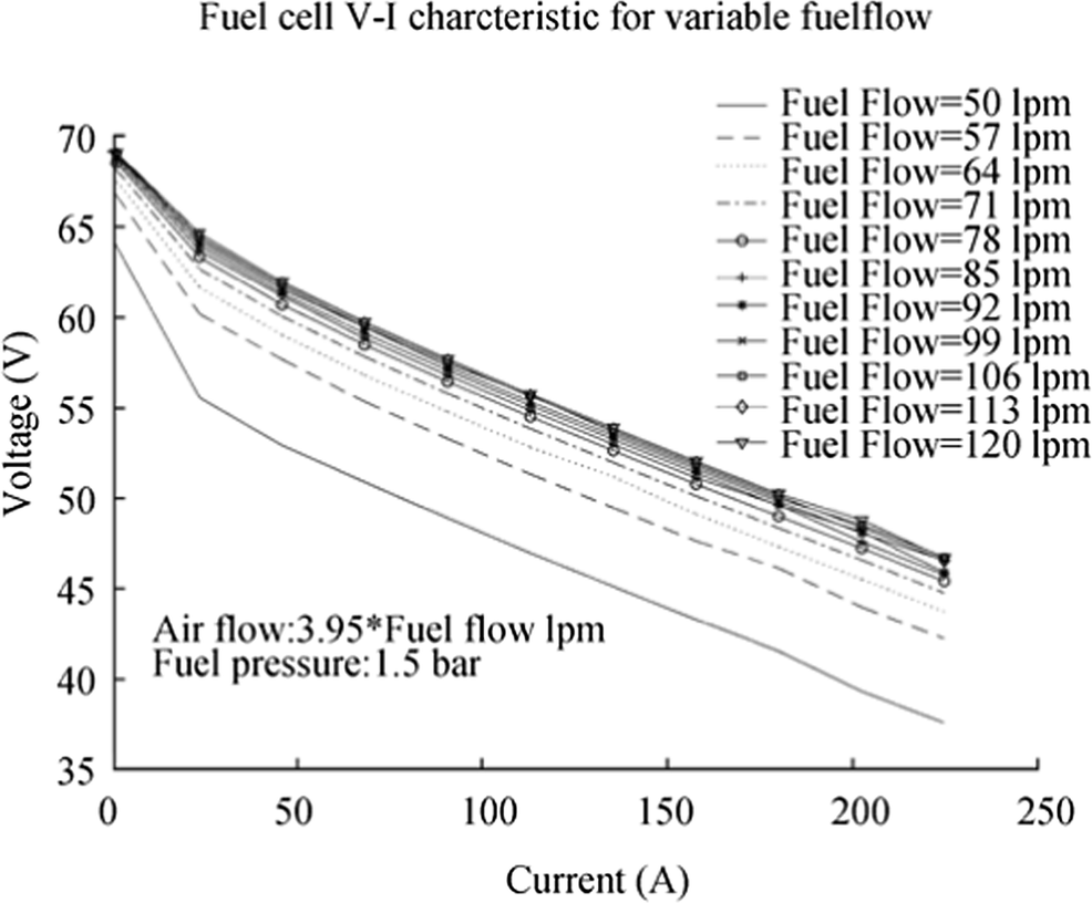Figure  8  Simulation results of fuel cell I–V characteristic for variable fuel flow

Download: Full-Size Img

5.3   DC/DC Boost Converter Switching Model

Converter efficiency and cost are the main requirements driving its topology design. Before modelling the system, several design assumptions and calculations need to be explained, especially pertaining to the L and C elements. The following design is neither bound to nor optimized for specific I–V curves; thus, it is expected to operate with a variety of PEM fuel cells.

5.3.1   Inductor Selection

The critical inductance is defined as the inductance at the boundary edge between continuous and discontinuous modes. The input current at the boundary between CCM and DCM is equal to the inductance current and on average:

Using Eq. (17), we can simplify (38) as:

And the output current is calculated as:

By substituting

The minimum inductance required is given by:

5.3.2   Capacitance Selection

The ripple voltage at the output is given by the equation:

where ΔQ is the change in the capacitor charge.

Dividing (41) by V_{_out}, we obtain:

To limit the peak-to-peak output voltage ripple to some desired value, the minimum capacitance required is given by:

where V_{_cpp} is the peak-to-peak output voltage ripple.

5.3.3   Selection of the Semiconductor Device (MOSFET (Mohan and Robbins 2003))

The power MOSFET must handle the worst case where the current input to the DC converter is maximum, thus:

where I_{_MOSFETmax} is the MOSFET maximum current; I_{_fcmax} the fuel cell maximum current; and ΔI_{_fcmax} the fuel cell maximum overcurrent.

Other important considerations in selecting the diode besides its ability to block the required off-state voltage stress and have sufficient peak and average current handling capability are fast-switching characteristics, low reverse recovery and low forward voltage drop.

5.3.4   Diode Selection

Similar to the semiconductor, the worst-case scenario regarding peak current occurs for low voltage input and high output load. The boost diode reverse voltage rating is limited to the output voltage.

Calculations pertaining to the important design operational parameters are tabulated below for the system in the test case considered:

Table 3 summarizes the main operational parameters for the considered converter.

5.3.5   Model Implementation

Modelling of power electronic converters presents many challenges: the nonlinearity of solid-state switches, too long simulation times due to the presence of time constants which differ by several orders of magnitude and inaccuracies in the models of semiconductor devices are some among them. The power switch, for the scope of this work, is treated as an ideal two states (on-off) component. In order to meet the requirements introduced by the high switching frequency, very small time steps are needed, making the model computationally demanding. For this particular reason, the model is run for only a short period of time. The aim of this particular simulation is to validate the model against the converter behaviour and generate sets of data useful to for ANN training.

The voltage output is a function of input voltage, duty cycle and external load:

Figure 9 shows the open-loop DC-DC boost converter output voltage and inductor current for a constant duty ratio equal to 0.55, an input voltage of 45 V, under different load cases: 28 Ω (0–2 s), 20 Ω (2–4 s), 10 Ω (4–6 s), 5 Ω (6–8 s), 2.5 Ω (8–10 s) and 2 Ω (10–12 s).

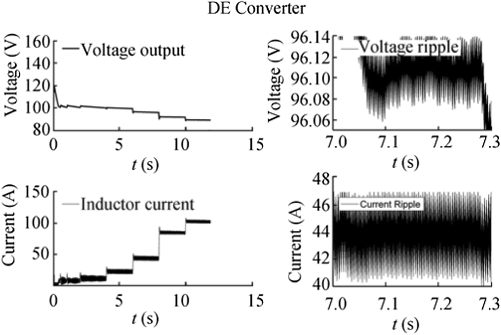Figure  9  Output of open-loop DC boost converter: voltage output (top left), voltage ripple (top right), inductor current (bottom left), inductor current ripple (bottom right)

Download: Full-Size Img

From the results depicted above, it is clear how the output voltage does not reach the expected value of 100 V, but exhibits a ± 10% variation. The output signal however shows a good degree of stability. During start-up, there is a high overshoot in the output voltage and inductor current. This current increases as we increase the load. The unsatisfactory voltage level response along with the relatively long settling time clearly demonstrates the need for a controller.

5.4   ANN configuration for DC/DC boost converter control

The ANN designed to approximate the DC/DC boost converter and control its duty cycle is configured essentially based on the architecture shown in Figure 5. The workflow for any of these networks has the following steps:

• Collect data

• Create the network

• Configure the network

• Initialize the weights and biases

• Train the network

• Validate the network

• Use the network

Essentially, the two ANNs address different problems by executing different tasks:

• Control, by generating a control input signal such that the dynamic system output follows a desired trajectory

• Function approximation, where a set of training data is generated from a complex function and the ANN estimates the output of the function

The controlling ANN is a feed-forward network organized in layers: an input layer, a hidden layer and an output layer. The size of each layer is defined by the number of neurons, e.g. 3-5-1 is an ANN composed of 3 layers. The input layer has 3 neurons and the hidden layer 5 neurons while the output layer 1 neuron. The input neurons correspond to the number of inputs according to the system design, while the hidden layer size is a trade-off between simplicity and accuracy. The output neuron generated the control signal.

In this work, the hidden layer size is set to a range from 7 to 14 neurons. The final neuron number is 9 defined as a function of output error and simplicity. Training is accomplished using the neural network toolbox provided by Matlab MathWorks (The MathWorks, Inc.). The weight and bias values are updated according to Levenberg-Marquardt optimization. It minimizes a combination of squared errors and weights and then determines the correct combination so as to produce a network that generalizes well. The process is called Bayesian regularization.

5.4.1   Generation of ANN Data

The training data set for the ANN corresponds to the input voltage, the output voltage the external load and the duty cycle. In order to generate this data, a total of 512 runs were conducted for varying input voltages, duty cycles and external load according to Table 4.

5.4.2   ANN Data Parameterization and Separation for Training and Validation

The data presented to the ANN network for training and validation are a N∈R3 × n matrix with n = 512 and a M∈R1 × m with m = 512. Each column represents a data set, for a total of 512 data sets fed to the ANN for training.

An example of the final data arrangement is as follows:

5.4.3   ANN Implementation and Training

The ANN was implemented and trained using the Matlab Neural Network Toolbox Mathworks (The MathWorks, Inc.). A number of different ANNs were tested in order to conclude the best combination of simplicity and network performance, with the hidden layer ranging from a minimum of 7 neurons to a maximum of 14 neurons. The selected training algorithm is the Levenberg-Marquardt; 70% of the data is used for training, 15% for validation, and the remaining 15% for testing.

Figures 10, 11, 12, 13, 14, 15, 16 and 17 show the ANN performance for different network sizes (7–14) with regard to the converter output. The dashed line represents the perfect result: outputs = targets. The solid line represents the best-fit linear regression line between trained net outputs and targets. The R value is a correlation indicator between outputs and targets. If R = 1, there is an exact linear relationship between outputs and targets. If R = 0, then there is no linear relationship between outputs and targets (Choi et al. 2004). All cases show a good approximation of the converter output by the ANN. Thus, the final network is of type 3-9-1, being a combination of performance and simplicity.

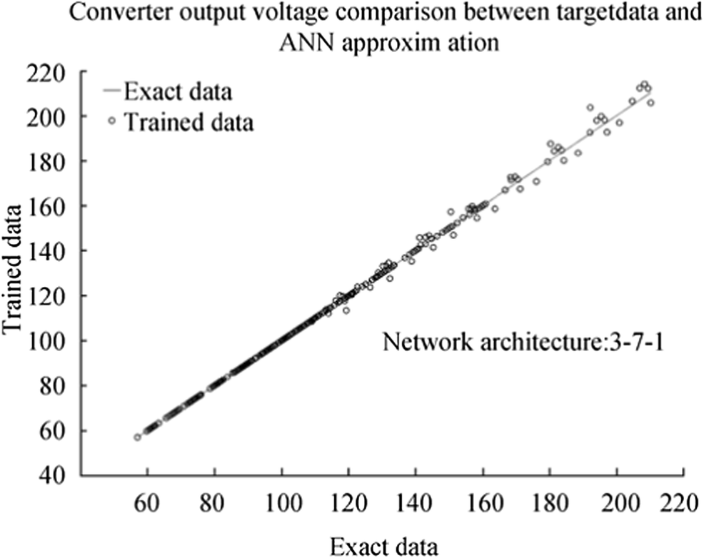Figure  10  DC/DC converter ANN analogue performance for hidden layer size 7

Download: Full-Size Img

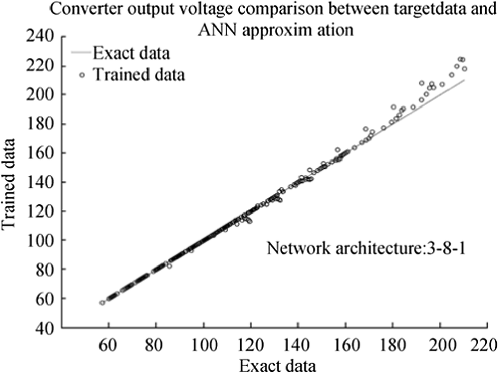Figure  11  DC/DC converter ANN analogue performance for hidden layer size 8

Download: Full-Size Img

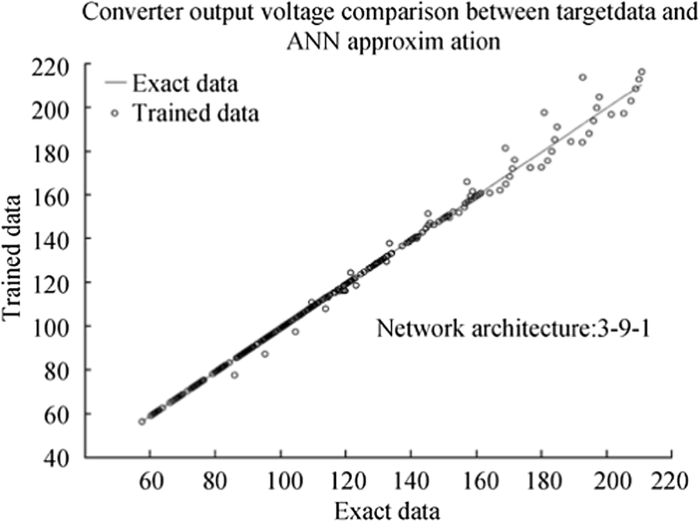Figure  12  DC/DC converter ANN analogue performance for hidden layer size 9

Download: Full-Size Img

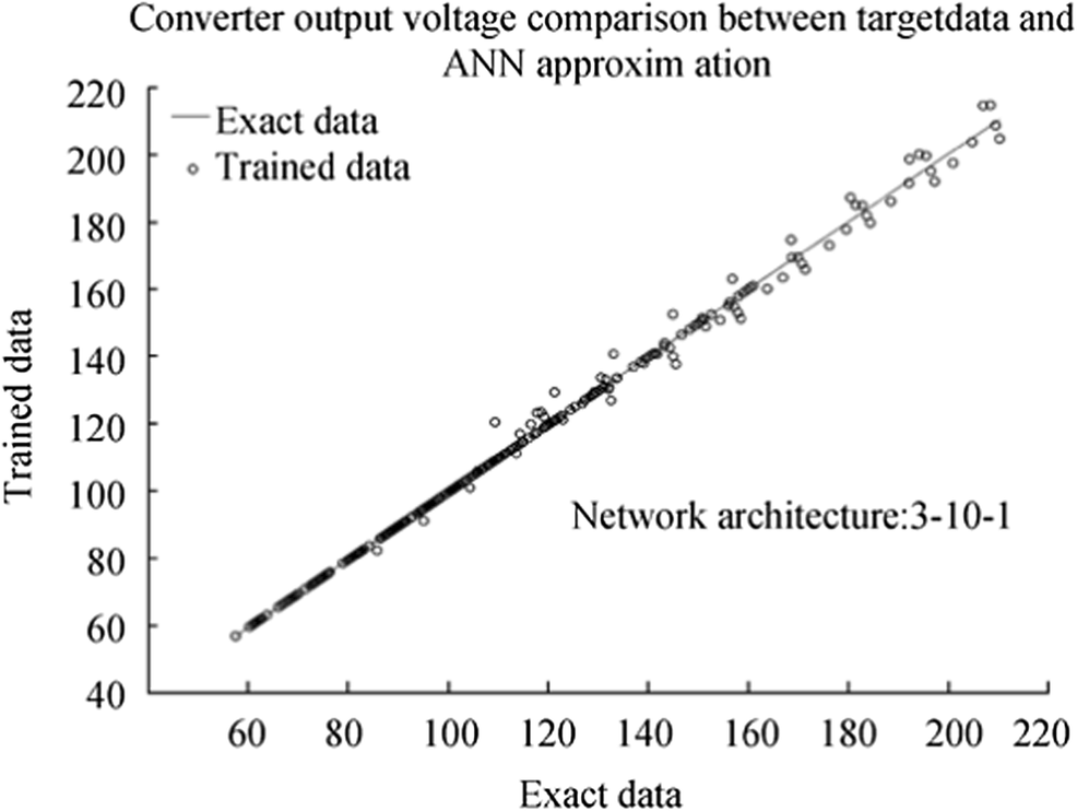Figure  13  DC/DC converter ANN analogue performance for hidden layer size 10

Download: Full-Size Img

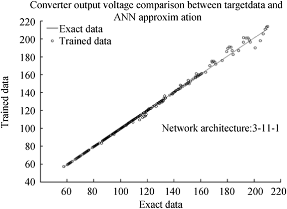Figure  14  DC/DC converter ANN analogue performance for hidden layer size 11

Download: Full-Size Img

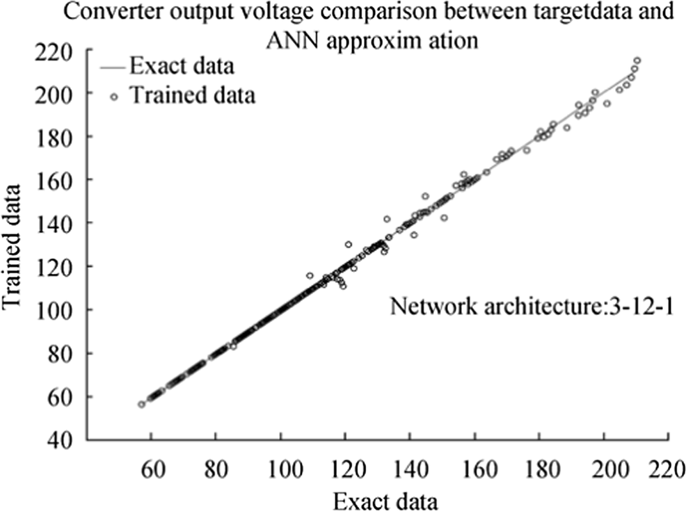Figure  15  DC/DC converter ANN analogue performance for hidden layer size 12

Download: Full-Size Img

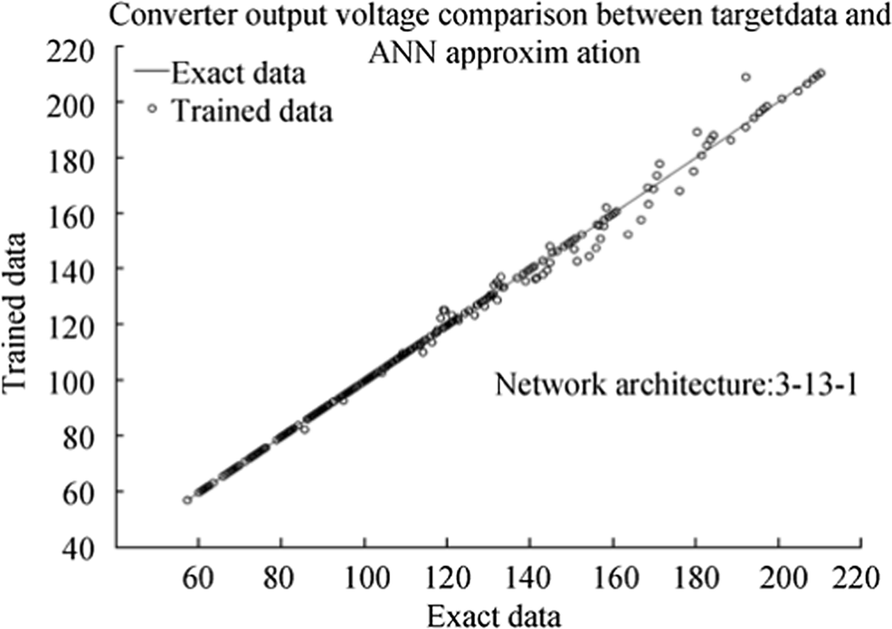Figure  16  DC/DC converter ANN analogue performance for hidden layer size 13

Download: Full-Size Img

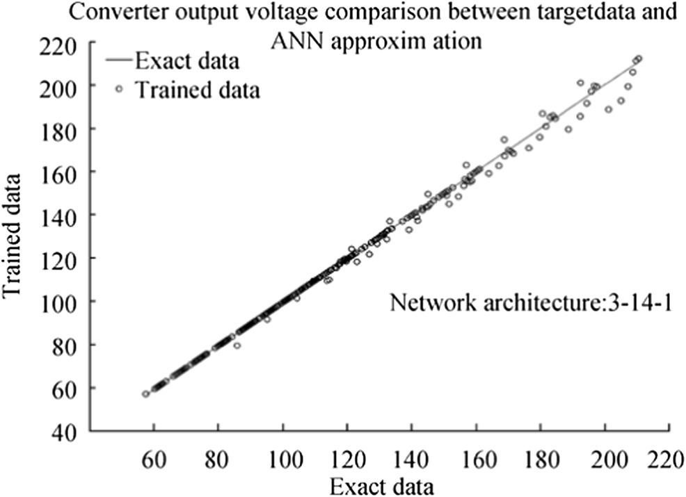Figure  17  DC/DC converter ANN analogue performance for hidden layer size 14

Download: Full-Size Img

Figures 18, 19, 20, 21, 22, 23, 24 and 25 show the ANN performance for different network sizes (7–14) with regard to duty cycle. All cases indicate a good fit, with the scatter manifesting the data points exhibiting a poor fit.

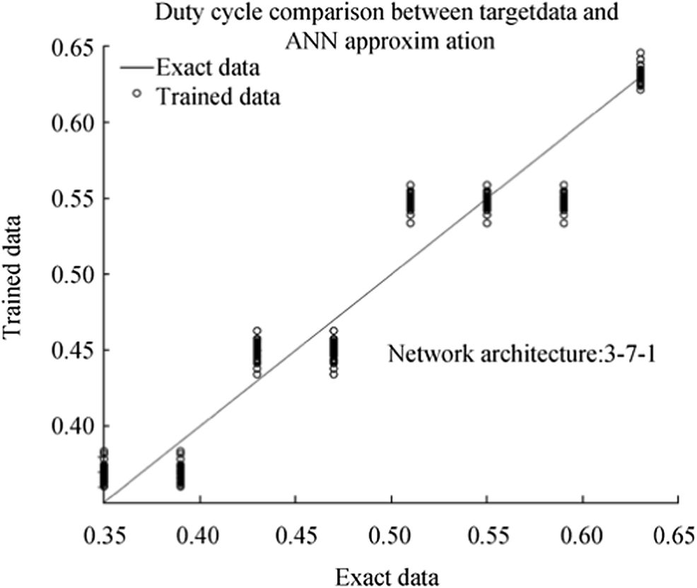Figure  18  ANN converter control performance for layer size 7

Download: Full-Size Img

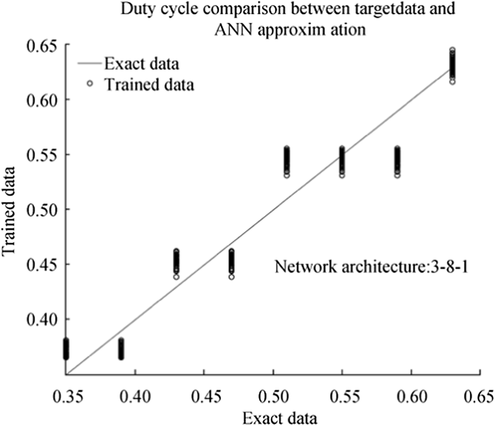Figure  19  ANN converter control performance for layer size 8

Download: Full-Size Img

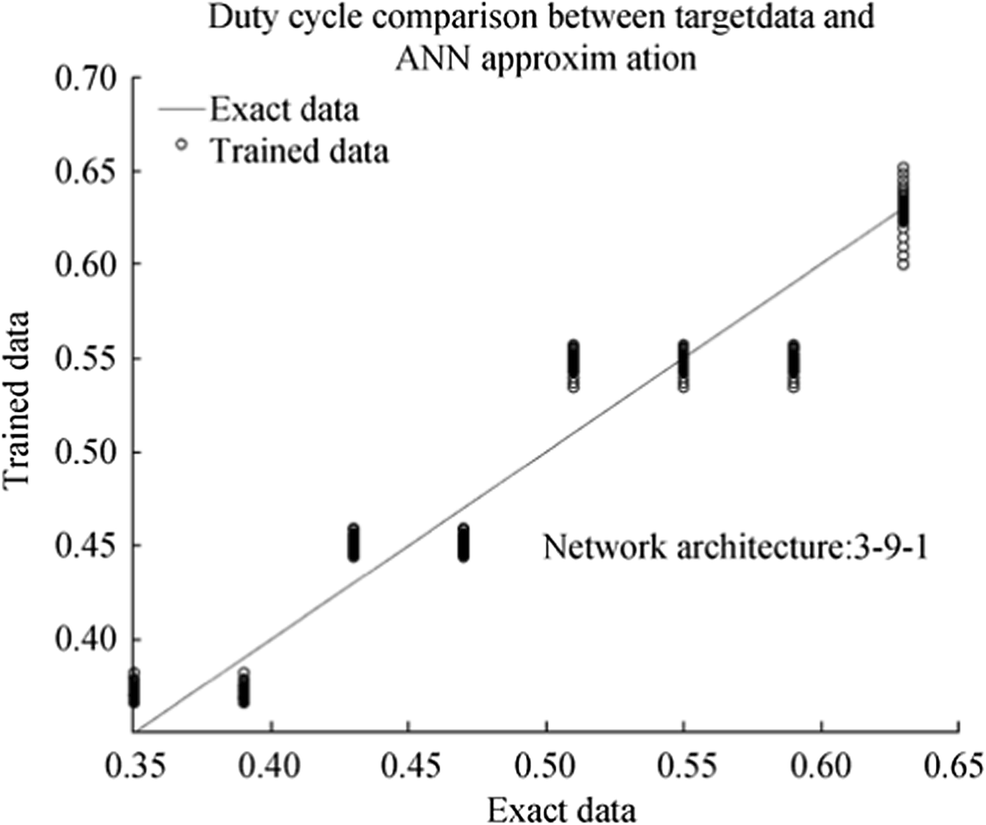Figure  20  ANN converter control performance for layer size 9

Download: Full-Size Img

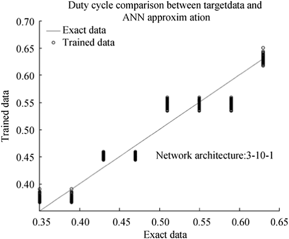Figure  21  ANN converter control performance for layer size 10

Download: Full-Size Img

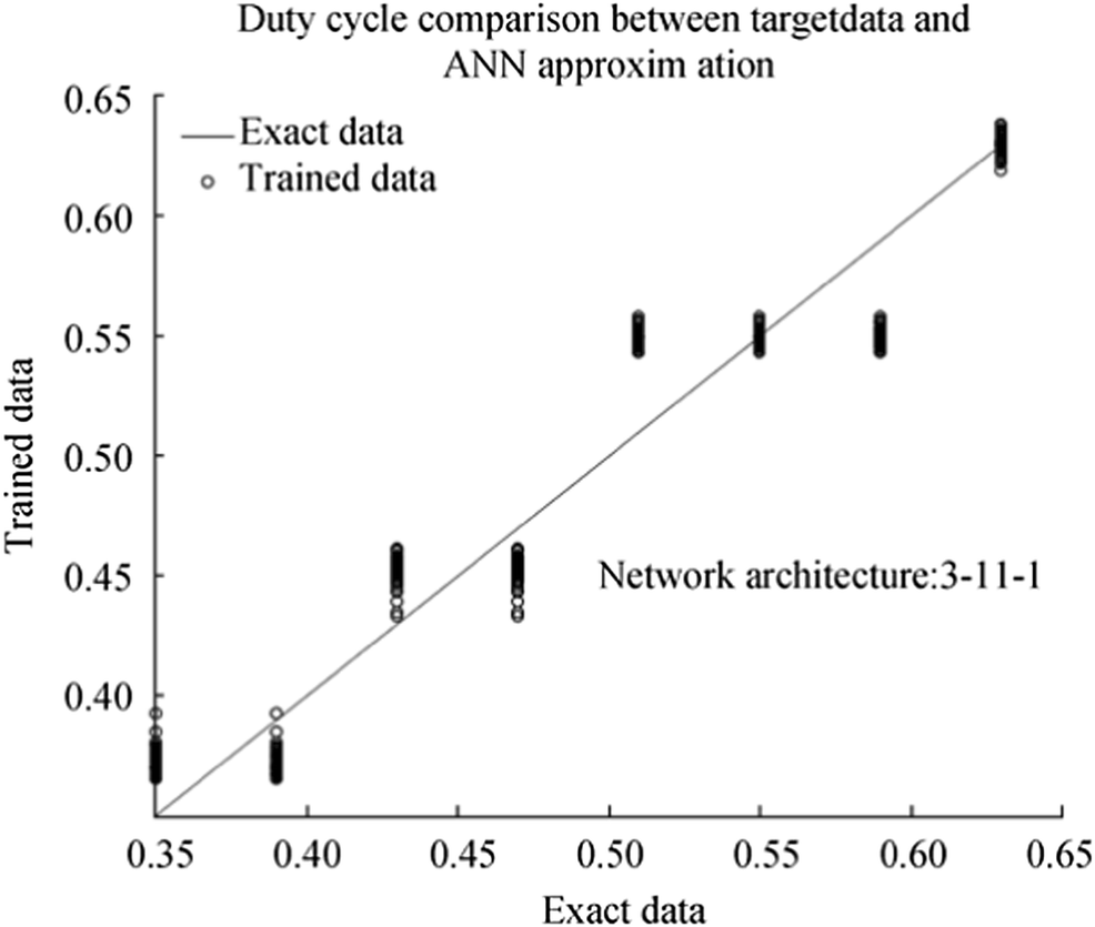Figure  22  ANN converter control performance for layer size 11

Download: Full-Size Img

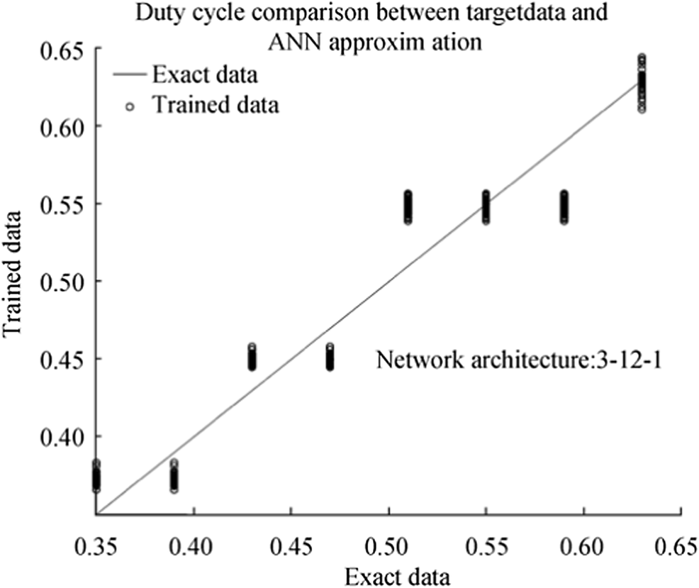Figure  23  ANN converter control performance for layer size 12

Download: Full-Size Img

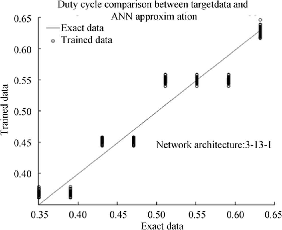Figure  24  ANN converter control performance for layer size 13

Download: Full-Size Img

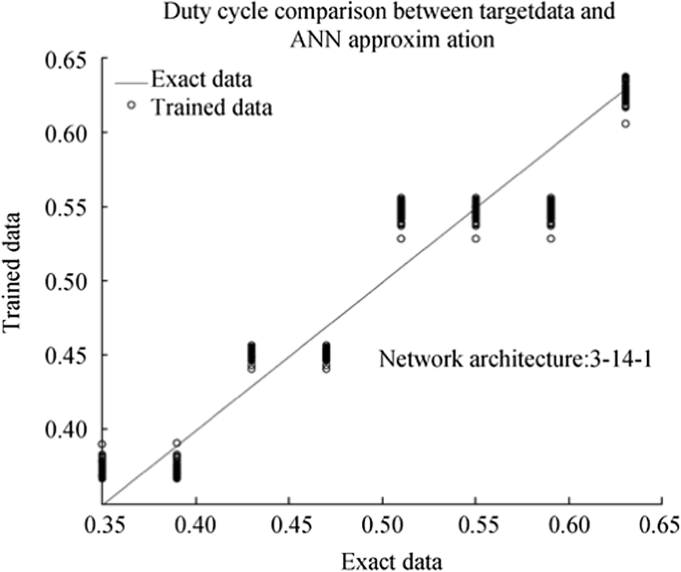Figure  25  ANN converter control performance for layer size 14

Download: Full-Size Img

6   Dynamic System Operation

In this section, the full system behaviour under dynamic conditions is studied. The standalone subsystems are connected together according to Figure 1, where the output fuel cell voltage is fed to a DC converter, in order to sustain a stable bus voltage for a resistive load (consumer).

Initially, an open-loop simulation is performed where no feedback control is present.

Next, the trained ANN is presented to the switching model of the DC-DC converter. The ANN is controlling the duty cycle, reacting to load changes and any voltage variation at the converter input.

Finally, the switching model of the DC-DC converter has been substituted by an ANN cycle-to-cycle equivalent. Control is applied in this case as well.

The final model, however, is based upon several assumptions:

• The gases are assumed ideal.

• The stack is fed with hydrogen and air.

• The stack is equipped with a cooling system which maintains the temperature at the cathode and anode exits stable and equal to the stack temperature.

• The stack is equipped with a water management system to maintain the humidity inside the cell at an appropriate level at any load.

• The cell voltage drops are due to reaction kinetics and charge transport as most fuel cells do not operate in the mass transport region.

• Pressure drops across flow channels are negligible.

• The cell resistance is constant at any condition of operation.

• Storing conditions of fuel and oxidant are not taken into account.

• Semiconductor devices are assumed to act as ideal switches.

The following variables are recorded during all simulation cases:

• Hydrogen flow rate

• Fuel cell voltage

• Fuel cell current

• Fuel cell power output

• Load power demand

• Load voltage/converter output voltage

• Load current/converter output current

• Fuel cell efficiency

• Converter inductor current and ripple

• Converter output voltage and ripple

The resistive load changes every couple of seconds. Assuming a DC bus of 100 V the demand is equal to:

• 358 W for 28 Ω

• 500 W for 20 Ω

• 1000 W for 10 Ω

• 2000 W for 5 Ω

• 4000 W for 2.5 Ω

• 5000 W for 2 Ω

6.1   Open-Loop Simulation

In this case, no control is applied to the system. The results are shown in Figures 26, 27 and 28. Figure 26 graphically summarizes the relation between the fuel cell hydrogen flow rate and current, for different load demands, as a function of time. The fuel cell current increases linearly with the load power demand and the fuel cell output voltage according to the equation:

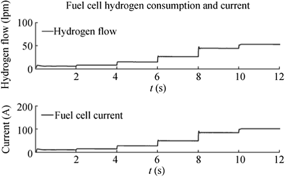Figure  26  Fuel cell hydrogen flow (top) and current for different load demands (bottom)

Download: Full-Size Img

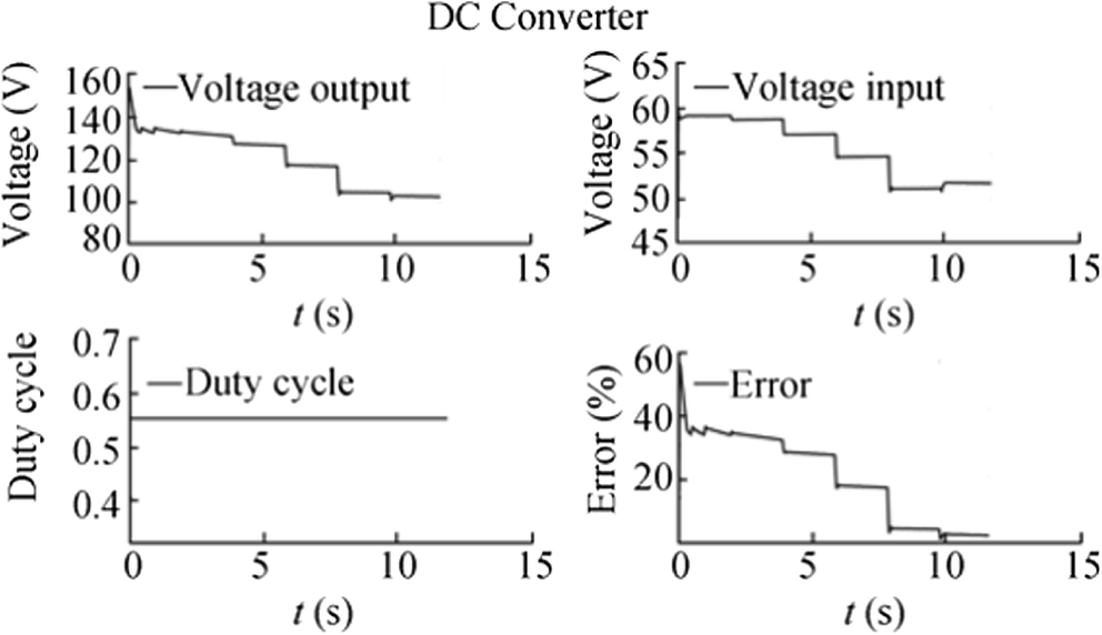Figure  27  DC/DC converter response: voltage output (top left), voltage input (top right), duty cycle (bottom left) and error between output and target voltage (bottom right)

Download: Full-Size Img

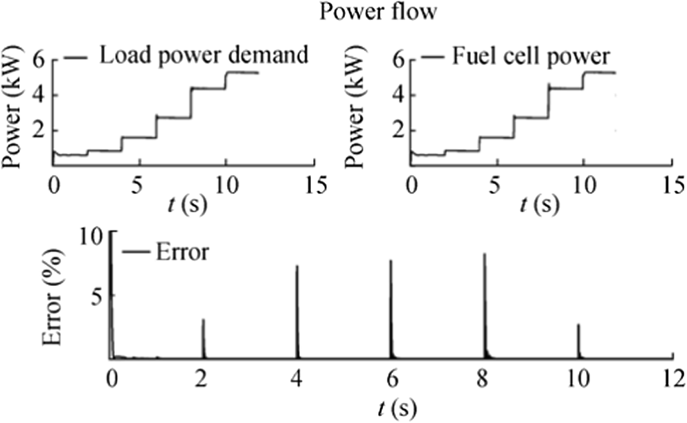Figure  28  Load power demand (top left), fuel cell power output (top right) and power deficit between demand and generation (bottom)

Download: Full-Size Img

where P_{_load} is the load power demand; P_{_fc} the fuel cell power output; V_{_load} the load voltage; I_{_load} the load current; V_{_fc} the fuel cell voltage output; and I_{_fc} the fuel cell current output.

Hydrogen flow responds to this variation following Eq. (12) reaching a maximum value of roughly 50 lpm. The fuel cell response can be optimized by employing control techniques on the hydrogen flow rate based on the desired current.

Figure 27 shows the dynamic response of the DC converter to input voltage and load variations. The duty cycle is kept constant and equal to 0.55 to allow open-loop operation. It is clear how the output voltage never reaches a constant target value but stays constantly above 100 V. The need for a stable and constant DC bus voltage highlights the need for control to be applied on duty cycle side.

The graphs in Figure 28 show the fuel cell power output and the load power demand. The fuel cell power is tied to the demand. As the load power demand rises, monotonically with the load current and by extension the fuel cell current (Eq. 48) and hydrogen flow (Eq. 12), the fuel cell reaches its nominal equilibrium point. One could argue that optimization on the hydrogen flow by means of control will result in higher cell efficiencies, even for low power demand.

6.2   Neural Network Control of Switching DC-DC Boost Converter

The control strategy is based on the neural controller. A previous analysis has shown that the number of hidden layers does not have a serious impact on the controller behaviour and effectiveness. Thus, as a function of output error and simplicity, a 3-9-1 architecture is chosen. The controller ANN task is to generate a correct value for the converter duty cycle, such that the output is stable and as close as possible to the desired target of 100 V. The results are shown in Figures 29, 30, 31, 32 and 33. Figure 29 shows the hydrogen flowing towards the fuel cell and its current. These figures seem to be slightly under the respective values corresponding to the previous simulated open-loop case (Figure 27). This is expected since no means of control are applied to the hydrogen distribution system. Figure 30 depicts the converter response with respect to the voltage output (top left), voltage input (top right), duty cycle (bottom left) and error between output and target voltage (bottom right). It is clear how the controller ANN reacts to variable loads and voltage inputs in order to keep the bus voltage close to the target value. This effect is expressed by the duty cycle response. The load voltage fluctuates between 96 and 99 V with error ranging between 2% and 4%. The voltage ripple of the output voltage signal is kept under 1% according to the converter design (Figure 31). Last but not the least, the fuel cell is capable of delivering the load with the required power meeting the demand throughout all simulation time. According to Mohan and Robbins (2003), only limited amount of ripple current can be applied on a fuel cell. This value changes from system to system, affecting the reactant utilization and eventually impacting on the device lifetime. Figure 33 compares the inductor current ripple applied during the open-loop simulations and the ANN-controlled converter. The controlled device shows a lower magnitude value.

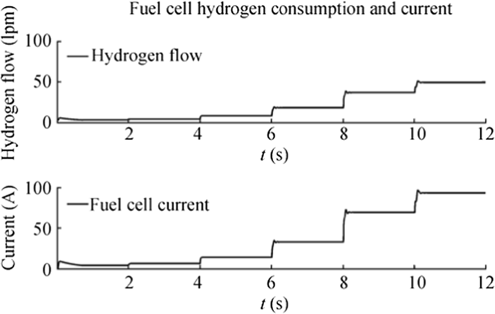Figure  29  Fuel cell hydrogen flow (top) and current for different load demands (bottom)

Download: Full-Size Img

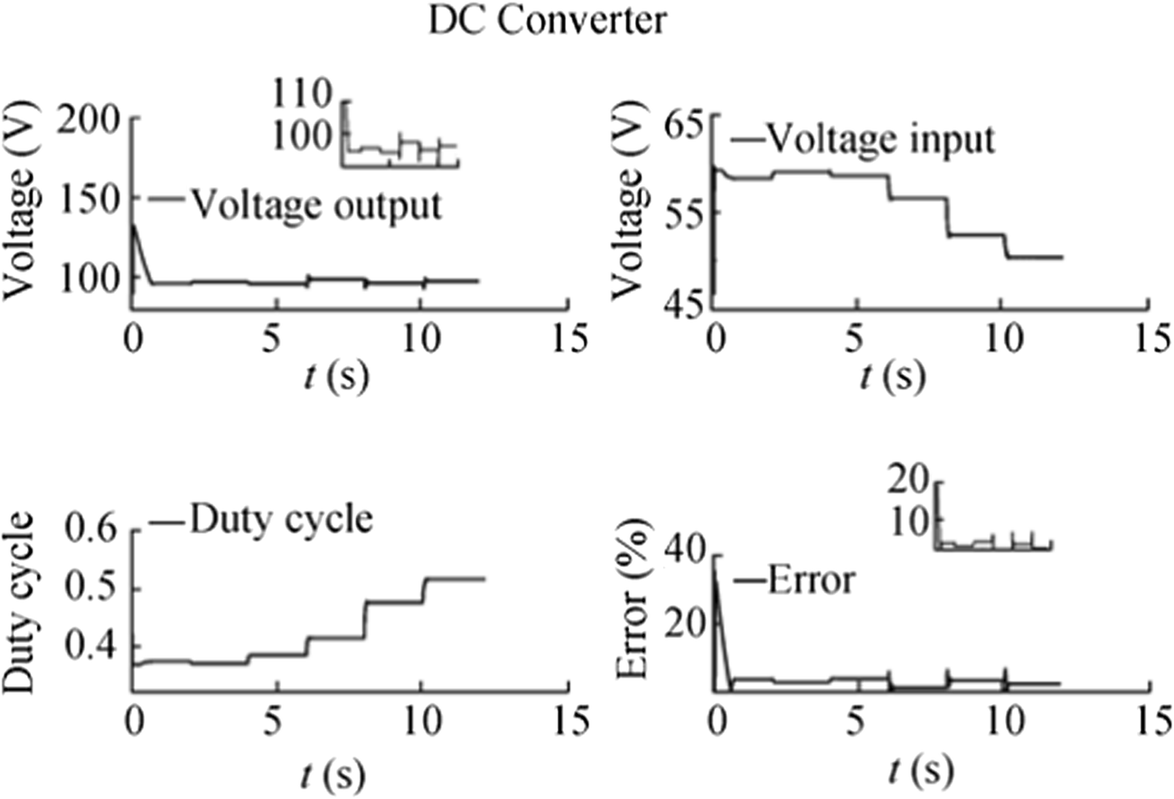Figure  30  DC converter response: voltage output (top left), voltage input (top right), duty cycle (bottom left) and error between output and target voltage (bottom right)

Download: Full-Size Img

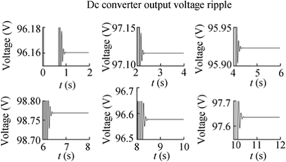Figure  31  DC/DC converter output voltage ripple for various load demand values

Download: Full-Size Img

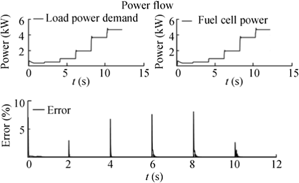Figure  32  Load power demand (top left), fuel cell power output (top right) and power deficit between demand and generation (bottom)

Download: Full-Size Img

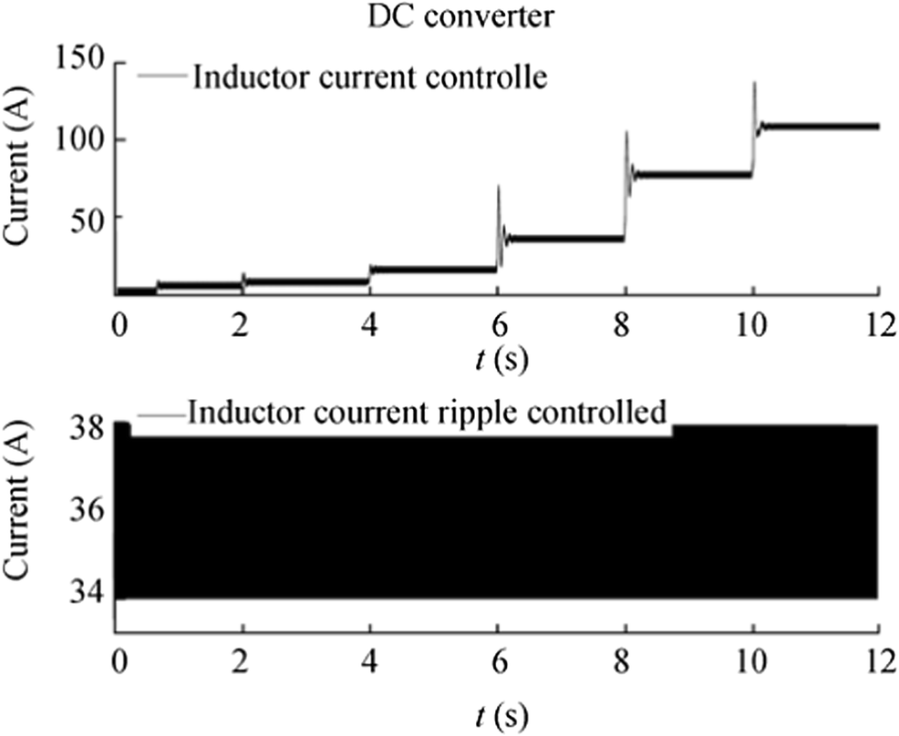Figure  33  DC/DC converter inductor current with closed-loop control (top), inductor current ripple with closed-loop control (bottom left) and inductor current ripple in open-loop configuration (bottom right)

Download: Full-Size Img

6.3   Neural Network Control of ANN DC/DC Boost Converter Cycle-to-Cycle Equivalent

As discussed earlier, the simulation of switching devices is computationally demanding. In this section, the switching model of the DC converter is replaced by its ANN cycle-mean equivalent, the architecture of which is of type 3-13-1. Results are shown in Figures 34, 35 and 36. Transient phenomena cannot be modelled by the ANN equivalent; thus, this model is only useful for system optimization simulation rather than in the transient analysis of converter devices. During the first 6 s of the simulation, the ANN cycle-mean equivalent exhibits a greater disparity from the DC bus target voltage when compared with the switching model. Past this point, the switching model is more precise. This behaviour can be improved by further training of the ANN simulating the DC-DC converter in order to obtain improved results. The inability to model transient phenomena along with a greater voltage excursion, from target values, is the price to pay for faster simulation times.

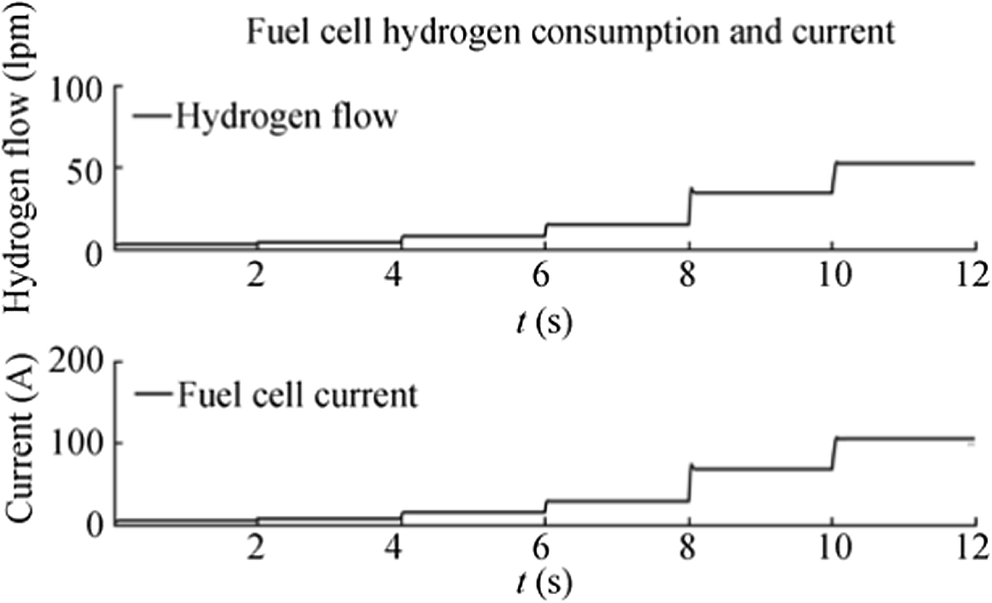Figure  34  Fuel cell hydrogen flow (top) and current for different load demands (bottom)

Download: Full-Size Img

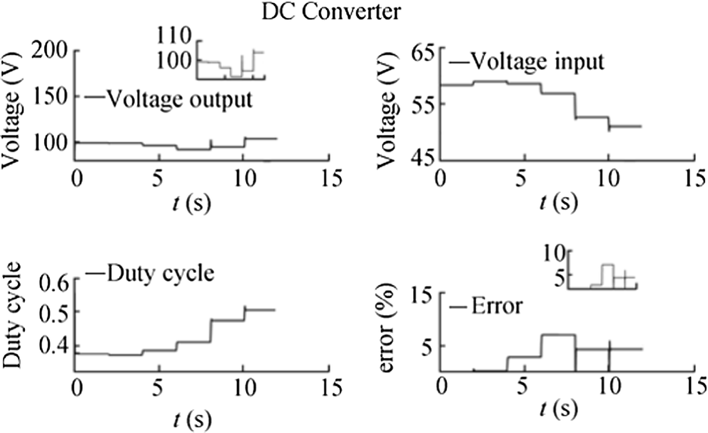Figure  35  DC-DC converter response: voltage output (top left), voltage input (top right), duty cycle (bottom left) and error between output and target voltage (bottom right)

Download: Full-Size Img

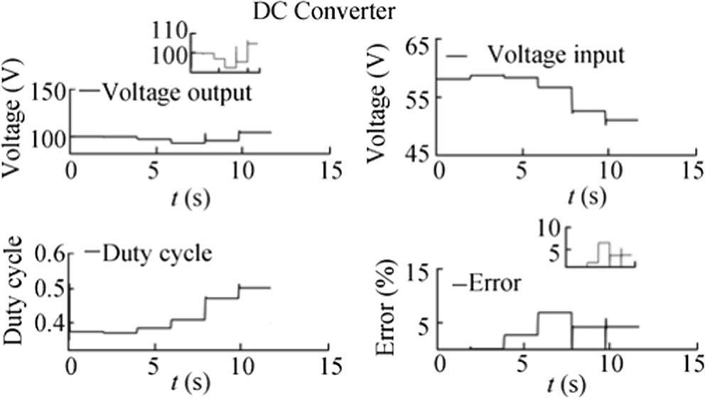Figure  36  Load power demand (top left), fuel cell power output (top right) and power deficit between demand and generation (bottom)

Download: Full-Size Img

7   Conclusions

In this paper, a suite of models for a coupled system including a PEMFC and a DC-DC converter have been developed. Extensive and detailed simulations have been carried out to show how the models are used to characterize the fuel cell's I–V curves and the converter output voltage and control signals, specifically for steady-state operation. Using the models developed and the simulation results, an ANN controller has been configured and tuned for the coupled DC source system consisting of a fuel cell, and a DC-DC converter. In this work, the DC source system was tuned to supply a purely resistive load; however, in the future, more complicated loads will be considered as well. The model is flexible and accurate; specifically, it is able to adapt to different operating conditions, thus suitable for dynamic simulations. The ANN controller compensates satisfactorily for changes in power source input or output.

In literature, oftentimes conventional PI controllers are tuned to regulate DC converter behaviour and supply the desired output voltage level. The results are often compared with neural network control techniques. Both methods are reliable in order to obtain a constant output voltage and system stability. However, the ANN-based controller shows a faster settling time while the terminal voltage overshoot is kept to a minimum. Furthermore, the adjustment and tuning of ANN are more straightforward and enables to build in adaptive and constantly improving regulation schemes. The output voltage error of the system presented in this work is ranging from a minimum of 2% to a maximum of 4%. Performance can be further improved however by allowing the ANN to train with increasing volumes of data sets. Similar systems have been presented in literature; however, the majority addresses the question of optimal control using non-variable voltage inputs to the system. In this respect, it is also of interest to mention the noticeable damping performance of the neural controller which provides for substantial stability margin regardless of how severe the disturbance at the regulator input (fuel cell) or output (load) or joint may be. Additionally, one should notice that the power levels with which this work deals with are considerably higher than the ones commonly encountered in literature.

Last but not the least, a novel approach towards a computationally less demanding architecture suitable for fast simulations was presented. An ANN cycle-mean equivalent model was developed and integrated into the system; such model sufficiently substitutes for the full detailed, yet computationally severely demanding, switching model of the DC-DC converter. The extensive use of appropriately trained ANNs results in a much faster simulation while accuracy of the produced results in terms of output voltage level, and overshoot, current and voltage ripple is essentially not compromised. Future work includes the extension of the method to reactive and nonlinear loads as well as incorporating real-time adaptive features in the controller by employing further big data techniques and AI or computational intelligence, e.g. neuro-fuzzy schemes.