Inverse Optimal Control for Speed-varying Path Following of Marine Vessels with Actuator Dynamics
1 Introduction
Depending on the motion control objectives involved, the following motion control scenarios are often considered for marine vessels: (a) target tracking, (b) path following, (c) path tracking, and (d) path maneuvering. For more details on the motion control scenarios, see Breivik et al. (2008). Path following for marine vessels is an important practical problem. Whether on the surface or under the surface, many offshore activities involve path-following tasks. The control objective of path following is to follow a predefined path, which only involves a spatial constraint. No restrictions are placed on the temporal propagation along the path. Several researches have been carried out in the field of path following, see Fossen et al. (2003), Bibuli et al. (2009), Breivik (2010), and BØrhaug et al. (2008) for instance.
Guidance systems are very important when considering the accuracy of path following. A frequently used method for path following is the line-of-sight (LOS) guidance. The advantage of LOS guidance is that it can reduce the desired outputs from the desired position [xd, yd, ψd]T to the desired heading angle ψd and surge speed ud. Therefore, the path-following problems can be summarized as following the desired path and obtaining the desired surge speed ud (Skjetne et al., 2004a). Numerous approaches have been performed to modify the LOS guidance to minimize the cross-track error. Pavlov et al. (2009) proposed a method using the model predictive control algorithm to adjust the look-ahead distance, so that the convergence time and the cross-track error can be minimized. The main reason is that small look-ahead distance will result in fast convergence to the path, but with unsmooth control outputs. At the same time, large look-ahead distance slows the convergence, but with smooth control outputs. Based on these, Lekkas and Fossen (2012) devised a time-varying look-ahead distance to improve the performance of the LOS guidance algorithm. As environmental disturbances, such as wind, waves and currents have significant effects on marine crafts, many works using the Integral Line-of-Sight (ILOS) guidance for the straight line path, or the path with slow varying slope, have been conducted to overcome them, resulting in the sideslip angle compensation. Readers interested in the ILOS guidance algorithm may refer to BØrhaug et al. (2008), Lekkas (2014), Caharija (2014), Zheng and Sun (2016), Fossen and Lekkas (2017), and Liu et al. (2017). Indeed, the ILOS guidance can minimize the cross-track error for a curved path, but the improvement is limited when the integral rate of the ILOS guidance is slower than that of the varying slope of the path. Instead of modifying the LOS guidance, Peymani and Fossen (2013) put forward a method to adjust the speed according to the distance to the path and the rate of convergence, which can minimize the cross-track error. The main motivation is that moving on the path is more important than moving with the desired speed, and the geometric task of convergence to the path takes precedence over the task of speed assignment.
The controller design for path following can be viewed as the maneuvering problem. Yuan and Wu (2010) presented a sliding mode fuzzy controller with multiple sliding surfaces to solve the course tracking problem for the marine vessels in the presence of unknown virtual control coefficients. Skjetne (2005) designed three different controllers for the elliptical maneuvering problem, that is, the adaptive backstepping procedure, sliding mode control, and the nonlinear PID control, and compared the effectiveness between them based on experimental tests on the model ship CyberShip Ⅱ. Lapierre and Jouvencel (2008) developed a robust nonlinear controller for an Autonomous Underwater Vehicle (AUV) path following using a hybrid robust scheme which relies on a classic adaptation scheme design of those dynamic parameters that appear with an affine form. Breivik (2010) focused on the backstepping control design for path following of marine crafts based on the LOS guidance. Do (2015) presented an optimal controller for an underactuated Omni-Directional Intelligent Navigator (ODIN) to track the desired trajectory in the presence of uncertainty in constant environmental loads. However, these publications above seldom took into consideration the energy consumption. To optimize the energy consumption, the optimal controllers are usually adopted in station keeping of dynamic positioning. Fossen and Strand (2001) proposed a weather optimal positioning control for dynamic positioning, which can automatically turn the heading angle according to the direction of environmental force and reduce the energy consumption. For the constant heading angle control of marine crafts, the H∞ robust control theory is widely applied to solve the optimal problem, but the obstacle is that it requires solving the complex Hamilton-Jacobi-Isaacs (HJI) or Hamilton-Jacobi-Bellman (HJB) equations (Chen, 2011). To avoid solving the HJI or HJB equations, Ezal et al. (1997) developed the local optimal backstepping controller for the single-input strict-feedback system, which was locally optimal near the origin and globally inverse optimal for the nonlinear system. Based on the theory proposed by Ezal et al. (1997), Strand et al.(1998a, 1998b) extended the theory from the single-input strict-feedback system to the three DOF ship maneuvering system which is a multi-input system. As the methods proposed by Strand et al.(1998a, 1998b) were only suitable for the ship maneuvering model and only performed the backstepping procedure to two steps, Kim et al. (2008) extended the approach to the general multi-input system, but the obstacle is that the procedure is very complex to consider the high order part of the stabilizing function for each step. In addition, the control design for marine crafts is usually done under the assumption that the actuator dynamics can be ignored by choosing the bandwidth of the control law to be sufficiently low. As the actuators like propellers, thrusters, and rudders have the bandwidth which is close to the bandwidth of most ships, the control signal will have oscillation and the actuator dynamics cannot be neglected. Generally, the actuator dynamics can be modeled as a first-order differential equation. Fossen and Berge (1997) proposed a nonlinear vectorial backstepping controller for the marine crafts with the actuator dynamics added into the ship maneuvering model. For further research, Morishita and Souza (2014) developed a backstepping controller with a passive observer, considering the actuator dynamics.
The main contribution of this paper is threefold. First, the energy consumption is taken into consideration in the path-following controller design. Second, the actuator dynamics have been included in the controller design, which is locally optimal near the origin and globally inverse optimal for the nonlinear system, and the backstepping procedure is extended into three steps. Last, the controller can obtain a flexible slow time-varying speed when the ship is turning, which can reduce the cross-track error. The main motivation is that the methods in the previous literature, such as ILOS and sideslip angle estimation, are mainly to compensate for the sideslip angle so that the influence of the environments can be minimized, where the improvement is limited when turning as aforementioned. Instead, the time-varying speed can make the smaller lateral acceleration of the vessel when the ship is turning, which results in the smaller cross-track error and the corresponding sway control command.
2 LOS guidance law design
2.1 General path-following objective
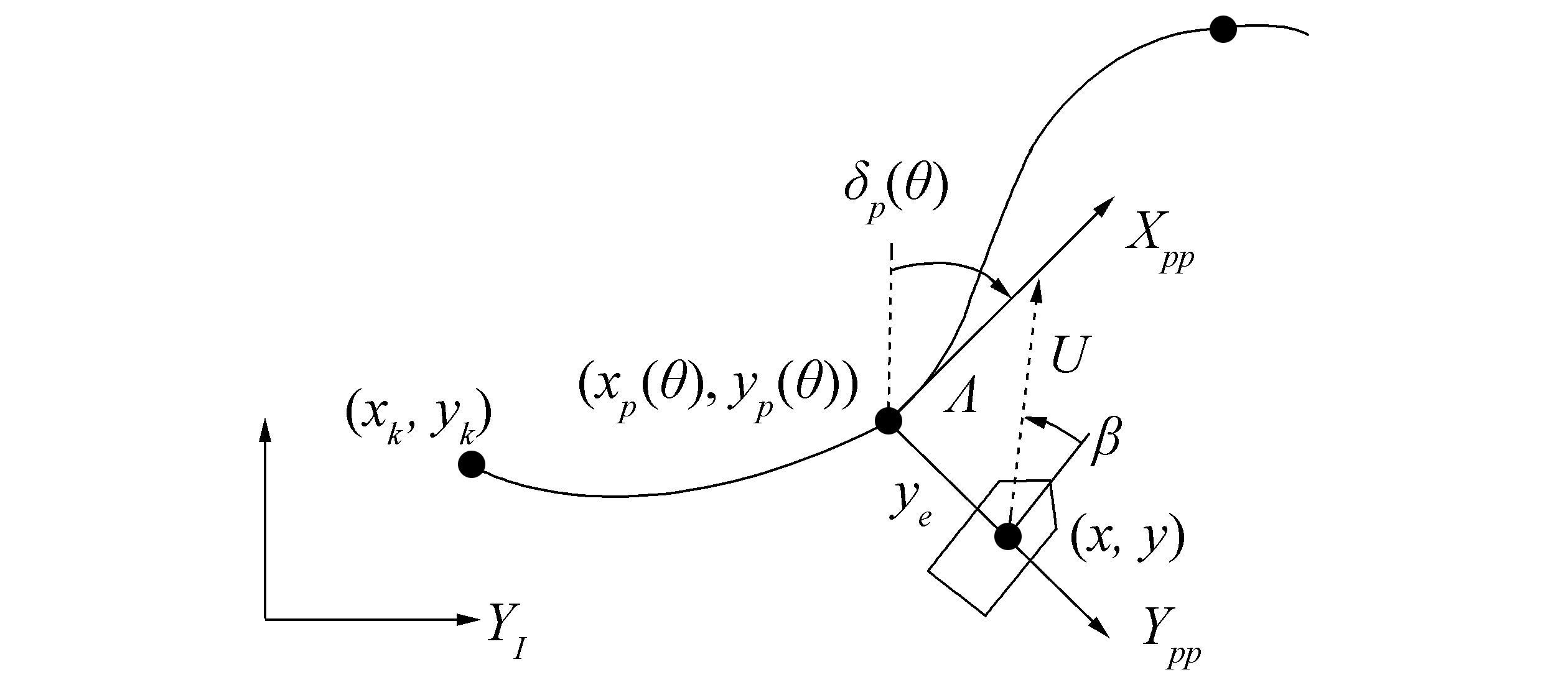
Considering that the vessel is required to converge to the path connected by a set of waypoints (xk, yk), in the horizontal plane, a Path Parallel (PP) reference frame rotated an angle δp(θ) with respect to the North-East reference frame must be used. The PP frame's origin (xp(θ), yp(θ)) lies in the path with the Xpp axis tangent to the path, as illustrated in Fig. 1.
The along-track and cross-track error for a given vessel position (x, y) can be given by
|
$\left[ {\begin{array}{*{20}{c}}
0\\
{{y_e}}
\end{array}} \right] = {\left[ {\begin{array}{*{20}{c}}
{\cos ({\delta _p}(\theta ))}&{ - \sin ({\delta _p}(\theta ))}\\
{\sin ({\delta _p}(\theta ))}&{\cos ({\delta _p}(\theta ))}
\end{array}} \right]^{\rm{T}}}\left[ {\begin{array}{*{20}{c}}
{x - {x_p}(\theta )}\\
{y - {y_p}(\theta )}
\end{array}} \right]$
|
(1) |
The rotated angle $\delta (\theta )$ can be expressed as
|
${\delta _p}(\theta ) {\rm{ = atan2(}}{\dot y_p}{\rm{(}}\theta {\rm{),}} {\dot x_p}{\rm{(}}\theta {\rm{))}}$
|
(2) |
where the two-argument function atan2 is a generalization of the arctan (y/x) function that takes into consideration both x and y in order to determine the quadrant of the result, making it possible to distinguish between opposite directions.
The normal form of Eq. (1) is given by
|
$0 = (x - {x_p}(\theta ))\cos ({\delta _p}(\theta )) + (y - {y_p}(\theta ))\sin ({\delta _p}(\theta ))$
|
(3) |
|
${y_e} = - (x - {x_p}(\theta ))\sin ({\delta _p}(\theta )) + (y - {y_p}(\theta ))\cos ({\delta _p}(\theta ))$
|
(4) |
According to Fossen (2011), the kinematic equations can be expressed as the following form,
|
$\begin{array}{l}
\dot x = u\cos (\psi ) - \upsilon \sin (\psi )\\
\dot y = u\sin (\psi ) + \upsilon \cos (\psi )\\
\dot \psi = r
\end{array}$
|
(5) |
Insert Eqs. (2), (3) and (5) into the differentiation of Eq. (4), that is
|
$\begin{array}{l}
{{\dot y}_e} = - (\dot x - {{\dot x}_p}(\theta ))\sin ({\delta _p}(\theta )) + (\dot y - {{\dot y}_p}(\theta ))\cos ({\delta _p}(\theta )) - \\
[(x - {x_p}(\theta ))\cos ({\delta _p}(\theta )) + (y - {y_p}(\theta ))\sin ({\delta _p}(\theta ))] {{\dot \delta }_p}(\theta ) = \\
- \dot x\sin ({\delta _p}(\theta )) + \dot y\cos ({\delta _p}(\theta )) = \\
- (u\cos (\psi ) - \upsilon \sin (\psi ))\sin ({\delta _p}(\theta )) + \\
{\kern 1pt} {\kern 1pt} (u\sin (\psi ) + \upsilon \cos (\psi ))\cos ({\delta _p}(\theta )) = \\
U\sin (\psi - {\delta _p}(\theta ) + \beta ) = U\sin (\chi - {\delta _p}(\theta ))
\end{array}$
|
(6) |
where χ=ψ+β is the course angle, $U = \sqrt {{u^2} + {\upsilon ^2}} $ is the horizontal speed and β=atan2(υ, u) is referred to as the sideslip angle. Commonly, the course angle can be chosen as
|
$\chi = {\delta _p}(\theta ) + \arctan \left( {\frac{{ - {y_e}}}{\mathit{\Lambda }}} \right)$
|
(7) |
Specially, a low Λ value will result in more aggressive steering comparing to a larger one. To obtain a more flexible behavior, a time-varying Λ can be implemented as (Lekkas and Fossen, 2012)
|
$\mathit{\Lambda }({y_e}) = ({\mathit{\Lambda }_{\max }} - {\mathit{\Lambda }_{\min }}){{\mathop{\rm e}\nolimits} ^{ - \mu \left| {{y_e}} \right|}} + {\mathit{\Lambda }_{\min }}$
|
(8) |
where μ is the convergence rate of Λ. If the desired heading is perfectly tracked at all time, the derivative of the cross-track error becomes
|
${\dot y_e} = U\frac{{ - {y_e}}}{{\sqrt {{\mathit{\Lambda }^2} + y_e^2} }}$
|
(9) |
Considering the Lyapunov function, $V=y_{e}^{2}/2$ and Eq. (9), the differentiation of this Lyapunov function can be given by
|
$\dot V = U\frac{{ - y_e^2}}{{\sqrt {{\mathit{\Lambda }^2} + y_e^2} }}$
|
(10) |
Eq. (10) is non-autonomous since the horizontal speed U and the look-ahead distance Λ are time-varying. For all $\forall \left| {{y_e}} \right| \le d$ and $c(d) = {U_{\min }}\sqrt {{\mathit{\Lambda }_{{{\max }^2}}} + {d^2}} $, the following can be derived,
|
$\dot V \le - 2c(d)V$
|
(11) |
Therefore, for all $t \ge {t_0}$, $\forall \left| {{y_e}} \right| \le d$ and any $d \ge 0$, Eq. (11) implies that
|
${y_e}(t) \le {{\rm{e}}^{ - c(d)(t - {t_0})}}{y_e}({t_0})$
|
(12) |
Hence, the origin ${y_e} = 0$ is a Uniform Semi-Global Exponential Stability (USGES) equilibrium of the system Eq. (9) (Fossen et al., 2014).
2.2 LOS guidance law for a straight line and a circle
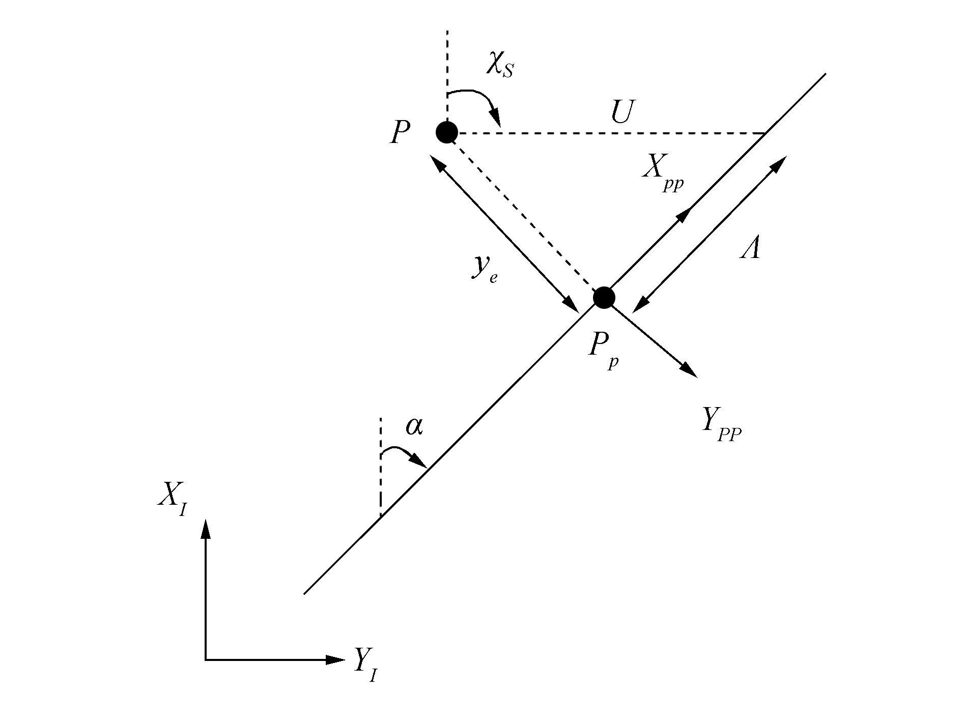
For a straight line, the PP frame is rotated an angle α relative to the inertial North-East reference frame, shown in Fig. 2. Hence, the desired heading angle can be computed as
|
${\psi _{dl}} = {\chi _s} - \beta = \alpha + \arctan \left( {\frac{{ - {y_e}}}{\mathit{\Lambda }}} \right) - \beta $
|
(13) |
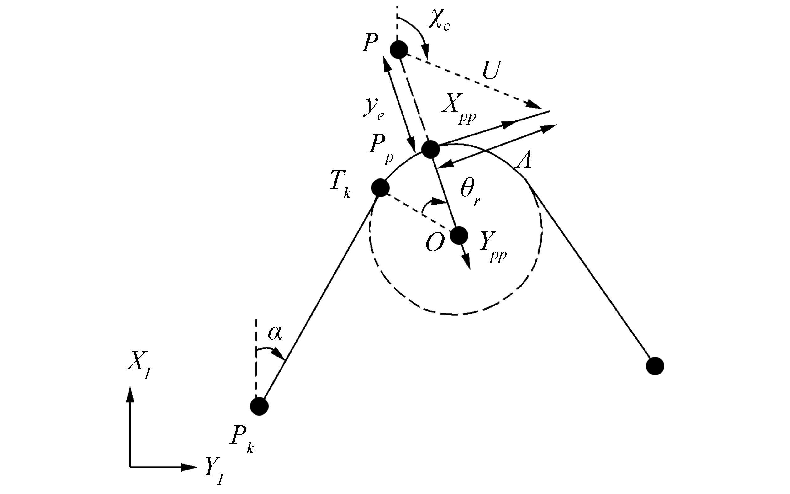
For the circle having non-zero curvature, the course angle χc is time-varying. By analyzing Fig. 3, the desired heading angle can be taken as
|
${\psi _{dc}} = {\chi _c} - \beta = \alpha + {\theta _r} + \arctan \left( {\frac{{ - {y_e}}}{\mathit{\Lambda }}} \right) - \beta $
|
(14) |
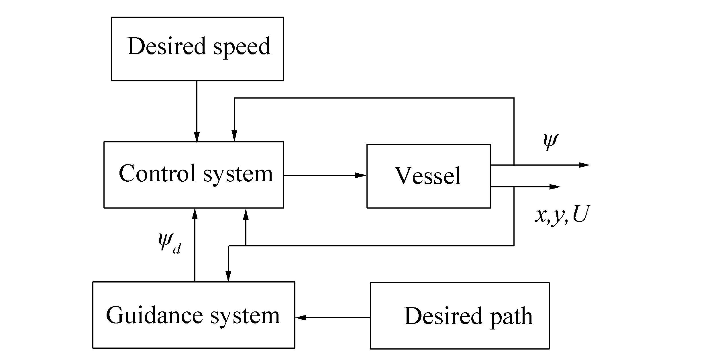
Generally, we usually assume that the sideslip angle β can be ignored compared to the heading angle ψd, that is ψd= χ. However, the course angle χ and the desired heading angle ψd will not be aligned when there exist external disturbances or during turns (Lekkas and Fossen, 2013). The guidance system is a high-level decision-making system which gives yaw command to the control system. Thus, the relationship between the guidance system and the control system can be given in Fig. 4.
3 Mathematical model
The mathematical model of path following is usually established under the assumption of port/starboard symmetry, in which only the surge, sway, and yaw motions need to be considered. In this paper, three different reference frames will be used, as shown in Fig. 5. The first, XEYEZE, is the earth-fixed frame called the North-East-Down (NED) reference frame. The second, XYZ, is a moving reference frame fixed to the body with the origin set in the midship of the water surface. The third, XDYDZD, is an earth-fixed frame called the Vessel Parallel (VP) reference frame translated to the desired position (xd, yd) and rotated to the desired heading angle ψd of the ship. The reason for keeping the VP reference frame is that the controller design will be independent of the desired position and orientation of the ship (Strand et al., 1998b).
Motivated by the actuator dynamics adopted by Morishita and Souza (2014) and Fossen and Berge (1997), a suitable mathematical model for path following can be described as (Fossen, 2011)
|
$\mathit{\boldsymbol{\dot \eta }}{\rm{ = }}\mathit{\boldsymbol{J}}(\mathit{\boldsymbol{\eta }})\mathit{\boldsymbol{v}}$
|
(15) |
|
$\mathit{\boldsymbol{M\dot v}}\mathit{ + }\mathit{\boldsymbol{Dv}}\mathit{ = }{\mathit{\boldsymbol{B}}_\mathit{u}}{\mathit{\boldsymbol{u}}_\mathit{p}}\mathit{ + }{\mathit{\boldsymbol{J}}^\mathit{T}}(\mathit{\boldsymbol{\eta }})\mathit{\boldsymbol{b}}$
|
(16) |
|
${\mathit{\boldsymbol{T}}_\mathit{u}}{{\mathit{\boldsymbol{\dot u}}}_\mathit{p}}\mathit{ + }{\mathit{\boldsymbol{u}}_\mathit{p}}\mathit{ = }{\mathit{\boldsymbol{u}}_\mathit{c}}$
|
(17) |
where $\mathit{\boldsymbol{\eta }}{\rm{ = [}}x,y,\psi {{\rm{]}}^{\rm{T}}}$ is the generalized position vector with respect to the earth-fixed frame. The body-fixed velocity is represented by the vector $\mathit{\boldsymbol{v}}{\rm{ = }}{[u,\upsilon ,r]^{\rm{T}}}$. Here J(η) is the rotation matrix; $\mathit{\boldsymbol{M}} \in {\Re ^{3 \times 3}}$ is the inertia matrix including the added inertia; $\mathit{\boldsymbol{D}} \in {\Re ^{3 \times 3}}$ is the matrix including damping coefficients; and ${\mathit{\boldsymbol{B}}_u} \in {\Re ^{3 \times n}}$ is the configuration matrix with n actuators. Also, ${\mathit{\boldsymbol{u}}_p} \in {\Re ^{n \times 1}}$ is the vector of the propeller thrusts; $\mathit{\boldsymbol{b}} \in {\Re ^{3 \times 1}}$ is the vector of the slow varying environmental forces including wind, waves, currents, and those induced by actuators; Tu is a dialogue matrix of positive time constants; and ${\mathit{\boldsymbol{u}}_c} \in {\Re ^{n \times 1}}$ is the vector of control thrusts determined by the controller.
Considering the saturation of the actuators, the control forces in surge, sway, and yaw should be limited and can be represented as
|
${\mathit{\boldsymbol{u}}_c}{\rm{ = }}\frac{1}{2}\left( {{\mathit{\boldsymbol{u}}_{{\rm{max}}}} + {\mathit{\boldsymbol{u}}_{{\rm{min}}}} - \left| {{\mathit{\boldsymbol{u}}_{{\rm{max}}}} - {\mathit{\boldsymbol{u}}_c}} \right| + \left| {{\mathit{\boldsymbol{u}}_{{\rm{min}}}} - {\mathit{\boldsymbol{u}}_c}} \right|} \right)$
|
(18) |
where ${\mathit{\boldsymbol{u}}_{{\rm{max}}}} \in {\Re ^{3 \times 1}}$ and ${\mathit{\boldsymbol{u}}_{{\rm{min}}}} \in {\Re ^{3 \times 1}}$ are the vectors with maximum and minimum saturation values, respectively. Generally, the rotation matrix J(η), inertia matrix M and damping matrix D have the following forms, respectively
|
$\mathit{\boldsymbol{J}}(\mathit{\boldsymbol{\eta }}) = \left[ {\begin{array}{*{20}{c}}
{\cos (\psi )} & { - \sin (\psi )} & 0\\
{\sin (\psi )} & {\cos (\psi )} & 0\\
0 & 0 & 1
\end{array}} \right]$
|
|
$\mathit{\boldsymbol{M}} = \left[ {\begin{array}{*{20}{c}}
{m - {X_{\dot u}}} & 0 & 0\\
0 & {m - {Y_{\dot \upsilon }}} & {m{x_g} - {Y_{\dot r}}}\\
0 & {m{x_g} - {N_{\dot \upsilon }}} & {{I_z} - {N_{\dot r}}}
\end{array}} \right]$
|
|
$\mathit{\boldsymbol{D}} = \left[ {\begin{array}{*{20}{c}}
{ - {X_u}} & 0 & 0\\
0 & { - {Y_\upsilon }} & { - {Y_r}}\\
0 & { - {N_\upsilon }} & { - {N_r}}
\end{array}} \right]$
|
4 Ship model in VP reference frame
In this section, a ship model in the VP reference frame will be established. Here the VP reference frame can be viewed as a "control-fixed" frame, where this ship model will be used to design the following controller. As the LOS guidance law can reduce the desired outputs from the desired position [xd, yd, ψd]T to the desired heading angle ψd, the deviation vector can be written as η-ηd= [0, 0, ψ-ψd]T. The deviation vector from η-ηd to the VP frame can be given as
|
$\mathit{\boldsymbol{e}} = {\mathit{\boldsymbol{J}}^{\rm{T}}}({\mathit{\boldsymbol{\eta }}_d})(\mathit{\boldsymbol{\eta }} - {\mathit{\boldsymbol{\eta }}_d})$
|
(19) |
Hence, by using the following expressions,
|
$\mathit{\boldsymbol{J}}(\mathit{\boldsymbol{e}}) = {\mathit{\boldsymbol{J}}^{\rm{T}}}({\mathit{\boldsymbol{\eta }}_d})\mathit{\boldsymbol{J}}(\mathit{\boldsymbol{\eta }})$
|
|
$\mathit{\boldsymbol{\dot J}}({\mathit{\boldsymbol{\eta }}_d}) = {r_d}\mathit{\boldsymbol{J}}({\mathit{\boldsymbol{\eta }}_d})\mathit{\boldsymbol{S}}$
|
|
$\mathit{\boldsymbol{S}} = \left[ {\begin{array}{*{20}{c}}
0 & { - 1} & 0\\
1 & 0 & 0\\
0 & 0 & 0
\end{array}} \right] = - {\mathit{\boldsymbol{S}}^{\rm{T}}}$
|
the vessel kinematic can be written as
|
$\mathit{\boldsymbol{\dot e}} = - {r_d}{\mathit{\boldsymbol{S}}^{\rm{T}}}\mathit{\boldsymbol{e}} - {\mathit{\boldsymbol{v}}_d} + \mathit{\boldsymbol{J}}(\mathit{\boldsymbol{e}})\mathit{\boldsymbol{v}}$
|
(20) |
As the main objective of path following is to follow the desired path and obtain the desired surge speed ud, the regulation of velocity can be set as vd =[ud, νd, rd]T= [ud, 0, 0]T. With the Eqs. (16) and (17), the ship model in the VP frame can be given by
|
$\mathit{\boldsymbol{\dot e}} = {\mathit{\boldsymbol{J}}_e}\mathit{\boldsymbol{v}} - {\mathit{\boldsymbol{v}}_d}$
|
(21) |
|
$\mathit{\boldsymbol{\dot v}} = - {\mathit{\boldsymbol{M}}^{ - 1}}\mathit{\boldsymbol{Dv}} + {\mathit{\boldsymbol{M}}^{ - 1}}{\mathit{\boldsymbol{B}}_\mathit{u}}{\mathit{\boldsymbol{u}}_\mathit{p}} + {\mathit{\boldsymbol{M}}^{ - 1}}\mathit{\boldsymbol{J}}_e^{\rm{T}}\mathit{\boldsymbol{J}}_d^{\rm{T}}\mathit{\boldsymbol{b}}$
|
(22) |
|
${{\mathit{\boldsymbol{\dot u}}}_p} = - \mathit{\boldsymbol{T}}_u^{ - 1}{\mathit{\boldsymbol{u}}_p} + \mathit{\boldsymbol{T}}_u^{ - 1}{\mathit{\boldsymbol{u}}_c}$
|
(23) |
where ${\mathit{\boldsymbol{J}}_e} = \mathit{\boldsymbol{J}}(\mathit{\boldsymbol{e}})$ and ${\mathit{\boldsymbol{J}}_d} = \mathit{\boldsymbol{J}}({\mathit{\boldsymbol{\eta }}_d})$.
For notational simplicity, let $\mathit{\boldsymbol{x}} = {[{\mathit{\boldsymbol{e}}^{\rm{T}}}, {\mathit{\boldsymbol{v}}^{\rm{T}}}, \mathit{\boldsymbol{u}}_p^{\rm{T}}]^{\rm{T}}}$, thus
|
$\mathit{\boldsymbol{\dot x}} = \mathit{\boldsymbol{f}}(\mathit{\boldsymbol{x}}) + \mathit{\boldsymbol{B}}{\mathit{\boldsymbol{u}}_c}$
|
(24) |
where
|
$\mathit{\boldsymbol{f}}(\mathit{\boldsymbol{x}}) = \left[ {\begin{array}{*{20}{l}}
{\quad \quad \quad \quad \quad {\mathit{\boldsymbol{J}}_e}\mathit{\boldsymbol{v}} - {\mathit{\boldsymbol{v}}_d}}\\
{ - {\mathit{\boldsymbol{M}}^{ - 1}}\mathit{\boldsymbol{Dv}} + {\mathit{\boldsymbol{M}}^{ - 1}}{\mathit{\boldsymbol{B}}_u}{\mathit{\boldsymbol{u}}_p} + {\mathit{\boldsymbol{M}}^{ - 1}}\mathit{\boldsymbol{J}}_e^{\rm{T}}\mathit{\boldsymbol{J}}_d^{\rm{T}}\mathit{\boldsymbol{b}}}\\
{\quad \quad \quad \quad \quad - \mathit{\boldsymbol{T}}_u^{ - 1}{\mathit{\boldsymbol{u}}_p}}
\end{array}} \right],\;\;\mathit{\boldsymbol{B}} = \left[ {\begin{array}{*{20}{l}}
{\;0}\\
{\;0}\\
{\mathit{\boldsymbol{T}}_u^{ - 1}}
\end{array}} \right]$
|
Eq. (24) is linearized at the desired vector x=xd, where ${\mathit{\boldsymbol{x}}_d} = {[0{\kern 1pt} {\kern 1pt} {\kern 1pt} {\kern 1pt} {\kern 1pt} {\kern 1pt} \mathit{\boldsymbol{v}}_d^{\rm{T}}{\kern 1pt} {\kern 1pt} {\kern 1pt} {\kern 1pt} {\kern 1pt} 0]^{\rm{T}}}$, that is
|
$\mathit{\boldsymbol{\dot x}} = \mathit{\boldsymbol{Ax}} + \mathit{\boldsymbol{B}}{\mathit{\boldsymbol{u}}_c}$
|
(25) |
where
|
$\mathit{\boldsymbol{A}} = {\left. {\frac{{\partial \mathit{\boldsymbol{f}}(\mathit{\boldsymbol{x}})}}{{\partial \mathit{\boldsymbol{x}}}}} \right|_{\mathit{\boldsymbol{x}} = {\mathit{\boldsymbol{x}}_d}}} = \left[ {\begin{array}{*{20}{c}}
0 & \mathit{\boldsymbol{I}} & 0\\
0 & { - {\mathit{\boldsymbol{M}}^{ - 1}}\mathit{\boldsymbol{D}}} & {{\mathit{\boldsymbol{M}}^{ - 1}}{\mathit{\boldsymbol{B}}_u}}\\
0 & 0 & { - \mathit{\boldsymbol{T}}_u^{ - 1}}
\end{array}} \right]$
|
5 Controller design
5.1 Control objectives
The control law is designed to meet one local and one global objective (Strand et al., 1998b). The local objective is to find a linear optimal control law that minimizes the cost function
|
${J_l} = \int_0^\infty {[{\mathit{\boldsymbol{x}}^{\rm{T}}}\mathit{\boldsymbol{Qx}} + \mathit{\boldsymbol{u}}_l^{\rm{T}}\mathit{\boldsymbol{R}}{\mathit{\boldsymbol{u}}_l}]} {\rm{d}}t$
|
(26) |
locally subjected to the linear system dynamic of Eq. (25) with the cost matrices Q=QT and R=RT positive definite. The global objective is to find a control law to obtain a global inverse optimality which minimizes the cost function,
|
${J_g} = \int_0^\infty {[\mathit{\boldsymbol{q}}(\mathit{\boldsymbol{x}}) + \mathit{\boldsymbol{u}}_*^{\rm{T}}{\mathit{\boldsymbol{R}}_{\bf{*}}}(\mathit{\boldsymbol{x}}){\mathit{\boldsymbol{u}}_{\rm{*}}}]} {\rm{d}}t$
|
(27) |
The global optimal control law design is an inverse approach requiring that q(x) is positive definite and ${\mathit{\boldsymbol{R}}_{\bf{*}}}(\mathit{\boldsymbol{x}}) = \mathit{\boldsymbol{R}}_{\bf{*}}^{\rm{T}}(\mathit{\boldsymbol{x}}) > 0$ to satisfy the local optimal requirements,
|
${\mathit{\boldsymbol{q}}_{xx}}({\bf{0}}) = \frac{{{\partial ^2}\mathit{\boldsymbol{q}}}}{{2\partial {\mathit{\boldsymbol{x}}^2}}} = \mathit{\boldsymbol{Q}}$
|
(28) |
5.2 Linear backstepping
The local linear control law for Eq. (26) is ${\mathit{\boldsymbol{u}}_l} = - {\mathit{\boldsymbol{R}}^{ - 1}}{\mathit{\boldsymbol{B}}^{\rm{T}}}\mathit{\boldsymbol{Px}}$, where $\mathit{\boldsymbol{P}} = {\mathit{\boldsymbol{P}}^{\rm{T}}} > 0$ can be found by solving the Generalized Algebraic Riccati Equation (GARE),
|
$\mathit{\boldsymbol{PA}} + {\mathit{\boldsymbol{A}}^{\rm{T}}}\mathit{\boldsymbol{P}} - \mathit{\boldsymbol{PB}}{\mathit{\boldsymbol{R}}^{ - 1}}{\mathit{\boldsymbol{B}}^{\rm{T}}}\mathit{\boldsymbol{P}} + \mathit{\boldsymbol{Q}} = 0$
|
(29) |
The matrix P can be factored into
|
$\mathit{\boldsymbol{P}} = {\mathit{\boldsymbol{L}}^{\rm{T}}}\mathit{\boldsymbol{ \boldsymbol{\varDelta} L}}$
|
(30) |
where Δ is a positive definite block-diagonal matrix, and L is a lower triangular matrix with identity matrices along the diagonal, namely
|
$\mathit{\boldsymbol{L}} = \left[ {\begin{array}{*{2{\bf{0}}}{c}}
\mathit{\boldsymbol{I}} & {\bf{0}} & {\bf{0}}\\
{ - {\mathit{\boldsymbol{L}}_{{\rm{11}}}}} & \mathit{\boldsymbol{I}} & {\bf{0}}\\
{ - {\mathit{\boldsymbol{L}}_{{\rm{21}}}}} & { - {\mathit{\boldsymbol{L}}_{{\rm{22}}}}} & \mathit{\boldsymbol{I}}
\end{array}} \right],\quad \mathit{\boldsymbol{ \boldsymbol{\varDelta} }} = \left[ {\begin{array}{*{2{\bf{0}}}{c}}
{{\mathit{\boldsymbol{ \boldsymbol{\varDelta} }}_{\rm{1}}}} & {\bf{0}} & {\bf{0}}\\
{\bf{0}} & {{\mathit{\boldsymbol{ \boldsymbol{\varDelta} }}_{\rm{2}}}} & {\bf{0}}\\
{\bf{0}} & {\bf{0}} & {{\mathit{\boldsymbol{ \boldsymbol{\varDelta} }}_{\rm{3}}}}
\end{array}} \right]$
|
By inserting Eq. (30) into Eq. (29), the GARE can be transformed into
|
${{\mathit{\boldsymbol{\bar A}}}^{\rm{T}}}\mathit{\boldsymbol{ \boldsymbol{\varDelta} }} + \mathit{\boldsymbol{ \boldsymbol{\varDelta} \bar A}} - \mathit{\boldsymbol{ \boldsymbol{\varDelta} B}}{\mathit{\boldsymbol{R}}^{ - 1}}{\mathit{\boldsymbol{B}}^{\rm{T}}}\mathit{\boldsymbol{ \boldsymbol{\varDelta} }} + \mathit{\boldsymbol{\bar Q}} = 0$
|
(31) |
where
|
$\mathit{\boldsymbol{\bar A}} = \mathit{\boldsymbol{LA}}{\mathit{\boldsymbol{L}}^{ - 1}} = \left[ {\begin{array}{*{2{\bf{0}}}{c}}
{{\mathit{\boldsymbol{L}}_{{\rm{11}}}}} & \mathit{\boldsymbol{I}} & {\bf{0}}\\
{{{\mathit{\boldsymbol{\bar A}}}_{{\rm{21}}}}} & {{{\mathit{\boldsymbol{\bar A}}}_{{\rm{22}}}}} & {{{\mathit{\boldsymbol{\bar A}}}_{{\rm{23}}}}}\\
{{{\mathit{\boldsymbol{\bar A}}}_{{\rm{31}}}}} & {{{\mathit{\boldsymbol{\bar A}}}_{{\rm{32}}}}} & {{{\mathit{\boldsymbol{\bar A}}}_{{\rm{33}}}}}
\end{array}} \right],$
|
|
$\mathit{\boldsymbol{\bar Q}} = {\mathit{\boldsymbol{L}}^{ - {\rm{T}}}}\mathit{\boldsymbol{Q}}{\mathit{\boldsymbol{L}}^{ - 1}} = \left[ {\begin{array}{*{20}{c}}
{{{\mathit{\boldsymbol{\bar Q}}}_{{\rm{11}}}}} & {{{\mathit{\boldsymbol{\bar Q}}}_{{\rm{12}}}}} & {{{\mathit{\boldsymbol{\bar Q}}}_{{\rm{13}}}}}\\
{{{\mathit{\boldsymbol{\bar Q}}}_{{\rm{21}}}}} & {{{\mathit{\boldsymbol{\bar Q}}}_{{\rm{22}}}}} & {{{\mathit{\boldsymbol{\bar Q}}}_{{\rm{23}}}}}\\
{{{\mathit{\boldsymbol{\bar Q}}}_{{\rm{31}}}}} & {{{\mathit{\boldsymbol{\bar Q}}}_{32}}} & {{{\mathit{\boldsymbol{\bar Q}}}_{{\rm{33}}}}}
\end{array}} \right] = {{\mathit{\boldsymbol{\bar Q}}}^{\rm{T}}}$
|
Let z be a new variable, the mapping between z and x can be written by an inverse transformation (Fossen and Strand, 1999),
|
$\mathit{\boldsymbol{z}} = \mathit{\boldsymbol{ \boldsymbol{\varPhi} }}(\mathit{\boldsymbol{x}}) = \mathit{\boldsymbol{Lx}} + \mathit{\boldsymbol{ \boldsymbol{\tilde \varPhi} }}(\mathit{\boldsymbol{x}})$
|
(32) |
where $\mathit{\boldsymbol{z}} = {[\mathit{\boldsymbol{z}}_{\rm{1}}^{\rm{T}}, \mathit{\boldsymbol{z}}_{\rm{2}}^{\rm{T}}, \mathit{\boldsymbol{z}}_{\rm{3}}^{\rm{T}}]^{\rm{T}}}$ including the linear part Lx and the nonlinear part $\mathit{\boldsymbol{ \boldsymbol{\tilde \varPhi} }}(\mathit{\boldsymbol{x}})$. Thus, the linear system, or Eq. (25) can be represented by using z=Lx,
|
${\bf{\dot z}} = \mathit{\boldsymbol{\bar Az}} + \mathit{\boldsymbol{B}}{\mathit{\boldsymbol{u}}_c}$
|
(33) |
Replacing x in ${\mathit{\boldsymbol{u}}_l} = - {\mathit{\boldsymbol{R}}^{ - 1}}{\mathit{\boldsymbol{B}}^{\rm{T}}}\mathit{\boldsymbol{Px}}$ by using z=Lx results in the following local optimal control law,
|
${\mathit{\boldsymbol{u}}_l} = - {\mathit{\boldsymbol{R}}^{ - 1}}\mathit{\boldsymbol{B \boldsymbol{\varDelta} z}}$
|
(34) |
Thus, the differentiation of the Lyapunov function $V = {\mathit{\boldsymbol{z}}^{\rm{T}}}\mathit{\boldsymbol{ \boldsymbol{\varDelta} z}}$ satisfies
|
$\dot V \le {\mathit{\boldsymbol{z}}^{\rm{T}}}\mathit{\boldsymbol{\bar Qz}} + \mathit{\boldsymbol{u}}_l^{\rm{T}}\mathit{\boldsymbol{R}}{\mathit{\boldsymbol{u}}_l}$
|
(35) |
which minimizes the cost function, namely Eq. (26).
5.3 Nonlinear backstepping
The modified inverse controller design is based on the work by Strand et al. (1998b), without the inclusion of actuator dynamics. The nonlinear inverse transformation for the model, Eqs. (21)–(23), will be performed in three steps. In the nonlinear case, the error variables can be defined as
|
${\mathit{\boldsymbol{z}}_{\rm{1}}} = \mathit{\boldsymbol{e}}$
|
(36) |
|
${\mathit{\boldsymbol{z}}_{\rm{2}}} = {\mathit{\boldsymbol{J}}_e}\mathit{\boldsymbol{v}} - {\mathit{\boldsymbol{v}}_d} - {\mathit{\boldsymbol{\alpha }}_{\rm{1}}}$
|
(37) |
|
${\mathit{\boldsymbol{z}}_{\rm{3}}} = {\mathit{\boldsymbol{u}}_p} - {\mathit{\boldsymbol{\alpha }}_{\rm{2}}}$
|
(38) |
The stabilizing vectors α1 and α2 are chosen to match the local optimality (Strand, 1999),
|
${\mathit{\boldsymbol{\alpha }}_{\rm{1}}} = {\mathit{\boldsymbol{L}}_{{\rm{11}}}}{\mathit{\boldsymbol{z}}_{\rm{1}}}$
|
(39) |
|
${\mathit{\boldsymbol{\alpha }}_{\rm{2}}} = ({\mathit{\boldsymbol{L}}_{{\rm{21}}}} + {\mathit{\boldsymbol{L}}_{{\rm{22}}}}{\mathit{\boldsymbol{L}}_{{\rm{11}}}}){\mathit{\boldsymbol{z}}_{\rm{1}}} + {\mathit{\boldsymbol{L}}_{{\rm{22}}}}{\mathit{\boldsymbol{z}}_{\rm{2}}} + {\mathit{\boldsymbol{\alpha }}_\mathit{\Gamma }} + {\mathit{\boldsymbol{\alpha }}_N}$
|
(40) |
where ${\mathit{\boldsymbol{\alpha }}_\mathit{\Gamma }}$ is the stabilizing vector induced by the slow varying environmental forces as well as the desired speed vd and αN is the stabilizing vector introduced during the controller design. Both vectors will be given in the following procedures.
Step 1: The time differentiation of Eq. (36) gives
|
${{\mathit{\boldsymbol{\dot z}}}_{\rm{1}}} = {\mathit{\boldsymbol{\alpha }}_{\rm{1}}} + ({\mathit{\boldsymbol{J}}_e}\mathit{\boldsymbol{v}} - {\mathit{\boldsymbol{v}}_d} - {\mathit{\boldsymbol{\alpha }}_{\rm{1}}})$
|
(41) |
and therefore,
|
${{\mathit{\boldsymbol{\dot z}}}_{\rm{1}}} = {\mathit{\boldsymbol{L}}_{{\rm{11}}}}{\mathit{\boldsymbol{z}}_{\rm{1}}} + {\mathit{\boldsymbol{z}}_{\rm{2}}}$
|
(42) |
Step 2: Noticing the following relationship,
|
${{\mathit{\boldsymbol{\dot J}}}_e}\mathit{\boldsymbol{J}}_e^{\rm{T}} = (r - {r_d})\mathit{\boldsymbol{S}} = r\mathit{\boldsymbol{S}}$
|
(43) |
the time differentiation of Eq. (37) with the insertion of Eqs. (22), (37)-(40), and (42)–(43) results in
|
$\begin{array}{l}
{{\mathit{\boldsymbol{\dot z}}}_{\rm{2}}} = {\mathit{\boldsymbol{J}}_e}\mathit{\boldsymbol{\dot v}} + {{\mathit{\boldsymbol{\dot J}}}_e}\mathit{\boldsymbol{v}} - {\mathit{\boldsymbol{L}}_{{\rm{11}}}}{{\mathit{\boldsymbol{\dot z}}}_{\rm{1}}} = - {\mathit{\boldsymbol{J}}_e}{\mathit{\boldsymbol{M}}^{ - 1}}\mathit{\boldsymbol{DJ}}_e^{\rm{T}}({\mathit{\boldsymbol{z}}_{\rm{2}}} + {\mathit{\boldsymbol{L}}_{{\rm{11}}}}{\mathit{\boldsymbol{z}}_{\rm{1}}} + {\mathit{\boldsymbol{v}}_d}) + \\
{\mathit{\boldsymbol{J}}_e}{\mathit{\boldsymbol{M}}^{ - 1}}{\mathit{\boldsymbol{B}}_u}\left[ {{\mathit{\boldsymbol{z}}_{\rm{3}}}{\rm{ + (}}{\mathit{\boldsymbol{L}}_{{\rm{21}}}}{\rm{ + }}{\mathit{\boldsymbol{L}}_{{\rm{22}}}}{\mathit{\boldsymbol{L}}_{{\rm{11}}}}{\rm{)}}{\mathit{\boldsymbol{z}}_{\rm{1}}} + {\mathit{\boldsymbol{L}}_{{\rm{22}}}}{\mathit{\boldsymbol{z}}_{\rm{2}}} + {\mathit{\boldsymbol{\alpha }}_\mathit{\Gamma }} + {\mathit{\boldsymbol{\alpha }}_N}} \right] + \\
{\mathit{\boldsymbol{J}}_e}{\mathit{\boldsymbol{M}}^{ - 1}}\mathit{\boldsymbol{J}}_e^{\rm{T}}\mathit{\boldsymbol{J}}_d^{\rm{T}}\mathit{\boldsymbol{b}} + r\mathit{\boldsymbol{S}}({\mathit{\boldsymbol{z}}_{\rm{2}}} + {\mathit{\boldsymbol{L}}_{{\rm{11}}}}{\mathit{\boldsymbol{z}}_{\rm{1}}} + {\mathit{\boldsymbol{v}}_d}) - {\mathit{\boldsymbol{L}}_{{\rm{11}}}}({\mathit{\boldsymbol{z}}_{\rm{2}}} + {\mathit{\boldsymbol{L}}_{{\rm{11}}}}{\mathit{\boldsymbol{z}}_{\rm{1}}})
\end{array}$
|
(44) |
To compensate for the influence of the slow varying environmental forces as well as the desired speed vd, the stabilizing vector ${\mathit{\boldsymbol{\alpha }}_\mathit{\Gamma }}$ can be chosen as
|
${\mathit{\boldsymbol{\alpha }}_\mathit{\Gamma }} = \mathit{\boldsymbol{B}}_u^ + (\mathit{\boldsymbol{DJ}}_e^{\rm{T}}{\mathit{\boldsymbol{v}}_d} - r\mathit{\boldsymbol{MJ}}_e^{\rm{T}}\mathit{\boldsymbol{S}}{\mathit{\boldsymbol{v}}_d} - \mathit{\boldsymbol{J}}_e^{\rm{T}}\mathit{\boldsymbol{J}}_d^{\rm{T}}\mathit{\boldsymbol{b}})$
|
(45) |
|
$\mathit{\boldsymbol{B}}_u^ + = \mathit{\boldsymbol{B}}_u^{\rm{T}}{({\mathit{\boldsymbol{B}}_u}\mathit{\boldsymbol{B}}_u^{\rm{T}})^{ - 1}}$
|
(46) |
By adding and subtracting the terms to obtain the linear terms ${{\mathit{\boldsymbol{\bar A}}}_{21}}{\mathit{\boldsymbol{z}}_1}$, ${{\mathit{\boldsymbol{\bar A}}}_{22}}{\mathit{\boldsymbol{z}}_2}$ and ${{\mathit{\boldsymbol{\bar A}}}_{23}}{\mathit{\boldsymbol{z}}_3}$, the expression for ${{\mathit{\boldsymbol{\dot z}}}_2}$ can be rewritten as
|
${{\mathit{\boldsymbol{\dot z}}}_2} = {{\mathit{\boldsymbol{\bar A}}}_{21}}{\mathit{\boldsymbol{z}}_1} + {{\mathit{\boldsymbol{\bar A}}}_{22}}{\mathit{\boldsymbol{z}}_2} + {{\mathit{\boldsymbol{\bar A}}}_{23}}{\mathit{\boldsymbol{z}}_3} + {\mathit{\boldsymbol{G}}_{21}}{\mathit{\boldsymbol{z}}_1} + {\mathit{\boldsymbol{G}}_{22}}{\mathit{\boldsymbol{z}}_2} + {\mathit{\boldsymbol{G}}_{23}}{\mathit{\boldsymbol{z}}_3} + {\mathit{\boldsymbol{N}}_2}$
|
(47) |
where
|
$\begin{array}{*{20}{l}}
{{\mathit{\boldsymbol{G}}_{21}} = - {\mathit{\boldsymbol{J}}_e}{\mathit{\boldsymbol{M}}^{ - 1}}\mathit{\boldsymbol{DJ}}_e^{\rm{T}}{\mathit{\boldsymbol{L}}_{11}} + {\mathit{\boldsymbol{J}}_e}{\mathit{\boldsymbol{M}}^{ - 1}}{\mathit{\boldsymbol{B}}_u}({\mathit{\boldsymbol{L}}_{21}}{\rm{ + }}{\mathit{\boldsymbol{L}}_{22}}{\mathit{\boldsymbol{L}}_{11}}) + }\\
{\quad \quad \quad \quad \quad \quad r\mathit{\boldsymbol{S}}{\mathit{\boldsymbol{L}}_{11}} - \mathit{\boldsymbol{L}}_{11}^2 - {{\mathit{\boldsymbol{\bar A}}}_{21}}}
\end{array}$
|
|
${\mathit{\boldsymbol{G}}_{22}} = - {\mathit{\boldsymbol{J}}_e}{\mathit{\boldsymbol{M}}^{ - 1}}\mathit{\boldsymbol{DJ}}_e^{\rm{T}} + {\mathit{\boldsymbol{J}}_e}{\mathit{\boldsymbol{M}}^{ - 1}}{\mathit{\boldsymbol{B}}_u}{\mathit{\boldsymbol{L}}_{22}} + r\mathit{\boldsymbol{S}} - {\mathit{\boldsymbol{L}}_{11}} - {\mathit{\boldsymbol{\bar A}}_{22}}$
|
|
${\mathit{\boldsymbol{G}}_{23}} = {\mathit{\boldsymbol{J}}_e}{\mathit{\boldsymbol{M}}^{ - 1}}{\mathit{\boldsymbol{B}}_u} - {{\mathit{\boldsymbol{\bar A}}}_{23}}$
|
|
${\mathit{\boldsymbol{N}}_2} = {\mathit{\boldsymbol{J}}_e}{\mathit{\boldsymbol{M}}^{ - 1}}{\mathit{\boldsymbol{B}}_u}{\mathit{\boldsymbol{\alpha }}_N}$
|
Step 3: The time differentiation of Eq. (38) with the insertion of Eqs. (23), (38), (40), (42), and (47) results in
|
$\begin{array}{l}
{{\mathit{\boldsymbol{\dot z}}}_3} = - \mathit{\boldsymbol{T}}_u^{ - 1}{\mathit{\boldsymbol{u}}_p} + \mathit{\boldsymbol{T}}_u^{ - 1}{\mathit{\boldsymbol{u}}_c} - {{\mathit{\boldsymbol{\dot \alpha }}}_2} = \\
\mathit{\boldsymbol{T}}_u^{ - 1}{\mathit{\boldsymbol{u}}_c} - {\rm{(}}{\mathit{\boldsymbol{L}}_{21}}{\rm{ + }}{\mathit{\boldsymbol{L}}_{22}}{\mathit{\boldsymbol{L}}_{11}}{\rm{)(}}{\mathit{\boldsymbol{z}}_2} + {\mathit{\boldsymbol{L}}_{11}}{\mathit{\boldsymbol{z}}_1}) - \\
{\kern 1pt} \mathit{\boldsymbol{T}}_u^{ - 1}\left[ {{\mathit{\boldsymbol{z}}_3}{\rm{ + (}}{\mathit{\boldsymbol{L}}_{21}}{\rm{ + }}{\mathit{\boldsymbol{L}}_{22}}{\mathit{\boldsymbol{L}}_{11}}{\rm{)}}{\mathit{\boldsymbol{z}}_1} + {\mathit{\boldsymbol{L}}_{22}}{\mathit{\boldsymbol{z}}_2} + {\mathit{\boldsymbol{\alpha }}_\mathit{\Gamma }} + {\mathit{\boldsymbol{\alpha }}_N}} \right]{\kern 1pt} {\kern 1pt} - \\
{\mathit{\boldsymbol{L}}_{22}}({{\mathit{\boldsymbol{\bar A}}}_{21}}{\mathit{\boldsymbol{z}}_1} + {{\mathit{\boldsymbol{\bar A}}}_{22}}{\mathit{\boldsymbol{z}}_2} + {{\mathit{\boldsymbol{\bar A}}}_{23}}{\mathit{\boldsymbol{z}}_3} + {\mathit{\boldsymbol{G}}_{21}}{\mathit{\boldsymbol{z}}_1} + {\mathit{\boldsymbol{G}}_{22}}{\mathit{\boldsymbol{z}}_2} + \\
{\kern 1pt} {\mathit{\boldsymbol{G}}_{23}}{\mathit{\boldsymbol{z}}_3} + {\mathit{\boldsymbol{N}}_2}) - {{\mathit{\boldsymbol{\dot \alpha }}}_\mathit{\Gamma }} - {{\mathit{\boldsymbol{\dot \alpha }}}_N}
\end{array}$
|
(48) |
The expression for ${{\mathit{\boldsymbol{\dot z}}}_3}$ can be rewritten in a similar manner by adding and subtracting the terms ${{\mathit{\boldsymbol{\bar A}}}_{31}}{\mathit{\boldsymbol{z}}_1}$, ${{\mathit{\boldsymbol{\bar A}}}_{32}}{\mathit{\boldsymbol{z}}_2}$ and ${{\mathit{\boldsymbol{\bar A}}}_{33}}{\mathit{\boldsymbol{z}}_3}$,
|
$\begin{array}{l}
{{\mathit{\boldsymbol{\dot z}}}_3} = {{\mathit{\boldsymbol{\bar A}}}_{31}}{\mathit{\boldsymbol{z}}_1} + {{\mathit{\boldsymbol{\bar A}}}_{32}}{\mathit{\boldsymbol{z}}_2} + {{\mathit{\boldsymbol{\bar A}}}_{33}}{\mathit{\boldsymbol{z}}_3} + {\mathit{\boldsymbol{G}}_{31}}{\mathit{\boldsymbol{z}}_1} + \\
{\kern 1pt} {\kern 1pt} {\kern 1pt} {\kern 1pt} {\kern 1pt} {\kern 1pt} {\kern 1pt} {\kern 1pt} {\kern 1pt} {\kern 1pt} {\kern 1pt} {\kern 1pt} {\kern 1pt} {\kern 1pt} {\kern 1pt} {\kern 1pt} {\kern 1pt} {\mathit{\boldsymbol{G}}_{32}}{\mathit{\boldsymbol{z}}_2} + {\mathit{\boldsymbol{G}}_{33}}{\mathit{\boldsymbol{z}}_3} + \mathit{\boldsymbol{T}}_u^{ - 1}{\mathit{\boldsymbol{u}}_c} + {\mathit{\boldsymbol{ \boldsymbol{\varGamma} }}_3} + {\mathit{\boldsymbol{N}}_3}
\end{array}$
|
(49) |
where
|
$\begin{array}{l}
{\mathit{\boldsymbol{G}}_{31}} = - \mathit{\boldsymbol{T}}_u^{ - 1}{\rm{(}}{\mathit{\boldsymbol{L}}_{21}}{\rm{ + }}{\mathit{\boldsymbol{L}}_{22}}{\mathit{\boldsymbol{L}}_{11}}{\rm{)}} - {\rm{(}}{\mathit{\boldsymbol{L}}_{21}}{\rm{ + }}{\mathit{\boldsymbol{L}}_{22}}{\mathit{\boldsymbol{L}}_{11}}{\rm{)}}{\mathit{\boldsymbol{L}}_{11}} - \\
{\kern 1pt} {\kern 1pt} {\kern 1pt} {\kern 1pt} {\kern 1pt} {\kern 1pt} {\kern 1pt} {\kern 1pt} {\kern 1pt} {\kern 1pt} {\kern 1pt} {\kern 1pt} {\kern 1pt} {\kern 1pt} {\kern 1pt} {\kern 1pt} {\kern 1pt} {\kern 1pt} {\kern 1pt} {\kern 1pt} {\kern 1pt} {\kern 1pt} {\kern 1pt} {\mathit{\boldsymbol{L}}_{22}}{{\mathit{\boldsymbol{\bar A}}}_{21}} - {\mathit{\boldsymbol{L}}_{22}}{\mathit{\boldsymbol{G}}_{21}} - {{\mathit{\boldsymbol{\bar A}}}_{31}}
\end{array}$
|
|
$\begin{array}{l}
{\mathit{\boldsymbol{G}}_{32}} = - \mathit{\boldsymbol{T}}_u^{ - 1}{\mathit{\boldsymbol{L}}_{22}} - {\rm{(}}{\mathit{\boldsymbol{L}}_{21}}{\rm{ + }}{\mathit{\boldsymbol{L}}_{22}}{\mathit{\boldsymbol{L}}_{11}}{\rm{)}} - \\
{\kern 1pt} {\kern 1pt} {\kern 1pt} {\kern 1pt} {\kern 1pt} {\kern 1pt} {\kern 1pt} {\kern 1pt} {\kern 1pt} {\kern 1pt} {\kern 1pt} {\kern 1pt} {\kern 1pt} {\kern 1pt} {\kern 1pt} {\kern 1pt} {\kern 1pt} {\kern 1pt} {\kern 1pt} {\kern 1pt} {\kern 1pt} {\kern 1pt} {\kern 1pt} {\mathit{\boldsymbol{L}}_{22}}{{\mathit{\boldsymbol{\bar A}}}_{22}} - {\mathit{\boldsymbol{L}}_{22}}{\mathit{\boldsymbol{G}}_{22}} - {{\mathit{\boldsymbol{\bar A}}}_{32}}
\end{array}$
|
|
${\mathit{\boldsymbol{ \boldsymbol{\varGamma} }}_3} = - \mathit{\boldsymbol{T}}_u^{ - 1}{\mathit{\boldsymbol{\alpha }}_\mathit{\Gamma }} - {{\mathit{\boldsymbol{\dot \alpha }}}_\mathit{\Gamma }}$
|
|
${\mathit{\boldsymbol{N}}_3} = - \mathit{\boldsymbol{T}}_u^{ - 1}{\mathit{\boldsymbol{\alpha }}_N} - {{\mathit{\boldsymbol{\dot \alpha }}}_N}$
|
Thus, the nonlinear system, Eq. (24) can be transformed into a new mapping,
|
$\mathit{\boldsymbol{\dot z}} = \mathit{\boldsymbol{\bar Az}} + \mathit{\boldsymbol{B}}{\mathit{\boldsymbol{u}}_c} + \mathit{\boldsymbol{Gz}} + \mathit{\boldsymbol{ \boldsymbol{\varGamma} }} + \mathit{\boldsymbol{N}}$
|
(50) |
where
|
$\mathit{\boldsymbol{G}} = \left[ {\begin{array}{*{2{\bf{0}}}{c}}
{\bf{0}} & {\bf{0}} & {\bf{0}}\\
{{\mathit{\boldsymbol{G}}_{21}}} & {{\mathit{\boldsymbol{G}}_{22}}} & {{\mathit{\boldsymbol{G}}_{23}}}\\
{{\mathit{\boldsymbol{G}}_{31}}} & {{\mathit{\boldsymbol{G}}_{32}}} & {{\mathit{\boldsymbol{G}}_{33}}}
\end{array}} \right],\quad \mathit{\boldsymbol{ \boldsymbol{\varGamma} }}{\rm{ = }}\left[ {\begin{array}{*{2{\bf{0}}}{c}}
{\bf{0}}\\
{\bf{0}}\\
{{\mathit{\boldsymbol{ \boldsymbol{\varGamma} }}_3}}
\end{array}} \right],\quad \mathit{\boldsymbol{N}}{\rm{ = }}\left[ {\begin{array}{*{2{\bf{0}}}{c}}
{\bf{0}}\\
{{\mathit{\boldsymbol{N}}_2}}\\
{{\mathit{\boldsymbol{N}}_3}}
\end{array}} \right]$
|
5.4 Local and global optimal controller design
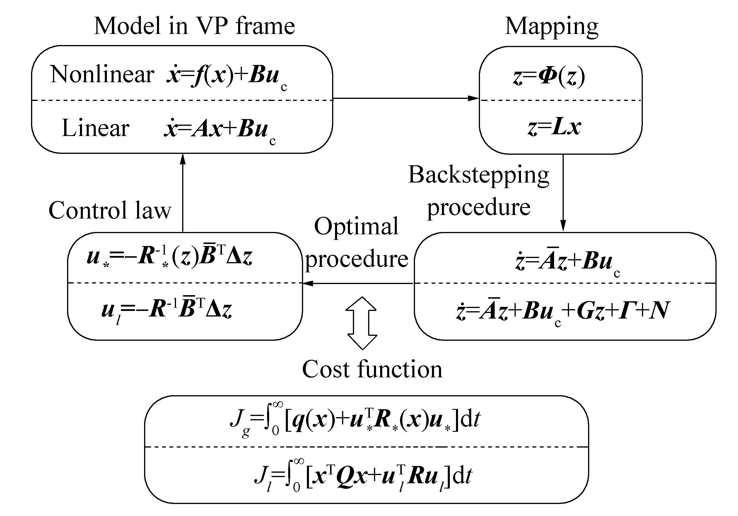
Our objective is to design a stable nonlinear state feedback controller, whose linear part is the same as the linear optimal controller in Eq. (34). The control system block diagram is given in Fig. 6.
Let the Lyapunov function be chosen as
|
$V = {\mathit{\boldsymbol{z}}^{\rm{T}}}\mathit{\boldsymbol{ \boldsymbol{\varDelta} z}} + {{\mathit{\boldsymbol{\tilde b}}}^{\rm{T}}}{\mathit{\boldsymbol{ \boldsymbol{\varOmega} }}^{ - 1}}\mathit{\boldsymbol{\tilde b}}$
|
(51) |
where $\mathit{\boldsymbol{\tilde b}} \in {\Re ^{3 \times 1}}$ is the adaptation error defined as $\mathit{\boldsymbol{\tilde b}} = \mathit{\boldsymbol{b}} - \mathit{\boldsymbol{\tilde b}}$ with ${\mathit{\boldsymbol{\hat b}}}$ being the estimate of the slow varying environmental forces b and $\mathit{\boldsymbol{ \boldsymbol{\varOmega} }} = {\mathit{\boldsymbol{ \boldsymbol{\varOmega} }}^{\rm{T}}} > 0$ is the gain matrix.
Assuming that $\mathit{\boldsymbol{\dot b}} = 0$, the differentiation of Eq. (51) gives
|
$\begin{array}{l}
\dot V = {\mathit{\boldsymbol{z}}^{\rm{T}}}({{\mathit{\boldsymbol{\bar A}}}^{\rm{T}}}\mathit{\boldsymbol{ \boldsymbol{\varDelta} }}{\bf{ + }}\mathit{\boldsymbol{ \boldsymbol{\varDelta} \bar A}})\mathit{\boldsymbol{z}} + \\
{\kern 1pt} {\kern 1pt} {\kern 1pt} {\kern 1pt} {\kern 1pt} {\kern 1pt} {\kern 1pt} {\kern 1pt} {\kern 1pt} {\kern 1pt} {\kern 1pt} {\kern 1pt} {\kern 1pt} {\kern 1pt} {\kern 1pt} {\kern 1pt} 2\mathit{\boldsymbol{z}}_2^{\rm{T}}{\mathit{\boldsymbol{ \boldsymbol{\varDelta} }}_2}({\mathit{\boldsymbol{G}}_{21}}{\mathit{\boldsymbol{z}}_1} + {\mathit{\boldsymbol{G}}_{22}}{\mathit{\boldsymbol{z}}_2} + {\mathit{\boldsymbol{G}}_{23}}{\mathit{\boldsymbol{z}}_3} + {\mathit{\boldsymbol{N}}_2}) + \\
{\kern 1pt} {\kern 1pt} {\kern 1pt} {\kern 1pt} {\kern 1pt} {\kern 1pt} {\kern 1pt} {\kern 1pt} {\kern 1pt} {\kern 1pt} {\kern 1pt} {\kern 1pt} {\kern 1pt} {\kern 1pt} {\kern 1pt} {\kern 1pt} 2\mathit{\boldsymbol{z}}_3^{\rm{T}}{\mathit{\boldsymbol{ \boldsymbol{\varDelta} }}_3}\left[ {{\mathit{\boldsymbol{G}}_{31}}{\mathit{\boldsymbol{z}}_1} + {\mathit{\boldsymbol{G}}_{32}}{\mathit{\boldsymbol{z}}_2} + {\mathit{\boldsymbol{G}}_{33}}{\mathit{\boldsymbol{z}}_3} + } \right.\\
{\kern 1pt} {\kern 1pt} {\kern 1pt} {\kern 1pt} {\kern 1pt} {\kern 1pt} {\kern 1pt} {\kern 1pt} {\kern 1pt} {\kern 1pt} {\kern 1pt} {\kern 1pt} {\kern 1pt} {\kern 1pt} {\kern 1pt} {\kern 1pt} \left. {\mathit{\boldsymbol{T}}_u^{ - 1}({\mathit{\boldsymbol{u}}_c} + {\mathit{\boldsymbol{T}}_u}{{\mathit{\boldsymbol{ \boldsymbol{\hat \varGamma} }}}_3} + {\mathit{\boldsymbol{T}}_u}{\mathit{\boldsymbol{N}}_3})} \right] + \\
{\kern 1pt} {\kern 1pt} {\kern 1pt} {\kern 1pt} {\kern 1pt} {\kern 1pt} {\kern 1pt} {\kern 1pt} {\kern 1pt} {\kern 1pt} {\kern 1pt} {\kern 1pt} {\kern 1pt} {\kern 1pt} {\kern 1pt} {\kern 1pt} 2{{\mathit{\boldsymbol{\tilde b}}}^{\rm{T}}}\left[ {{\mathit{\boldsymbol{J}}_d}{\mathit{\boldsymbol{J}}_e}{{(\mathit{\boldsymbol{B}}_u^ + )}^{\rm{T}}}\mathit{\boldsymbol{T}}_u^{ - {\rm{T}}}{\mathit{\boldsymbol{ \boldsymbol{\varDelta} }}_3}{\mathit{\boldsymbol{z}}_3} - {\mathit{\boldsymbol{ \boldsymbol{\varOmega} }}^{ - 1}}{\mathit{\boldsymbol{\dot{\hat{b}}}}}} \right]
\end{array}$
|
(52) |
where ${{\mathit{\boldsymbol{ \boldsymbol{\hat \varGamma} }}}_3}$ is the estimation of Γ3 with elements b replaced by ${\mathit{\boldsymbol{\hat b}}}$ in Eq. (45). For notational simplicity, let ${\mathit{\boldsymbol{u}}_*} = {\mathit{\boldsymbol{u}}_c} + {\mathit{\boldsymbol{T}}_u}{{\mathit{\boldsymbol{ \boldsymbol{\hat \varGamma} }}}_3} + {\mathit{\boldsymbol{T}}_u}{\mathit{\boldsymbol{N}}_3}$ and the integral action of ${\mathit{\boldsymbol{\hat b}}}$ can be chosen as
|
${\mathit{\boldsymbol{\dot{\hat{b}}}}} = \mathit{\boldsymbol{ \boldsymbol{\varOmega} }}{\mathit{\boldsymbol{J}}_d}{\mathit{\boldsymbol{J}}_e}{(\mathit{\boldsymbol{B}}_u^ + )^{\rm{T}}}\mathit{\boldsymbol{T}}_u^{ - {\rm{T}}}{\mathit{\boldsymbol{ \boldsymbol{\varDelta} }}_3}{\mathit{\boldsymbol{z}}_3}$
|
(53) |
Insert Eqs. (31) and (53) into Eq. (52) to yield
|
$\begin{array}{l}
\dot V = - {\mathit{\boldsymbol{z}}^{\rm{T}}}\mathit{\boldsymbol{\bar Qz}} + \mathit{\boldsymbol{z}}_3^{\rm{T}}{\mathit{\boldsymbol{ \boldsymbol{\varDelta} }}_3}\mathit{\boldsymbol{T}}_u^{ - 1}{\mathit{\boldsymbol{R}}^{ - 1}}\mathit{\boldsymbol{T}}_u^{ - {\rm{T}}}{\mathit{\boldsymbol{ \boldsymbol{\varDelta} }}_3}{\mathit{\boldsymbol{z}}_3} + \\
2\mathit{\boldsymbol{z}}_2^{\rm{T}}{\mathit{\boldsymbol{ \boldsymbol{\varDelta} }}_2}({\mathit{\boldsymbol{G}}_{21}}{\mathit{\boldsymbol{z}}_1} + {\mathit{\boldsymbol{G}}_{22}}{\mathit{\boldsymbol{z}}_2} + {\mathit{\boldsymbol{G}}_{23}}{\mathit{\boldsymbol{z}}_3} + {\mathit{\boldsymbol{N}}_2}) + \\
2\mathit{\boldsymbol{z}}_3^{\rm{T}}{\mathit{\boldsymbol{ \boldsymbol{\varDelta} }}_3}({\mathit{\boldsymbol{G}}_{31}}{\mathit{\boldsymbol{z}}_1} + {\mathit{\boldsymbol{G}}_{32}}{\mathit{\boldsymbol{z}}_2} + {\mathit{\boldsymbol{G}}_{33}}{\mathit{\boldsymbol{z}}_3} + \mathit{\boldsymbol{T}}_u^{ - 1}{\mathit{\boldsymbol{u}}_{\bf{*}}})
\end{array}$
|
(54) |
With the property $\mathit{\boldsymbol{\bar Q}} = {{\mathit{\boldsymbol{\bar Q}}}^{\rm{T}}}$, the expression $ - {\mathit{\boldsymbol{z}}^{\rm{T}}}\mathit{\boldsymbol{\bar Qz}}$ can be rewritten as
|
$\begin{array}{l}
- {\mathit{\boldsymbol{z}}^{\rm{T}}}\mathit{\boldsymbol{\bar Qz}} = - \mathit{\boldsymbol{z}}_1^{\rm{T}}{{\mathit{\boldsymbol{\bar Q}}}_{11}}{\mathit{\boldsymbol{z}}_1} - \mathit{\boldsymbol{z}}_2^{\rm{T}}{{\mathit{\boldsymbol{\bar Q}}}_{22}}{\mathit{\boldsymbol{z}}_2} - \mathit{\boldsymbol{z}}_3^{\rm{T}}{{\mathit{\boldsymbol{\bar Q}}}_{33}}{\mathit{\boldsymbol{z}}_3} - \\
{\kern 1pt} {\kern 1pt} {\kern 1pt} {\kern 1pt} {\kern 1pt} {\kern 1pt} {\kern 1pt} {\kern 1pt} {\kern 1pt} {\kern 1pt} {\kern 1pt} 2\mathit{\boldsymbol{z}}_2^{\rm{T}}{{\mathit{\boldsymbol{\bar Q}}}_{21}}{\mathit{\boldsymbol{z}}_1} - 2\mathit{\boldsymbol{z}}_3^{\rm{T}}{{\mathit{\boldsymbol{\bar Q}}}_{31}}{\mathit{\boldsymbol{z}}_1} - 2\mathit{\boldsymbol{z}}_3^{\rm{T}}{{\mathit{\boldsymbol{\bar Q}}}_{32}}{\mathit{\boldsymbol{z}}_2}
\end{array}$
|
(55) |
First, complete the squares for
|
$\begin{array}{l}
2\mathit{\boldsymbol{z}}_2^{\rm{T}}{\mathit{\boldsymbol{ \boldsymbol{\varDelta} }}_2}{\mathit{\boldsymbol{N}}_2} = - \mathit{\boldsymbol{N}}_2^{\rm{T}}{\mathit{\boldsymbol{R}}_N}{\mathit{\boldsymbol{N}}_2} + \left\| {{\mathit{\boldsymbol{N}}_2}{\rm{ + }}\mathit{\boldsymbol{R}}_N^{ - 1}{\mathit{\boldsymbol{ \boldsymbol{\varDelta} }}_2}{\mathit{\boldsymbol{z}}_2}} \right\|_{{\mathit{\boldsymbol{R}}_N}}^{\bf{2}} - \\
{\kern 1pt} {\kern 1pt} {\kern 1pt} {\kern 1pt} {\kern 1pt} {\kern 1pt} {\kern 1pt} {\kern 1pt} {\kern 1pt} {\kern 1pt} {\kern 1pt} {\kern 1pt} {\kern 1pt} {\kern 1pt} {\kern 1pt} {\kern 1pt} {\kern 1pt} {\kern 1pt} {\kern 1pt} {\kern 1pt} {\kern 1pt} {\kern 1pt} {\kern 1pt} {\kern 1pt} {\kern 1pt} {\kern 1pt} {\kern 1pt} {\kern 1pt} {\kern 1pt} {\kern 1pt} {\kern 1pt} {\kern 1pt} {\kern 1pt} {\kern 1pt} {\kern 1pt} {\kern 1pt} {\kern 1pt} {\kern 1pt} {\kern 1pt} {\kern 1pt} {\kern 1pt} {\kern 1pt} {\kern 1pt} \mathit{\boldsymbol{z}}_2^{\rm{T}}{\mathit{\boldsymbol{ \boldsymbol{\varDelta} }}_2}\mathit{\boldsymbol{R}}_N^{ - {\rm{T}}}{\mathit{\boldsymbol{ \boldsymbol{\varDelta} }}_2}{\mathit{\boldsymbol{z}}_2}
\end{array}$
|
(56) |
|
$\begin{array}{l}
2\mathit{\boldsymbol{z}}_3^{\rm{T}}{\mathit{\boldsymbol{ \boldsymbol{\varDelta} }}_3}\mathit{\boldsymbol{T}}_u^{ - 1}{\mathit{\boldsymbol{u}}_*} = - \mathit{\boldsymbol{u}}_{\bf{*}}^{\rm{T}}{\mathit{\boldsymbol{R}}_{\bf{*}}}{\mathit{\boldsymbol{u}}_{\bf{*}}} + \left\| {{\mathit{\boldsymbol{u}}_{\bf{*}}}{\rm{ + }}\mathit{\boldsymbol{R}}_{\bf{*}}^{ - 1}\mathit{\boldsymbol{T}}_u^{ - {\rm{T}}}{\mathit{\boldsymbol{ \boldsymbol{\varDelta} }}_3}{\mathit{\boldsymbol{z}}_3}} \right\|_{{\mathit{\boldsymbol{R}}_{\bf{*}}}}^{\bf{2}} - \\
{\kern 1pt} {\kern 1pt} {\kern 1pt} {\kern 1pt} {\kern 1pt} {\kern 1pt} {\kern 1pt} {\kern 1pt} {\kern 1pt} {\kern 1pt} {\kern 1pt} {\kern 1pt} {\kern 1pt} {\kern 1pt} {\kern 1pt} {\kern 1pt} {\kern 1pt} {\kern 1pt} {\kern 1pt} {\kern 1pt} {\kern 1pt} {\kern 1pt} {\kern 1pt} {\kern 1pt} {\kern 1pt} {\kern 1pt} {\kern 1pt} {\kern 1pt} {\kern 1pt} {\kern 1pt} {\kern 1pt} {\kern 1pt} {\kern 1pt} {\kern 1pt} {\kern 1pt} {\kern 1pt} {\kern 1pt} {\kern 1pt} {\kern 1pt} {\kern 1pt} {\kern 1pt} {\kern 1pt} {\kern 1pt} {\kern 1pt} {\kern 1pt} {\kern 1pt} {\kern 1pt} \mathit{\boldsymbol{z}}_3^{\rm{T}}{\mathit{\boldsymbol{ \boldsymbol{\varDelta} }}_3}\mathit{\boldsymbol{T}}_u^{ - 1}\mathit{\boldsymbol{R}}_{\bf{*}}^{ - {\rm{T}}}\mathit{\boldsymbol{T}}_u^{ - {\rm{T}}}{\mathit{\boldsymbol{ \boldsymbol{\varDelta} }}_3}{\mathit{\boldsymbol{z}}_3}
\end{array}$
|
(57) |
Then, the term $\mathit{\boldsymbol{z}}_1^{\rm{T}}{{\mathit{\boldsymbol{\bar Q}}}_{11}}{\mathit{\boldsymbol{z}}_1}$ will be split into ${\varepsilon _1}\mathit{\boldsymbol{z}}_1^{\rm{T}}{{\mathit{\boldsymbol{\bar Q}}}_{11}}{\mathit{\boldsymbol{z}}_1}$ and $(1 - {\varepsilon _1})\mathit{\boldsymbol{z}}_1^{\rm{T}}{{\mathit{\boldsymbol{\bar Q}}}_{11}}{\mathit{\boldsymbol{z}}_1}$ to complete the squares for
|
$\begin{array}{l}
- (1 - {\varepsilon _1})\mathit{\boldsymbol{z}}_1^{\rm{T}}{{\mathit{\boldsymbol{\bar Q}}}_{11}}{\mathit{\boldsymbol{z}}_1} - 2\mathit{\boldsymbol{z}}_2^{\rm{T}}({{\mathit{\boldsymbol{\bar Q}}}_{21}} - {\mathit{\boldsymbol{ \boldsymbol{\varDelta} }}_2}{\mathit{\boldsymbol{G}}_{21}}){\mathit{\boldsymbol{z}}_1} = \\
- \left\| {{\mathit{\boldsymbol{z}}_{\bf{1}}} + \frac{1}{{1 - {\varepsilon _1}}}\mathit{\boldsymbol{\bar Q}}_{11}^{ - 1}({{\mathit{\boldsymbol{\bar Q}}}_{12}} - \mathit{\boldsymbol{G}}_{21}^{\rm{T}}{\mathit{\boldsymbol{ \boldsymbol{\varDelta} }}_2}){\mathit{\boldsymbol{z}}_2}} \right\|_{(1 - {\varepsilon _1}){{\mathit{\boldsymbol{\bar Q}}}_{11}}}^2 + \\
{\kern 1pt} {\kern 1pt} \frac{1}{{1 - {\varepsilon _1}}}\mathit{\boldsymbol{z}}_2^{\rm{T}}{{\mathit{\boldsymbol{\bar Q}}}_{21}}\mathit{\boldsymbol{\bar Q}}_{11}^{ - {\rm{T}}}{{\mathit{\boldsymbol{\bar Q}}}_{12}}{\mathit{\boldsymbol{z}}_2}{\kern 1pt} - {\kern 1pt} \frac{1}{{1 - {\varepsilon _1}}}\mathit{\boldsymbol{z}}_2^{\rm{T}}{{\mathit{\boldsymbol{\bar Q}}}_{21}}\mathit{\boldsymbol{\bar Q}}_{11}^{ - {\rm{T}}}{{\mathit{\boldsymbol{\bar Q}}}_{12}}{\mathit{\boldsymbol{z}}_2} + \\
{\kern 1pt} {\kern 1pt} \frac{1}{{1 - {\varepsilon _1}}}\mathit{\boldsymbol{z}}_2^{\rm{T}}({{\mathit{\boldsymbol{\bar Q}}}_{21}} - {\mathit{\boldsymbol{ \boldsymbol{\varDelta} }}_2}{\mathit{\boldsymbol{G}}_{21}})\mathit{\boldsymbol{\bar Q}}_{11}^{ - {\rm{T}}}({{\mathit{\boldsymbol{\bar Q}}}_{12}} - \mathit{\boldsymbol{G}}_{21}^{\rm{T}}{\mathit{\boldsymbol{ \boldsymbol{\varDelta} }}_2}){\mathit{\boldsymbol{z}}_2}{\kern 1pt}
\end{array}$
|
(58) |
|
$\begin{array}{l}
- {\varepsilon _1}\mathit{\boldsymbol{z}}_1^{\rm{T}}{{\mathit{\boldsymbol{\bar Q}}}_{11}}{\mathit{\boldsymbol{z}}_1} - 2\mathit{\boldsymbol{z}}_3^{\rm{T}}({{\mathit{\boldsymbol{\bar Q}}}_{31}} - {\mathit{\boldsymbol{ \boldsymbol{\varDelta} }}_3}{\mathit{\boldsymbol{G}}_{31}}){\mathit{\boldsymbol{z}}_1} = \\
- \left\| {{\mathit{\boldsymbol{z}}_1} + \frac{1}{{{\varepsilon _1}}}\mathit{\boldsymbol{\bar Q}}_{11}^{ - 1}({{\mathit{\boldsymbol{\bar Q}}}_{13}} - \mathit{\boldsymbol{G}}_{31}^{\rm{T}}{\mathit{\boldsymbol{ \boldsymbol{\varDelta} }}_3}){\mathit{\boldsymbol{z}}_3}} \right\|_{{\varepsilon _1}{{\mathit{\boldsymbol{\bar Q}}}_{11}}}^2 + \\
\frac{1}{{{\varepsilon _1}}}\mathit{\boldsymbol{z}}_3^{\rm{T}}{{\mathit{\boldsymbol{\bar Q}}}_{31}}\mathit{\boldsymbol{\bar Q}}_{11}^{ - {\rm{T}}}{{\mathit{\boldsymbol{\bar Q}}}_{13}}{\mathit{\boldsymbol{z}}_3} - \frac{1}{{{\varepsilon _1}}}\mathit{\boldsymbol{z}}_3^{\rm{T}}{{\mathit{\boldsymbol{\bar Q}}}_{31}}\mathit{\boldsymbol{\bar Q}}_{11}^{ - {\rm{T}}}{{\mathit{\boldsymbol{\bar Q}}}_{13}}{\mathit{\boldsymbol{z}}_3} + \\
\frac{1}{{{\varepsilon _1}}}\mathit{\boldsymbol{z}}_3^{\rm{T}}({{\mathit{\boldsymbol{\bar Q}}}_{31}} - {\mathit{\boldsymbol{ \boldsymbol{\varDelta} }}_3}{\mathit{\boldsymbol{G}}_{31}})\mathit{\boldsymbol{\bar Q}}_{11}^{ - {\rm{T}}}({{\mathit{\boldsymbol{\bar Q}}}_{13}} - \mathit{\boldsymbol{G}}_{31}^{\rm{T}}{\mathit{\boldsymbol{ \boldsymbol{\varDelta} }}_3}){\mathit{\boldsymbol{z}}_3}
\end{array}$
|
(59) |
Let the terms ${\varepsilon _1}{{\mathit{\boldsymbol{\bar Q}}}_{11}}$ and $(1 - {\varepsilon _1}){{\mathit{\boldsymbol{\bar Q}}}_{11}}$ be positive definite, that is $0 < {\varepsilon _1} < 1$. Similarly, the term $\mathit{\boldsymbol{z}}_2^{\rm{T}}{{\mathit{\boldsymbol{\bar Q}}}_{22}}{\mathit{\boldsymbol{z}}_2}$ will be split into ${\varepsilon _2}\mathit{\boldsymbol{z}}_2^{\rm{T}}{{\mathit{\boldsymbol{\bar Q}}}_{22}}{\mathit{\boldsymbol{z}}_2}$ and $(1 - {\varepsilon _2})\mathit{\boldsymbol{z}}_2^{\rm{T}}{{\mathit{\boldsymbol{\bar Q}}}_{22}}{\mathit{\boldsymbol{z}}_2}$ with $0 < {\varepsilon _2} < 1$, and the term ${\varepsilon _2}\mathit{\boldsymbol{z}}_2^{\rm{T}}{{\mathit{\boldsymbol{\bar Q}}}_{22}}{\mathit{\boldsymbol{z}}_2}$ can be used to complete the square for
|
$\begin{array}{l}
- {\varepsilon _2}\mathit{\boldsymbol{z}}_2^{\rm{T}}{{\mathit{\boldsymbol{\bar Q}}}_{22}}{\mathit{\boldsymbol{z}}_2} - 2\mathit{\boldsymbol{z}}_3^{\rm{T}}({{\mathit{\boldsymbol{\bar Q}}}_{32}} - \mathit{\boldsymbol{G}}_{23}^{\rm{T}}{\mathit{\boldsymbol{ \boldsymbol{\varDelta} }}_2} - {\mathit{\boldsymbol{ \boldsymbol{\varDelta} }}_3}{\mathit{\boldsymbol{G}}_{32}}){\mathit{\boldsymbol{z}}_2} = \\
- \left\| {{\mathit{\boldsymbol{z}}_2} + \frac{1}{{{\varepsilon _2}}}\mathit{\boldsymbol{\bar Q}}_{22}^{ - 1}({{\mathit{\boldsymbol{\bar Q}}}_{23}} - {\mathit{\boldsymbol{ \boldsymbol{\varDelta} }}_2}{\mathit{\boldsymbol{G}}_{23}} - \mathit{\boldsymbol{G}}_{32}^{\rm{T}}{\mathit{\boldsymbol{ \boldsymbol{\varDelta} }}_3}){\mathit{\boldsymbol{z}}_3}} \right\|_{{\varepsilon _2}{{\mathit{\boldsymbol{\bar Q}}}_{22}}}^2 + \\
\frac{1}{{{\varepsilon _2}}}\mathit{\boldsymbol{z}}_3^{\rm{T}}{{\mathit{\boldsymbol{\bar Q}}}_{32}}\mathit{\boldsymbol{\bar Q}}_{22}^{ - {\rm{T}}}{{\mathit{\boldsymbol{\bar Q}}}_{23}}{\mathit{\boldsymbol{z}}_3}{\kern 1pt} {\kern 1pt} - \frac{1}{{{\varepsilon _2}}}\mathit{\boldsymbol{z}}_3^{\rm{T}}{{\mathit{\boldsymbol{\bar Q}}}_{32}}\mathit{\boldsymbol{\bar Q}}_{22}^{ - {\rm{T}}}{{\mathit{\boldsymbol{\bar Q}}}_{23}}{\mathit{\boldsymbol{z}}_3}{\kern 1pt} {\kern 1pt} + \\
\frac{1}{{{\varepsilon _2}}}\mathit{\boldsymbol{z}}_3^{\rm{T}}({{\mathit{\boldsymbol{\bar Q}}}_{32}} - \mathit{\boldsymbol{G}}_{23}^{\rm{T}}{\mathit{\boldsymbol{ \boldsymbol{\varDelta} }}_2} - {\mathit{\boldsymbol{ \boldsymbol{\varDelta} }}_3}{\mathit{\boldsymbol{G}}_{32}})\mathit{\boldsymbol{\bar Q}}_{22}^{ - {\rm{T}}}({{\mathit{\boldsymbol{\bar Q}}}_{23}} - {\mathit{\boldsymbol{ \boldsymbol{\varDelta} }}_2}{\mathit{\boldsymbol{G}}_{23}} - \mathit{\boldsymbol{G}}_{32}^{\rm{T}}{\mathit{\boldsymbol{ \boldsymbol{\varDelta} }}_3}){\mathit{\boldsymbol{z}}_3}
\end{array}$
|
(60) |
Considering the term $2\mathit{\boldsymbol{z}}_2^{\rm{T}}{\mathit{\boldsymbol{ \boldsymbol{\varDelta} }}_2}{\mathit{\boldsymbol{G}}_{22}}{\mathit{\boldsymbol{z}}_2}$ in Eq. (54) and the last two terms in Eq. (58), the nonlinear part can be introduced
|
$\begin{array}{l}
{\mathit{\boldsymbol{\sigma }}_1} = \frac{1}{{1 - {\varepsilon _1}}}({{\mathit{\boldsymbol{\bar Q}}}_{21}} - {\mathit{\boldsymbol{ \boldsymbol{\varDelta} }}_2}{\mathit{\boldsymbol{G}}_{21}})\mathit{\boldsymbol{\bar Q}}_{11}^{ - {\rm{T}}}({{\mathit{\boldsymbol{\bar Q}}}_{12}} - \mathit{\boldsymbol{G}}_{21}^{\rm{T}}{\mathit{\boldsymbol{ \boldsymbol{\varDelta} }}_2}) + \\
{\kern 1pt} {\kern 1pt} {\kern 1pt} {\kern 1pt} {\kern 1pt} {\kern 1pt} {\kern 1pt} {\kern 1pt} {\kern 1pt} {\kern 1pt} {\kern 1pt} {\kern 1pt} {\kern 1pt} {\kern 1pt} {\kern 1pt} {\kern 1pt} {\kern 1pt} 2{\mathit{\boldsymbol{ \boldsymbol{\varDelta} }}_2}{\mathit{\boldsymbol{G}}_{22}} - \frac{1}{{1 - {\varepsilon _1}}}\mathit{\boldsymbol{z}}_2^{\rm{T}}{{\mathit{\boldsymbol{\bar Q}}}_{21}}\mathit{\boldsymbol{\bar Q}}_{11}^{ - T}{{\mathit{\boldsymbol{\bar Q}}}_{12}}{\mathit{\boldsymbol{z}}_2}
\end{array}$
|
(61) |
|
${{\mathit{\boldsymbol{\bar \sigma }}}_1} = \mathit{\boldsymbol{ \boldsymbol{\varDelta} }}_2^{ - 1}{\mathit{\boldsymbol{\sigma }}_1}\mathit{\boldsymbol{ \boldsymbol{\varDelta} }}_2^{ - 1}$
|
(62) |
Using the term $2\mathit{\boldsymbol{z}}_3^{\rm{T}}{\mathit{\boldsymbol{G}}_3}{\mathit{\boldsymbol{G}}_{33}}{\mathit{\boldsymbol{z}}_3}$ in Eq. (54) and the last two terms in Eqs. (59) andseparately, the similar new term can be given as
|
$\begin{array}{c}
{\mathit{\boldsymbol{\sigma }}_2} = \frac{1}{{{\varepsilon _1}}}({{\mathit{\boldsymbol{\bar Q}}}_{31}} - {\mathit{\boldsymbol{ \boldsymbol{\varDelta} }}_3}{\mathit{\boldsymbol{G}}_{31}})\mathit{\boldsymbol{\bar Q}}_{11}^{ - {\rm{T}}}({{\mathit{\boldsymbol{\bar Q}}}_{13}} - \mathit{\boldsymbol{G}}_{31}^{\rm{T}}{\mathit{\boldsymbol{ \boldsymbol{\varDelta} }}_3}) + \\
{\kern 1pt} 2{\mathit{\boldsymbol{ \boldsymbol{\varDelta} }}_3}{\mathit{\boldsymbol{G}}_{33}} - \frac{1}{{{\varepsilon _1}}}{{\mathit{\boldsymbol{\bar Q}}}_{31}}\mathit{\boldsymbol{\bar Q}}_{11}^{ - {\rm{T}}}{{\mathit{\boldsymbol{\bar Q}}}_{13}} - \frac{1}{{{\varepsilon _2}}}{{\mathit{\boldsymbol{\bar Q}}}_{32}}\mathit{\boldsymbol{\bar Q}}_{22}^{ - {\rm{T}}}{{\mathit{\boldsymbol{\bar Q}}}_{23}} + \\
{\kern 1pt} \frac{1}{{{\varepsilon _2}}}\mathit{\boldsymbol{z}}_3^{\rm{T}}({{\mathit{\boldsymbol{\bar Q}}}_{32}} - \mathit{\boldsymbol{G}}_{23}^{\rm{T}}{\mathit{\boldsymbol{ \boldsymbol{\varDelta} }}_2} - {\mathit{\boldsymbol{ \boldsymbol{\varDelta} }}_3}{\mathit{\boldsymbol{G}}_{32}})\mathit{\boldsymbol{\bar Q}}_{22}^{ - {\rm{T}}}({{\mathit{\boldsymbol{\bar Q}}}_{23}} - {\mathit{\boldsymbol{ \boldsymbol{\varDelta} }}_2}{\mathit{\boldsymbol{G}}_{23}} - \mathit{\boldsymbol{G}}_{32}^{\rm{T}}{\mathit{\boldsymbol{ \boldsymbol{\varDelta} }}_3}){\mathit{\boldsymbol{z}}_3}
\end{array}$
|
(63) |
|
${{\mathit{\boldsymbol{\bar \sigma }}}_2} = {\mathit{\boldsymbol{T}}_u}\mathit{\boldsymbol{ \boldsymbol{\varDelta} }}_3^{ - 1}{\mathit{\boldsymbol{\sigma }}_2}\mathit{\boldsymbol{ \boldsymbol{\varDelta} }}_3^{ - 1}\mathit{\boldsymbol{T}}_u^{\rm{T}}$
|
(64) |
Utilizing the squares in Eqs. (58) – (60), the second terms in Eqs. (59) and (60), the term $\mathit{\boldsymbol{z}}_3^{\rm{T}}{{\mathit{\boldsymbol{\bar Q}}}_{33}}{\mathit{\boldsymbol{z}}_3}$ in Eq. (55), the term $(1 - {\varepsilon _2})\mathit{\boldsymbol{z}}_2^{\rm{T}}{{\mathit{\boldsymbol{\bar Q}}}_{22}}{\mathit{\boldsymbol{z}}_2}$ left behind and the second term in Eq. (58), the following part can be introduced
|
$\begin{array}{c}
\mathit{\boldsymbol{\bar q}}(\mathit{\boldsymbol{z}}) = \left\| {{\mathit{\boldsymbol{z}}_1} + \frac{1}{{1 - {\varepsilon _1}}}\mathit{\boldsymbol{\bar Q}}_{11}^{ - 1}({{\mathit{\boldsymbol{\bar Q}}}_{12}} - \mathit{\boldsymbol{G}}_{21}^{\rm{T}}{\mathit{\boldsymbol{ \boldsymbol{\varDelta} }}_2}){\mathit{\boldsymbol{z}}_2}} \right\|_{(1 - {\varepsilon _1}){{\mathit{\boldsymbol{\bar Q}}}_{11}}}^2 + \\
{\kern 1pt} {\kern 1pt} {\kern 1pt} {\kern 1pt} {\kern 1pt} {\kern 1pt} {\kern 1pt} {\kern 1pt} {\kern 1pt} {\kern 1pt} {\kern 1pt} {\kern 1pt} {\kern 1pt} {\kern 1pt} {\kern 1pt} {\kern 1pt} {\kern 1pt} {\kern 1pt} {\kern 1pt} {\kern 1pt} {\kern 1pt} {\kern 1pt} {\kern 1pt} {\kern 1pt} {\kern 1pt} {\kern 1pt} \left\| {{\mathit{\boldsymbol{z}}_1} + \frac{1}{{{\varepsilon _1}}}\mathit{\boldsymbol{\bar Q}}_{11}^{ - 1}({{\mathit{\boldsymbol{\bar Q}}}_{13}} - \mathit{\boldsymbol{G}}_{31}^{\rm{T}}{\mathit{\boldsymbol{ \boldsymbol{\varDelta} }}_3}){\mathit{\boldsymbol{z}}_3}} \right\|_{{\varepsilon _1}{{\mathit{\boldsymbol{\bar Q}}}_{11}}}^2 + \\
{\kern 1pt} {\kern 1pt} {\kern 1pt} {\kern 1pt} {\kern 1pt} {\kern 1pt} {\kern 1pt} {\kern 1pt} {\kern 1pt} {\kern 1pt} {\kern 1pt} {\kern 1pt} {\kern 1pt} {\kern 1pt} {\kern 1pt} {\kern 1pt} {\kern 1pt} {\kern 1pt} {\kern 1pt} {\kern 1pt} {\kern 1pt} {\kern 1pt} {\kern 1pt} {\kern 1pt} {\kern 1pt} {\kern 1pt} \left\| {{\mathit{\boldsymbol{z}}_2} + \frac{1}{{{\varepsilon _2}}}\mathit{\boldsymbol{\bar Q}}_{22}^{ - 1}({{\mathit{\boldsymbol{\bar Q}}}_{23}} - {\mathit{\boldsymbol{ \boldsymbol{\varDelta} }}_{\bf{2}}}{\mathit{\boldsymbol{G}}_{23}} - \mathit{\boldsymbol{G}}_{32}^{\rm{T}}{\mathit{\boldsymbol{ \boldsymbol{\varDelta} }}_3}){\mathit{\boldsymbol{z}}_3}} \right\|_{{\varepsilon _2}{{\mathit{\boldsymbol{\bar Q}}}_{22}}}^2 + \\
{\kern 1pt} {\kern 1pt} {\kern 1pt} {\kern 1pt} {\kern 1pt} {\kern 1pt} {\kern 1pt} {\kern 1pt} {\kern 1pt} {\kern 1pt} {\kern 1pt} {\kern 1pt} {\kern 1pt} {\kern 1pt} {\kern 1pt} {\kern 1pt} {\kern 1pt} {\kern 1pt} {\kern 1pt} {\kern 1pt} {\kern 1pt} {\kern 1pt} {\kern 1pt} {\kern 1pt} {\kern 1pt} {\kern 1pt} \mathit{\boldsymbol{z}}_2^{\rm{T}}\left[ {(1 - {\varepsilon _2}){{\mathit{\boldsymbol{\bar Q}}}_{22}} - \frac{1}{{1 - {\varepsilon _1}}}{{\mathit{\boldsymbol{\bar Q}}}_{21}}\mathit{\boldsymbol{\bar Q}}_{11}^{ - {\rm{T}}}{{\mathit{\boldsymbol{\bar Q}}}_{12}}} \right]{\mathit{\boldsymbol{z}}_2} + \\
{\kern 1pt} {\kern 1pt} {\kern 1pt} {\kern 1pt} {\kern 1pt} {\kern 1pt} {\kern 1pt} {\kern 1pt} {\kern 1pt} {\kern 1pt} {\kern 1pt} {\kern 1pt} {\kern 1pt} {\kern 1pt} {\kern 1pt} {\kern 1pt} {\kern 1pt} {\kern 1pt} {\kern 1pt} {\kern 1pt} {\kern 1pt} {\kern 1pt} {\kern 1pt} {\kern 1pt} {\kern 1pt} {\kern 1pt} \mathit{\boldsymbol{z}}_3^{\rm{T}}({{\mathit{\boldsymbol{\bar Q}}}_{33}} - \frac{1}{{{\varepsilon _1}}}{{\mathit{\boldsymbol{\bar Q}}}_{31}}\mathit{\boldsymbol{\bar Q}}_{11}^{ - {\rm{T}}}{{\mathit{\boldsymbol{\bar Q}}}_{13}} - \frac{1}{{{\varepsilon _2}}}{{\mathit{\boldsymbol{\bar Q}}}_{32}}\mathit{\boldsymbol{\bar Q}}_{22}^{ - {\rm{T}}}{{\mathit{\boldsymbol{\bar Q}}}_{23}}){\mathit{\boldsymbol{z}}_3}
\end{array}$
|
(65) |
where ${\varepsilon _1}$ and ${\varepsilon _2}$ are chosen to let $\mathit{\boldsymbol{\bar q}}(\mathit{\boldsymbol{z}})$ be positive definite and $\mathit{\boldsymbol{\bar q}}(\mathit{\boldsymbol{z}})$ is selected to satisfy the local optimal requirement. The time Eq. (54) with the insertion of Eqs. (55) – (65) results in
|
$\begin{array}{l}
\dot V = - \mathit{\boldsymbol{q}}(\mathit{\boldsymbol{z}}) - \mathit{\boldsymbol{N}}_2^{\rm{T}}{\mathit{\boldsymbol{R}}_N}{\mathit{\boldsymbol{N}}_2} - \mathit{\boldsymbol{u}}_{\bf{*}}^{\rm{T}}{\mathit{\boldsymbol{R}}_{\bf{*}}}{\mathit{\boldsymbol{u}}_{\bf{*}}} + \\
\left\| {{\mathit{\boldsymbol{N}}_2}{\rm{ + }}\mathit{\boldsymbol{R}}_N^{ - 1}{\mathit{\boldsymbol{ \boldsymbol{\varDelta} }}_2}{\mathit{\boldsymbol{z}}_2}} \right\|_{{\mathit{\boldsymbol{R}}_N}}^{\bf{2}} + \left\| {{\mathit{\boldsymbol{u}}_{\bf{*}}}{\rm{ + }}\mathit{\boldsymbol{R}}_{\bf{*}}^{ - 1}\mathit{\boldsymbol{T}}_u^{ - {\rm{T}}}{\mathit{\boldsymbol{ \boldsymbol{\varDelta} }}_3}{\mathit{\boldsymbol{z}}_3}} \right\|_{{\mathit{\boldsymbol{R}}_{\bf{*}}}}^{\bf{2}} - \\
{\kern 1pt} \mathit{\boldsymbol{z}}_2^{\rm{T}}{\mathit{\boldsymbol{ \boldsymbol{\varDelta} }}_2}(\mathit{\boldsymbol{R}}_N^{ - {\rm{T}}} - {{\mathit{\boldsymbol{\bar \sigma }}}_1}){\mathit{\boldsymbol{ \boldsymbol{\varDelta} }}_2}{\mathit{\boldsymbol{z}}_2} - \\
\mathit{\boldsymbol{z}}_3^{\rm{T}}{\mathit{\boldsymbol{ \boldsymbol{\varDelta} }}_3}\mathit{\boldsymbol{T}}_u^{ - 1}(\mathit{\boldsymbol{R}}_{\bf{*}}^{ - {\rm{T}}} - {\mathit{\boldsymbol{R}}^{ - 1}} - {{\mathit{\boldsymbol{\bar \sigma }}}_2})\mathit{\boldsymbol{T}}_u^{ - {\rm{T}}}{\mathit{\boldsymbol{ \boldsymbol{\varDelta} }}_3}{\mathit{\boldsymbol{z}}_3}
\end{array}$
|
(66) |
If u* and N2 are chosen according to
|
${\mathit{\boldsymbol{N}}_2} = - \mathit{\boldsymbol{R}}_N^{ - 1}{\mathit{\boldsymbol{ \boldsymbol{\varDelta} }}_2}{\mathit{\boldsymbol{z}}_2}$
|
(67) |
|
${\mathit{\boldsymbol{u}}_{\bf{*}}} = - \mathit{\boldsymbol{R}}_{\bf{*}}^{ - 1}\mathit{\boldsymbol{T}}_u^{ - {\rm{T}}}{\mathit{\boldsymbol{ \boldsymbol{\varDelta} }}_3}{\mathit{\boldsymbol{z}}_3}$
|
(68) |
the stabilizing vector αN and the control law uc can be given as
|
${\mathit{\boldsymbol{\alpha }}_N} = \mathit{\boldsymbol{B}}_u^ + \mathit{\boldsymbol{MJ}}_e^{\rm{T}}{\mathit{\boldsymbol{N}}_2} = - \mathit{\boldsymbol{B}}_u^ + \mathit{\boldsymbol{MJ}}_e^T\mathit{\boldsymbol{R}}_N^{ - 1}{\mathit{\boldsymbol{ \boldsymbol{\varDelta} }}_2}{\mathit{\boldsymbol{z}}_2}$
|
(69) |
|
${\mathit{\boldsymbol{u}}_c} = {\mathit{\boldsymbol{u}}_*} - {\mathit{\boldsymbol{T}}_u}{{\mathit{\boldsymbol{ \boldsymbol{\hat \varGamma} }}}_3} - {\mathit{\boldsymbol{T}}_u}{\mathit{\boldsymbol{N}}_3}$
|
(70) |
where RN and R* are chosen such that
|
$\mathit{\boldsymbol{R}}_N^{ - {\rm{T}}} \ge {{\mathit{\boldsymbol{\bar \sigma }}}_1}$
|
(71) |
|
$\mathit{\boldsymbol{R}}_{\bf{*}}^{ - {\rm{T}}} \ge {\mathit{\boldsymbol{R}}^{ - 1}} + {{\mathit{\boldsymbol{\bar \sigma }}}_2}$
|
(72) |
then,
|
$\begin{array}{c}
\dot V \le - \mathit{\boldsymbol{\bar q}}(\mathit{\boldsymbol{z}}) - \mathit{\boldsymbol{N}}_2^{\rm{T}}{\mathit{\boldsymbol{R}}_N}{\mathit{\boldsymbol{N}}_2} - \mathit{\boldsymbol{u}}_{\bf{*}}^{\rm{T}}{\mathit{\boldsymbol{R}}_{\bf{*}}}{\mathit{\boldsymbol{u}}_{\bf{*}}} \le \\
- \mathit{\boldsymbol{\bar q}}(\mathit{\boldsymbol{z}}) - \mathit{\boldsymbol{u}}_*^{\rm{T}}{\mathit{\boldsymbol{R}}_{\bf{*}}}{\mathit{\boldsymbol{u}}_*}
\end{array}$
|
(73) |
Therefore, the dual objective which is locally optimal near the origin and globally inverse optimal for the nonlinear system is achieved with respect to the following cost function,
|
${J_g} = \int_0^\infty {[\mathit{\boldsymbol{\bar q}}(\mathit{\boldsymbol{z}}) + \mathit{\boldsymbol{u}}_*^{\rm{T}}{\mathit{\boldsymbol{R}}_{\bf{*}}}{\mathit{\boldsymbol{u}}_*}]} {\rm{d}}t$
|
(74) |
One possible choice for R* and RN that ensures these matrices are positive definite and invertible is
|
$\mathit{\boldsymbol{R}}_N^{ - {\rm{T}}} = {u_1}(\mathit{\boldsymbol{z}})\mathit{\boldsymbol{I}}$
|
(75) |
|
$\mathit{\boldsymbol{R}}_{\bf{*}}^{ - {\rm{T}}} = {u_2}(\mathit{\boldsymbol{z}})\mathit{\boldsymbol{I}} + {\mathit{\boldsymbol{R}}^{ - 1}}$
|
(76) |
where
|
${u_1}(\mathit{\boldsymbol{z}}) = \max \left\{ {\begin{array}{*{20}{c}}
0 & {{\lambda _1}}
\end{array}} \right\}$
|
|
${u_2}(\mathit{\boldsymbol{z}}) = \max \left\{ {\begin{array}{*{20}{c}}
0 & {{\lambda _2}}
\end{array}} \right\}$
|
|
${\lambda _1} = {\lambda _{\max }}({{\mathit{\boldsymbol{\bar \sigma }}}_1})$
|
|
${\lambda _2} = {\lambda _{\max }}({{\mathit{\boldsymbol{\bar \sigma }}}_2})$
|
where ${\lambda _{\max }}( * )$ denotes the largest eigenvalue of ${{\mathit{\boldsymbol{\bar \sigma }}}_1}$ or ${{\mathit{\boldsymbol{\bar \sigma }}}_2}$ for the current value of $\mathit{\boldsymbol{z}}$.
Noticing that $\mathit{\boldsymbol{G}}({\bf{0}}) = {\bf{0}}$ near the origin, the local optimal requirements will be satisfied, namely
|
${\mathit{\boldsymbol{R}}_*}({\bf{0}}) = \mathit{\boldsymbol{R}}$
|
(77) |
|
${{\mathit{\boldsymbol{\bar q}}}_{zz}}({\bf{0}}) = \frac{{{\partial ^2}\mathit{\boldsymbol{\bar q}}}}{{2\partial {\mathit{\boldsymbol{z}}^2}}} = \mathit{\boldsymbol{\bar Q}}$
|
(78) |
6 Simulation results and discussion
The performance of this controller is tested through numerical simulation of a slow-speed ship model equipped with one main propeller, two bow tunnel thrusters and one stern tunnel thruster, as shown in Fig. 5. The main dimensions and the configurations of the actuators are shown in Tables 1 and 2. The vessel hydrodynamic coefficients of the matrices M and D used in Section 3 are calculated by computational fluid dynamics. However, there exist some differences between the realistic model and the model used in Section 3. Thus, the vessel realistic model will be adopted in this simulation where the wind, current, and wave forces are calculated separately (Appendix A). Therefore, the calculated matrices, M and D will be used for the controller design, and the vessel realistic model in Appendix A will be adopted to represent the real ship motion. The matrices used in this paper are illustrated in Appendix B. As mentioned before, the objective of path following is to obtain the constant surge speed with the cross-track error minimized. Moreover, the desired speed and the initial state as well as the parameters used in the LOS guidance law are given in Table 3 and the waypoints as well as the circle radii are displayed in Table 4. To analyze the influences with different control parameters on the desired speed and the cross-track error as well as the energy consumption, a set of cost matrices $\mathit{\boldsymbol{Q}} = {\rm{diag}}(\mathit{\boldsymbol{Q}}_e^{\rm{T}}{\kern 1pt} {\kern 1pt} {\kern 1pt} {\kern 1pt} {\kern 1pt} {\kern 1pt} \mathit{\boldsymbol{Q}}_v^{\rm{T}}{\kern 1pt} {\kern 1pt} {\kern 1pt} {\kern 1pt} {\kern 1pt} {\kern 1pt} {\kern 1pt} \mathit{\boldsymbol{Q}}_{{u_p}}^{\rm{T}})$ and other control parameters are adopted in Table 5. Simply, the energy consumption can be represented as ${J_{uu}} = \int_{{t_0}}^t {{\mathit{\boldsymbol{u}}_p}\mathit{\boldsymbol{u}}_p^{\rm{T}}{\rm{d}}t} $.
Table 1 The main dimensions of this ship model
| Items |
Value |
| Total length LOA/m |
3.75 |
| Beam/m |
0.86 |
| Draft/m |
0.33 |
| Total displacement/kg |
699 |
| Moment of inertia Iz/(kg∙m-2)
|
505.03 |
| xg/m |
-0.091 4 |
Table 2 The configurations of the actuators
| Actuators |
Maximum thrust/N |
Position/m |
| Main propeller |
10 |
-1.5 |
| Stern thruster |
2 |
-1.25 |
| Bow thruster Ⅰ
|
2 |
1.3 |
| Bow thruster Ⅱ
|
2 |
1.5 |
Table 3 The desired speed, initial state, and LOS parameters
| Items |
Value |
| Desired speed vd /(m∙s-1)
|
[0.1, 0, 0]T
|
| Λmin |
0.5LOA |
| Λmax |
1.5LOA |
| Convergence rate μ
|
0.5 |
| Sampling time/s |
0.5 |
| Initial states η0
|
[0 m, -2 m, 0 rad]T
|
Table 4 The given waypoints and corresponding radiim
| Items |
Value |
| Waypoint 1 |
(0, 0)
|
| Waypoint 2 |
(40, 20)
|
| Waypoint 3 |
(10, 40)
|
| Waypoint 4 |
(60, 60)
|
| Radius 1 |
5 |
| Radius 2 |
5 |
Table 5 The control parameters
| Index |
$\mathit{\boldsymbol{Q}}_e^{\rm{T}}$ |
$\mathit{\boldsymbol{Q}}_v^{\rm{T}}$ |
$\mathit{\boldsymbol{Q}}_{{u_p}}^{\rm{T}}$ |
R |
| Parameter A |
[1, 1, 103] |
[104, 104, 1] |
[1, 1, 1] |
0.1I
|
| Parameter B |
[1, 1, 500] |
[104, 104, 1] |
[1, 1, 1] |
0.1I
|
| Parameter C |
[1, 1, 104] |
[104, 104, 1] |
[1, 1, 1] |
0.1I |
| Parameter D |
[1, 1, 103] |
[102, 104, 1] |
[1, 1, 1] |
0.1I |
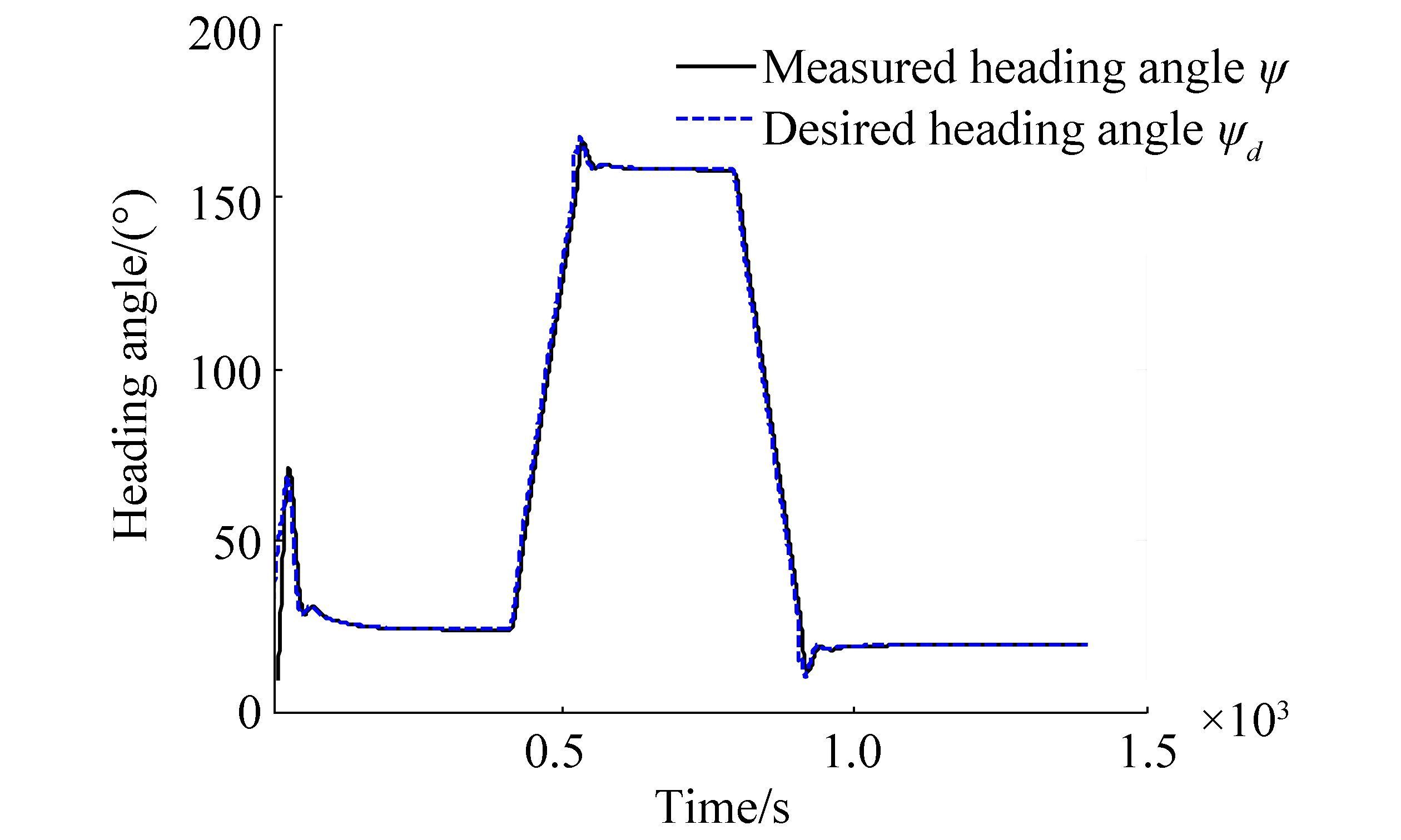
To illustrate the validity of the proposed method, parameter A will be applied in this simulation. The results of path following and heading angle tracking are depicted in Figs. 7 and 8. Fig. 7 shows the path planning with the given waypoints and the ship can follow the smooth path consisting of straight lines and circular arcs. Fig. 8 demonstrates the desired heading angle generated by the LOS guidance law and the actual ship heading angle. The sharp heading change indicates that the ship is located in the circular arc and the nearly constant heading shows that the ship is located in the straight line.
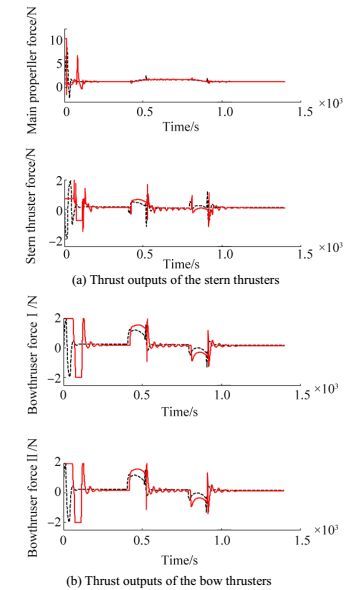
To demonstrate the advantage of including the actuators in the control closed loop, the performances with and without the inclusion of the actuator dynamics are compared in Fig. 9. By considering the actuator dynamics as a part of the maneuvering model, the thrust outputs are smoother than those defined by the controller without actuator dynamics. The proposed method can significantly reduce the wear and tear. In addition, the thrust outputs without the actuator dynamics have sharp changes which are difficult for the actuators to attain. The time lag between the control outputs and the real thrust outputs caused by the actuator dynamics tends to retard the ship's motion, and the controller without the actuator dynamics tends to compensate for it by magnifying its outputs. As the bandwidth of the actuator dynamics is close to the bandwidth of the ship's motion, the proposed method is suitable to have smoother thrust outputs since the actuator dynamics are added into the ship model.
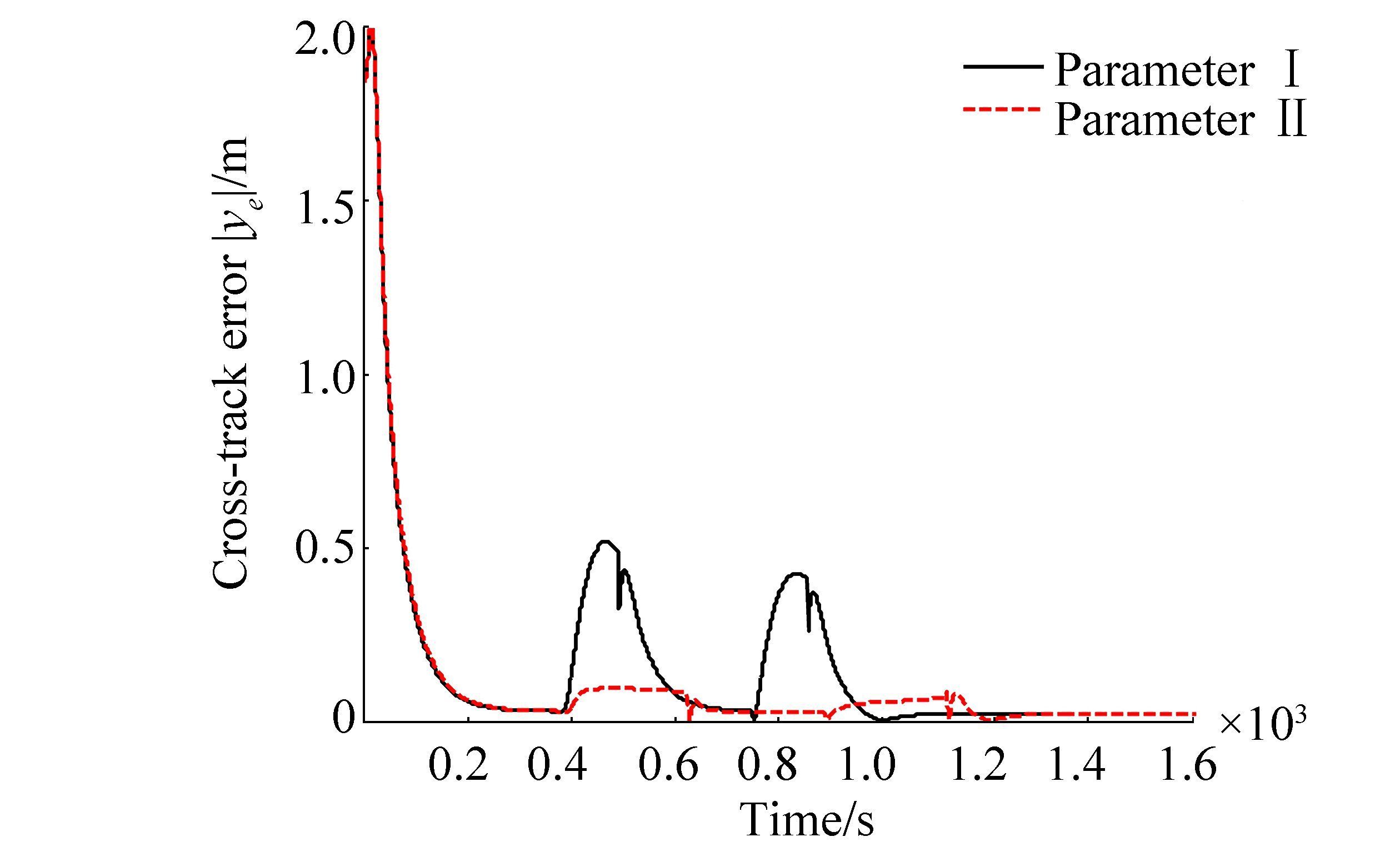
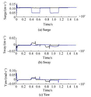
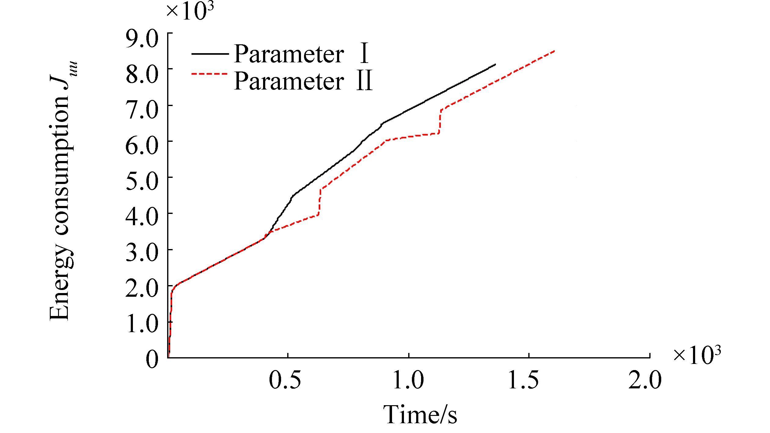
If a desired path is a curved path, then the cross-track error does not reach a steady state because it will vary as fast as the curvature of the path. Here, this paper will use the proposed method to achieve a slow-speed when the vessel is turning so that the cross-track error can be minimized. First, the deviation vector η-ηd in Section 4 should be changed from [0, 0, ψ-ψd]T to [x-xp, y-yp, ψ-ψd]T, where (xp, yp) is the origin of the PP frame shown in Section 3. The parameters set for straight lines and circles are depicted in Table 6. The comparisons of cross-track error and the speed, as well as the energy consumption with the parameters set in Table 6, are shown in Figs. 10, 11, and 12, separately. Although the ship has lower energy consumption for constant high-speed, the cross-track error is larger. As the sizes and directions of the wind, waves, and currents are assumed to be constant, the high-speed turning of the vessel will result in the big sideslip angle β and the rapid changes of the environmental forces, which will make the cross-track error larger. In addition, the ship will use more time to slow down, which will result in smaller cross-track error and larger energy consumption. The difference between parameters Ⅰ and Ⅱ is the chosen parameters for the circular arcs. To obtain a slow-speed, the desired speed can be chosen as zero and the weight of surge speed in the cost matrix Q should be reduced at the same time. The advantage of this method is that the speed when the ship is turning is more flexible because the larger weight of surge speed in the cost matrix Q will result in smaller surge speed. Thus, to obtain a different speed, one needs only to change the weight of the surge speed.
Table 6 The combined parameters Ⅰ and Ⅱ
| Parameters |
For straight lines |
For circular arcs |
| Ⅰ |
Parameter A
${\mathit{\boldsymbol{v}}_d} = {[0.1{\kern 1pt} {\kern 1pt} {\rm{m/s}},{\kern 1pt} {\kern 1pt} {\kern 1pt} 0,{\kern 1pt} {\kern 1pt} {\kern 1pt} 0]^{\rm{T}}}$ |
Parameter A
${\mathit{\boldsymbol{v}}_d} = {[0.1{\kern 1pt} {\kern 1pt} {\rm{m/s}},{\kern 1pt} {\kern 1pt} {\kern 1pt} 0,{\kern 1pt} {\kern 1pt} {\kern 1pt} 0]^{\rm{T}}}$ |
| Ⅱ |
Parameter A
${\mathit{\boldsymbol{v}}_d} = {[0.1{\kern 1pt} {\kern 1pt} {\rm{m/s}},{\kern 1pt} {\kern 1pt} {\kern 1pt} 0,{\kern 1pt} {\kern 1pt} {\kern 1pt} 0]^{\rm{T}}}$ |
Parameter D
${\mathit{\boldsymbol{v}}_d} = {[0,{\kern 1pt} {\kern 1pt} {\kern 1pt} 0,{\kern 1pt} {\kern 1pt} {\kern 1pt} 0]^{\rm{T}}}$ |
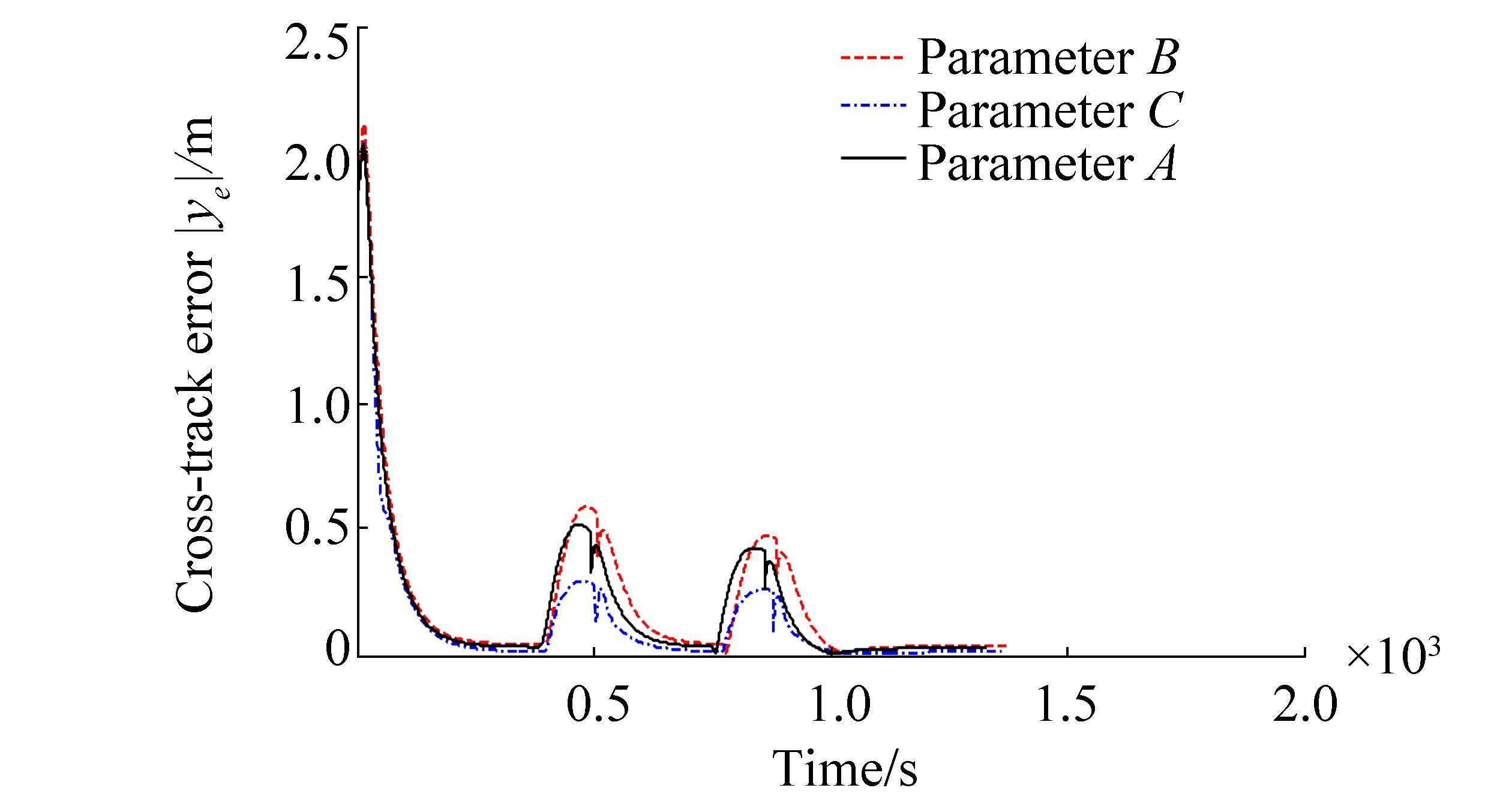
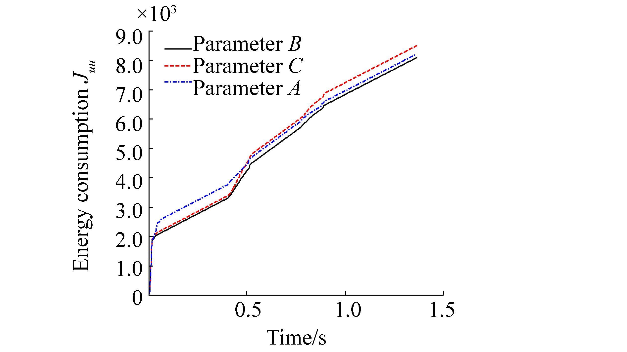
To illustrate the influences of different control parameters on energy consumption and the cross-track error, the comparisons with the set parameters in Table 5 are depicted in Figs. 13 and 14. The results clearly show that the larger weight of heading angle in the cost matrix Q will result in a smaller cross-track error, but the cost is that it will consume more energy. In addition, the smaller weight of heading angle will make the cross-track error larger and it also will consume more energy. Thus, the weight of heading angle should be chosen carefully to obtain good performance as well as less energy consumption.
7 Conclusions
A state feedback controller that is locally optimal near the origin and globally inverse optimal for the nonlinear system is derived for path following of over actuated marine crafts with actuator dynamics. To attenuate the oscillation of the control signal caused by the time lag and the slow varying environmental forces, the actuator dynamics are added into the ship model to obtain smooth thrust outputs. The proposed method can make the vessel slow down when it is turning, which can reduce the cross-track error. In addition, the cost matrices Q and R should be chosen carefully to minimize the cross-track error and the energy consumption. The stability of the closed loop system with actuator dynamics is assured through Lyapunov stability analysis.
Appendix A
The mathematical model for the realistic ship model can be given as (Fossen, 2011):
|
$\begin{array}{l}
\mathit{\boldsymbol{\dot \eta }} = \mathit{\boldsymbol{J}}(\mathit{\boldsymbol{\eta }}){\bf{ \pmb{\mathsf{ ν}} }}\\
{\mathit{\boldsymbol{M}}_{{\rm{RB}}}}\mathit{\boldsymbol{\dot v}} + {\mathit{\boldsymbol{M}}_A}{{\mathit{\boldsymbol{\dot v}}}_r} + \mathit{\boldsymbol{D}}{\mathit{\boldsymbol{v}}_r} = {\mathit{\boldsymbol{B}}_u}\mathit{\boldsymbol{u}} + {\mathit{\boldsymbol{\tau }}_{{\rm{wind}}}} + {\mathit{\boldsymbol{\tau }}_{{\rm{wave}}}}
\end{array}$
|
where MRB is the rigid-body inertial matrix and MA is the added inertial matrix. The terms, ${\mathit{\boldsymbol{\tau }}_{{\rm{wind}}}}$ and ${\mathit{\boldsymbol{\tau }}_{{\rm{wave}}}}$ are the wind and wave forces, respectively. See Fossen (2011) for detailed calculations of the wind and wave forces. The term, ${\mathit{\boldsymbol{v}}_r} \in {\Re ^{3 \times 1}}$ is the relative speed vector with respect to the effect of currents.
The relation between vr and v can be expressed as (Skjetne et al., 2004b):
|
$\begin{array}{l}
{\mathit{\boldsymbol{v}}_r} = \mathit{\boldsymbol{v}} - \mathit{\boldsymbol{J}}{(\psi )^{\rm{T}}}{\mathit{\boldsymbol{v}}_c}\\
{{\mathit{\boldsymbol{\dot v}}}_r} = \mathit{\boldsymbol{\dot v}} - r{\mathit{\boldsymbol{S}}^T}\mathit{\boldsymbol{J}}{(\psi )^{\rm{T}}}{\mathit{\boldsymbol{v}}_c}\\
{\mathit{\boldsymbol{v}}_c} = {\left[ {{V_c}\cos {\beta _c}, {V_c}\sin {\beta _c}, 0} \right]^{\rm{T}}}
\end{array}$
|
where Vc and βc are the current speed and direction in the inertial reference frame.
Appendix B
The following matrices are used in this paper:
|
$\mathit{\boldsymbol{S}} = \left[ {\begin{array}{*{20}{c}}
0 & { - 1} & 0\\
1 & 0 & 0\\
0 & 0 & 0
\end{array}} \right]\quad {\mathit{\boldsymbol{M}}_{RB}} = \left[ {\begin{array}{*{20}{c}}
{699} & 0 & 0\\
0 & {699} & { - 63.7}\\
0 & { - 63.7} & {505.03}
\end{array}} \right]$
|
|
${\mathit{\boldsymbol{M}}_A} = \left[ {\begin{array}{*{20}{c}}
{49.67} & 0 & 0\\
0 & {490.07} & {128.12}\\
0 & {128.12} & {155.36}
\end{array}} \right]\quad \mathit{\boldsymbol{D}} = \left[ {\begin{array}{*{20}{c}}
{14} & 0 & 0\\
0 & {102} & {84}\\
0 & {84} & {95}
\end{array}} \right]$
|
|
${\mathit{\boldsymbol{B}}_u} = \left[ {\begin{array}{*{20}{c}}
1 & 0 & 0 & 0\\
0 & 1 & 1 & 1\\
0 & { - 1.25} & {1.3} & {1.5}
\end{array}} \right]\quad {\mathit{\boldsymbol{T}}_u} = {\rm{diag}}(5{\kern 1pt} {\kern 1pt} {\kern 1pt} {\kern 1pt} {\kern 1pt} {\kern 1pt} {\kern 1pt} {\kern 1pt} {\kern 1pt} 5{\kern 1pt} {\kern 1pt} {\kern 1pt} {\kern 1pt} {\kern 1pt} {\kern 1pt} {\kern 1pt} {\kern 1pt} {\kern 1pt} 5{\kern 1pt} {\kern 1pt} {\kern 1pt} {\kern 1pt} {\kern 1pt} {\kern 1pt} {\kern 1pt} 5)$
|
