


 , , ,
, , ,
1 Introduction
Recent advances in sensor technology and embedded computer systems have led to developments in the field of underwater autonomy and made Autonomous Underwater Vehicles (AUVs) more viable for long-range underwater missions. However, the endurance of current AUVs is still restricted to short ranges owing to battery restrictions. The deployment of AUVs in a vast, unfamiliar, and dynamic underwater environment is a complicated process, particularly when the AUV has to promptly react to environmental changes, where real-time information is generally not known. In this context, an accurate motion-planning strategy can promote vehicle autonomy in terms of conducting different tasks in a pre-specified time interval while ensuring vehicle safety at all times. This is closely linked to vehicle autonomy in high- and low-level motion planning and its ability to prioritize the tasks that need to be completed in the limited time allowed by the battery capacity while it is concurrently guided toward its final destination in a graph-like terrain. This is ana logous to running the knapsack and the Travelling Salesman Problem (TSP) at the same time. The vehicle must effectively use the available time for a series of deployments during a long mission, which strongly depends on the optimality of the selected route between the start and destination in a waypoint-cluttered terrain. An accurate motion-planning strategy provides careful use of the AUV to achieve the mission goals and avoid the common pitfalls associated with unknown environments.
Many attempts have been made to develop single or multiple vehicle motion planning and task allocation using different strategies. Some instances of route planning system applications are in the areas of traffic control (Volf et al., 2011), real-time routing and trip planning (Ji et al., 2012), and modeling the transportation network to find the shortest paths (Geisberger, 2011). The application of a Genetic Algorithm (GA) in a dynamic route guidance system was investigated by Zou et al.(2007) . A behavior-based controller combined with a waypoint tracking scheme for AUV guidance in a large-scale underwater environment was presented by Karimanzira et al.(2014) . For energy-efficient routing ofunderwater vehicles, an artificial potential field approach was employed by Warren (1990) . An energy-efficient fuzzy-based approach using a priori known wind information in a graph-like terrain waspresented by Kladis et al.(2011) for unmanned aerial vehicle route planning. A large-scale routing and task assignment joint problem was investigated by M.Zadeh et al.(2015) . They transformed the problem space into an NP-hard graph context where in the heuristic search nature of a GA and Particle Swarm Optimization (PSO) were employed to find the best series of waypoints. Subsequently, a task-assigned route planning model based on Biogeography-Based Optimization (BBO) and PSO was introduced by M.Zadeh et al.(2016a) . This involved time-efficient routing of AUVs in a semi-dynamic operation network, where the location of some waypoints changed overtime in a bounded area.
Remarkable efforts have also been made in unmanned vehicle optimum-path planning in recent years. In general, the energy cost agrees with the path time. Real-time collision-free robot-path planning, based on a dynamic-programming shortest-path algorithm was proposed by Willms and Yang (2006) . A higher geometry maze routing algorithm was investigated by Jan et al.(2008) for optimal path planning and navigation of a mobile rectangular robot through obstacles. An A* algorithm was applied by Carroll et al.(1992) to the AUV path planning problem, taking variable vehicle speeds into account. In another research, Koay and Chitre (2013) employed an A*-based path planer to find the path with minimum energy consumption by considering ocean variations. The A* algorithm is efficient because of its heuristic search capability; however, it suffers from high computational cost in larger search spaces. Mixed integer linear programming was implemented for handling the multiple AUV path planning problems by Yilmaz et al.(2008) . A non-linear least squares optimization technique was employed by Kruger et al.(2007) for AUV path planning through the Hudson River. Path planning, based on deterministic methods, was performed by repeating a set of predefined steps that searched for the best-fit solution to the objectives Tam et al.(2009). Deterministic methods are inaccurate for large-size problems as their computational time increases exponentially with the problem size. The meta-heuristic approach, with its high computational speed, is a good alternative, particularly when dealing with NP-hard multi-objective optimization problems (M.Zadeh et al., 2016b; M.Zadeh et al., 2016c).
In most previous research (mentioned above), vehicle routing strategies have been investigated for mission planning, task allocation, and time scheduling purposes, whereas path planning strategies have been proposed to find the optimum safe path to the predefined target point. Combining these two strategies helps to overcome the shortcoming associated with each of them and achieve the objectives of both vehicle task assignment/routing and collision-free path planning by taking uncertainty and environmental dynamics into account.
To achieve successful underwater missions in a large-scale environment in the presence of a considerable amount of uncertainty, this study contributes a combinatorial framework, which comprises efficient graph route planning combined with real-time path planning, for the successful operation of a single vehicle. In this context, the graph route planner can generate the best-fit route for the available time, achieve the maximum number of highest priority tasks, and ensure that the AUV reaches its destination on time. Therefore, as a higher-level motion planner, it is in charge of the optimal distribution of tasks that are sparsely assigned to the edges of the operation network and are needed to guide the vehicle from the given starting point to the target of interest. Besides being an efficient route planner, the path generator is employed to find a conflict-free trajectory, on a smaller scale, designed to be fast enough to handle sudden changes in the environment and safely guide the vehicle through the specified waypoints with minimum time and energy costs. Constant interaction is required between the path and route planners. This is achieved by providing feedback of the conditions in the surrounding operating fields from the local path planner to the graph route planner to help decision-making during re-planning. Re-planning is performed to generate a new optimum route toward the destination, based on the last update of the decision variables. This process continues until the AUV reaches the destination. To the best of our knowledge, this combinatorial strategy is a new approach to ordinary motion planning systems because it covers the broader requirements of autonomous operations by a trade-off within the problem constraints. These constraints are time-management, mission efficiency by proper task prioritization, and safe deployment during the mission. The proposed strategy is also efficient in computational time, which enhances the system’s real-time performance.
At the core of the proposed strategy, both path and graph route planners use the BBO algorithm for satisfying their objectives. A similar hierarchical model of route-path planning, with a slight difference in the problem formulation, was also implemented by applying a PSO algorithm to both higher- and lower-level planners by M.Zadeh et al.(2016d) . It is obvious that acquiring the optimal solutions for non-deterministic polynomial-time hard problems is computationally arduous and currently, there is no polynomial-time algorithm that can solve even moderate-sized NP-hard problems. Moreover, obtaining the accurate optimal solution is only applicable to completely known environments without any uncertainty, whereas the environment modeled in this study corresponds to a highly uncertain dynamic environment. Considering the synthetic characteristic of the AUV task allocation/routing problem, whi ch generalizes both the TSP and knapsack problems, and taking into account the NP-hard complexity of the path planning problem, the BBO algorithm is applied in this research as it is one of the fastest meta-heuristic algorithms introduced for solving NP-hard problems (Zhu and Duan, 2014). The argument for using BBO to solve NP-hard problems is strong enough owing to its adaption to multidimensional spaces and proper scaling of multi-objective problems. In previous research, BBO has been shown to produce near optimum solutions w ith high probabilities. A particular characteristic of the BBO algorithm is that the solutions from one generation are transferred to the next, and the primary population does not get discarded but is modified by migration; this promotes the exploitation ability of the algorithm. This algorithm also employs a mutation operator to promote diversity in the population, which propels the individuals toward the global optima.
To examine the capability and efficiency of the proposed framework, multiple simulations were performed and implemented using MATLAB2014 by considering different dynamic uncertain environments. The organization of the study is as follows: An overview of the BBO algorithm is provided in Section 2. The formulation and implementation of the BBO-based graph route planner is demonstrated in Section 3. In Section 4, the BBO-based path planer is formulated. The evaluation criterion of the entire combinatorial model is discussed in Section 5. Discussion of the simulation results is provided in Section 6.Section 7 concludes the study.
2 Overview of the BBOBBO is an evolutionary optimization technique based on the equilibrium theory of the island bio-geographical concept (Simon, 2008). The algorithm is based on the concept of immigration, emigration, and rate of change of the number of species on an island. The geographically isolated islands are known as habitats and correspond to problem solutions. In previous research, each solution corresponds to a candidate path/route generated by the path and route planners. Each candidate solution in BBO has a quantitative performance index representing the fitness of the solution called the Habitat Suitability Index (HSI). High HSI solutions refer to islands with more suitable habitation. Habitability is related to qualitative factors known as Suitability Index Variables (SIVs), which are a vector of integers randomly initialized in advance. Each particular solution (habitat) hi has a design variable of SIV, emigration rate of μ, and immigration rate of λ. The emigration and immigration rates directly affect the population size and tend to improve the solutions. Each population solution should be evaluated before starting the optimization process. A poor solution has a higher immigration rate and a lower emigration rate. The immigration rate λ is used to probabilistically modify the SIV of a selected solution hi. Then, the emigration rates μ of the other solutions are considered, and one of them is probabilistically selected to migrate its SIV to solution hi. This process is known as migration in BBO. Subsequently, the mutation operation that tends to increase the diversity of the population and propels the individuals toward the global optima is performed. Each given solution hi is modified according to probability Ps (t), i.e., the probability of the existence of S species at time t in habitat hi. To have S species at time (t+Δt) in a specific habitat hi, one of the following conditions must hold:
1) The S species exist in hi at t, and no emigration or immigration occurs from t to (t+Δt);
2) One species immigrates onto an island already occupied by (S-1) species at t;
3) One species emigrates from an island occupied by (S+1) species at t;
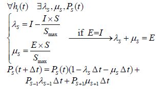
In the mathematical representation of BBO, the probability Ps (t+Δt) is the change in the number of species after time Δt, which is calculated by
|
(1) |
where λs and μs are the immigration and emigration rates when there are S species in habitat hi. I and E are the maximum immigration and emigration rates, respectively, set by the user. The maximum emigration rate occurs if all species Smax are collected in a habitat. As habitat suitability improves, its number of species and emigration rate increases and the immigration rate decreases. The probability of more than one emigration/immigration can be neglected by assuming a very small Δt. If time Δt is negligible, as Δt→0, Ps is calculated by

|
(2) |
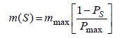
Mutation is required for a solution with low probability, whereas a solution with high probability is less likely to mutate. Hence, the mutation rate m (S) is inversely proportional to probability of the solution Ps.
|
(3) |
where mmax is the maximum mutation rate defined by the user, and Pmax is the probability of a habitat with maximum number of species Smax. BBO is applied to both the path and route planning problems. BBO is well suited to solving the vehicle path planning problem owing to the continuous nature of this problem (M.Zadeh et al., 2016b; M.Zadeh et al., 2016c; M.Zadeh et al., 2016d). Another parameter, i.e., the “keep rate, ” is initialized in advance and called an elitism parameter. This elitism parameter specifiesthe percentage of the transfer of best habitats from one generation to the next.
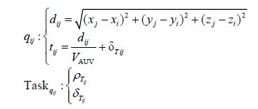
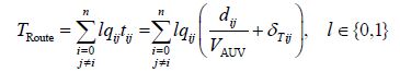
3 Formalization of BBO global route planningFor single vehicle operation, it is not possible to cover all tasks in a single mission for a large-scale operation area. Therefore, available tasks are prioritized in a way that selected edges (tasks) of the graph can guide the AUV to its destination; this is analogous to the joint discrete and syndetic space problems, which should be considered simultaneously. In this context, the proposed route planning problem can be modeled as a multi-objective optimization problem. BBO is a particular type of stochastic search algorithm representing a problem-solving technique based on biogeographical evolution, and it scales well with complex and multi-objective problems. Exploiting a priori knowledge of the underwater environment, the initial step is to transform the problem space into a graph problem. The vehicle starts its mission from the initial position WP1: (x1, y 1, z1) and should pass sufficient number of waypoints to reach the destination WPD: (xD, yD, zD). The waypoint locations are randomized according to a uniform distribution of approximately U (0, 10 000) for WPix, yand U (0, 100) for WPiz. Waypoints in the terrain are connected with an edge qi from the set of q={q1, …, qm}, where m is the number of edges in the graph. Each edge qi from the graphis assigned to a specific task from a set of Task={Task1, …, Taskk}, k∈m. Each task involves the priority parameters ρ and the absolute completion time δ, whichare randomly initialized in advance. If the route is Ri= (x1, y1, z1, …, xi, yi, zi, …, xD, yD, zD), where WPi: (xi, yi, zi) is the coordinate of any arbitrary waypoint in the geographical frame, the route travel time is calculated as follo ws:
|
(4) |
where tij is the time required to coverthe distance dij between two waypoints of WPi and WPj that includes the corresponding task’s completion time δTij and ρTij is the task priority.
The second step is to generate feasible primary routes as initial habitat populations for the BBO process. The development of a suitable coding scheme for habitat representation is the most critical step when implementing the BBO framework. Hence, efficient representation of the routes and their accurate encoding into habitats has a direct impact on the overall performance of the algorithm and optimality of the solutions. The habitat in the proposed BBO should correspond to a feasible route and include a sequence of nodes. Feasibility of a generated route is assessed using the following criteria:
· A valid route should start and end with predefined start and target nodes.
· The generated route should not include edges that are not presented in the graph.
· The multiple appearance of the same node in a route makes it invalid; this implies time wasted by repeating a task.
· The route should not traverse an edge more than once.
· The route travel time should not exceed the maximum range of AUV’s total available time.
This research conducts a priority-based strategy to generate feasible routes. To this end, a randomly initialized priority vector is assigned to a sequence of nodes. Adjacency information on the operation network and a generated priority vector are used for proper node selection along a feasible route. To prevent the generation of infeasible routes, some modifications are applied. To generate a feasible route in a graph based on topological information, each node takes positive or negative priority values in the specified range [-100, 100]. Adjacency relations are used to add nodes to a specific route in sequence, one-by-one, according to the priority vector and adjacency matrix. The first node is selected and added to the sequence as the start node. Then, from the adjacency matrix, the nodes connected to node-1 are considered. The node with the highest priority in this sequence is selected and added to the route sequence as the next visited node. Aselected node in the route sequence obtains a large negative priority value that prevents repeated visits to it. Then, the visited edges get eliminated from the adjacency matrix so that the selected edge will not be a candidate for future selection. This reduces memory usage and time complexity for large and complex graphs. This procedure continues until a legitimate route is built (destination visited). To satisfy the termination criteria of a feasibl e route, if the route ends with a non-destination node and/or the length of the route exceeds the number of existing nodes in the graph, the last node of the sequence will be replaced by the index of the destination node. The process of BBO-based global route planning is summarized in the flowchart in Fig. 1.

|
| Figure 1 Process of the BBO-based global route planning |
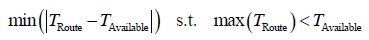
When a number of feasible routes have been generated and the habitat population initialized, the optimization process starts to find the optimum global route through the given waypoints according to the flowchart in Fig. 1. The goal is to find a route that achieves the maximum number of highest priority tasks in the time allowed by the battery capacity. The problem involves multiple objectives that should be satisfied during the optimization proces s. In this regard, the objective function of the route planner is defined as a form of hybrid cost function comprising weighted functions that need to be maximized or minimized. The total route cost function is formulated in Section 5. In this model, the route travel time should approach the mission available time, thereby maximizing the use of the available time.
|
(5) |
|
(6) |
where TRoute is the time required to complete the route, TAvailable the total mission time, and l the selection variable.
4 Formalization of BBO local path planningThe local path planner operates in the context of the global route planner and concurrently generates a safe collision-free path between pairs of waypoints while encountering the dynamicity of the environment. In this section, the conceptual and mathematical representation of the local path planning framework is presented. Path planning is an optimization problem where in the main objective is to find a time-optimum collision-free local path ℘i (shortest path) between a specific pair of waypoints in the presence of different types of uncertain obstacles. The resultant path should be safe and flyable (feasible). The dynamicity of the operational environment Γ3D addresses encountering different types of static and floating obstacles Θ with uncertain positions and velocities, where the floating obstacles are affected by current flow.
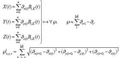
The proposed path planner in this study, generates potential trajectories ℘i:{℘1, ℘2, …} using B-Spline curves captured from a set of control points, θ={θ1, θ2, …, θi, …, θn}, in a problem space with coordinates of θ1: (x1, y1, z1), …, θn: (xn, yn, zn), where n is the number of corresponding control points. These control points play a significant role in determining the optimal path. The mathematical description of the B-Spline coordinates is given by (7) :
|
(7) |
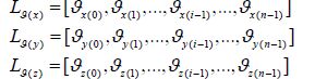
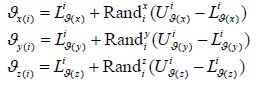
where the X (t), Y (t), and Z (t) are the vehicle’s positions along the path at time t, the Bi, K (t) is the curve blending functions, and K is the order of the curve representing its smoothness, where larger values of K correspond to smoother curves. For further information, refer to Nikolos et al.(2003) . All control points should be located in respective search regions constrained to the predefined bounds of βiθ=[Uθi, Lθi]. If θi:[x (i), y (i), z (i) ] represents one control point in Cartesian coordinates; the lower bound Lθi; and the upper bound Uθi of all control points at (x-y-z) coordinates is calculated by (8), (9), respectively. Then, each control point θi can be generated from (10) :
|
(8) |

|
(9) |
|
(10) |
In the proposed BBO-based path planning problem, each habitat hi corresponds to the coordinates of the B-Spline control points {θ1, …, θn} used in path generation. Each habitat hi has an HSI and is represented by a real vector of n-dimension, which is randomly initialized randomly in advance. A habitat is a vector of n, SIVs (hi:{ χ1, χ2, …, χn}), generated randomly and defined as a parameter to be optimized.
The migration and mutation operations are then performed to lead the habitats toward the optimal solution. As the BBO algorithm iterates, each habitat gets attracted toward its respective best position based on its SIV. The pseudo-code of the BBO algorithm and its mechanism in the path planning process is provided in Fig. 2.

|
| Figure 2 BBO path planning pseudo code |
The path planner is applied to a small-scale area, and the AUV is considered to have constant thrust power, therefore, the battery usage for a path is a constant function of the time and distance traveled. Performance of the generated path is evaluated based on the overall collision avoidance capability and time consumption, which is proportional to the energy consumption and distance traveled. Fig. 3 shows a schematic of the AUV path planning process.

|
| Figure 3 Operational diagram of the AUV path planning process |
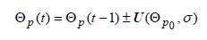
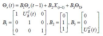
In terms of collision avoidance, an obstacle’s velocity vectors and coordinates can be measured by sonar sensors and uncertainty modeled by a Gaussian distribution. The state of obstacle (s) is continuously measured and sent to a state estimator, which provides an estimation of the future states of the obstacles for the local path planner. The state predictor estimates the obstacles’ behavior during vehicle deployment within a specified operation window. To evaluate the performance of the proposed path planner, four different types of obstacles are considered in this study; each obstacle is represented by three components: position, radius, and uncertainty Θ (i) : (Θp, Θr, , ΘUr). The first type is a static known obstacle; its location is known and can be obtained from an offline map. No uncertainty growth is considered for positions of this type. The second type, classified as quasi-static obstacles, is usually known as no-fly zone. The obstacles in this category have an uncertain radius, which varies withina specified boundary and has a distribution of approximately (Θp, σ0), where the value of Θr in each iteration is independent of its previous value. A self-motivated moving obstacle is the third type. This has a motivated velocity that shifts it from position A to B. Therefore, its position shifts in a random direction with an uncertainty rate that is proportional to time, see (11). The last type is a moving obstacle that is affected by current forces and also has self-motivated velocity in a random direction, see (11) and (12). Here the effect of the current is represented by uncertainty propagation proportional to the current magnitude URC=|VC|~ (0, 0.3), which radiates from the center of the obstacle in a circular format, see Fig. 4.

|
| Figure 4 Graphical representation of uncertain floating/moving obstacles |
|
(11) |
|
(12) |
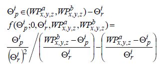
where ΘUrσ is the rate of change of the object’s position, and X (t-1) ~N(Θp, σ0) is the Gaussian normal distribution assigned to each obstacle, which gets updated at each iteration t. In all cases, obstacle position Θp is initialized using a normal distribution of approximately (0, σ2) bounded by the position of the start and target waypoints WPx, y, za<Θp<WPx, y, zb. Therefore the obstacle’s position Θp has a truncated normal distribution, and its probability density function is defined as:
|
(13) |
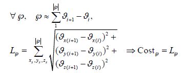
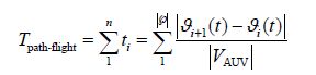
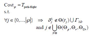
The obstacle radius is initialized using a Gaussian normal distribution of approximately (0, 100) . This operating zone shifts to the next pair of waypoints in a sequence provided by the graph route planner. To evaluate the path ℘i, the path cost function is defined on the basis of the time required to travel along the path between two waypoints (Tpath-flight).
|
(14) |
|
(15) |
|
(16) |
where j is any arbitrary point on the generated path and Cost℘is the path cost function. The corresponding generated path should not cross the forbidden area covered by the obstacle Θ (NΘ) : (Θp, Θr, , ΘUr), where NΘ is the number of obstacles. The generated path gets penalty value for colliding any obstacle. The generated path gets penalty values for colliding with any obstacle. In general, this process promotes the algorithm’s evolution toward generating a feasible solution.
5 Evaluation of the combined BBO motion planning modelAs mentioned earlier, the local path planner operates in the context of the global route planner and concurrently generates a safe collision-free path between pairs of waypoints while encountering the dynamicity of the environment. After passing each waypoint, the path absolute time Tpath-flight is calculated. This generated path time Tpath-flight is then compared to the expected time TExpected for completing the distance between a specified pair of waypoints. If Tpath-flight becomes smalle r than TExpected, it means that no unexpected difficulties were encounteredand the vehicle can continue along the provided route. However, if Tpath-flight exceeds TExpected, this means that the AUV has faced a challenge during its deployment. It is obvious that a certain amount of the mission available time TAvaliable is wasted in coping with thesedifficulties; therefore, the previously defined route is no longer the optimum route. In this situation, it is essential to re-plan a new optimum route according to the mission updates. Hence, the third problem is focused on route re-planning based on environmental changes and time updates during vehicle deployment. The re-planning process is clarified in Fig. 5.

|
| Figure 5 Requisition for the re-planning process |
Another issue is the computational burden of the re-planning process. After encountering an unexpected event, if the previously found optimum route is ignored, the global route planner is recalled to find a new optimum route from the predefined start point to the destination. The re-planning scheme does not guarantee at least a quasi-real-time solution as it includes considerable computational burden. For significantly reducing the computational burden involved in re-planning, when re-routing is required in any situation, based on TAvaliable updates, the passed edges are eliminated from the operation network (so the search space shrinks); the location of the present waypoint is then considered as the new starting position for both the local and global motion planners. The global route planner then tends to find the optimum route based on new information and updated network topology. For example, in Fig. 6 the initial optimum route is a sequence of waypoints {1-2-5-7-12-15-13- 16-11-17-D}; and after re-planning, this is replaced by a new sequence of {15-18-16-D}. During deployment between two waypoints, the local path planner can incorporate dynamic changes in the environment. This process continues until the mission ends and the vehicle reaches the required destination point. The trade-off between the available mission time and mission objectives is a critical issue that can be adapted and performedby the route planner. This should be fast enough to track environmental changes and promptly re-plan a new route fitted to the updated available time. A schematic representation of the combinatorial strategy is given in Fig. 7.

|
| Figure 6 Graphical representation of the operating area covered by waypoints, and local/global motion planning and re-planning processes |

|
| Figure 7 Proposed combinatorial strategy for dynamic guidance of an AUV |
The route cost has a direct relation with the distance between each pair of selected waypoints with respect to Eqs.(4) - (6). Hence, the path cost Cost℘for any optimum local path is used in the context of the graph route planner. The model seeks an optimal solution from the best combination of path, route, and task cost. After visiting each waypoint, the re-planning criteria are investigated. Computation cost is encountered each time that re-planning is required. Thus, the total cost for the model is defined as

|
(17) |
where δTij and ρTij represent the completion time and priority value of the task assigned to qij, respectively. The computational time Tcompute is spent for checking the re-planning criteria. r is the number of repeats in the re-planning procedure. The path cost of Cost℘, task completion time and Tcompute are utilized in calculation of the CostRoute.
6 Discussion of simulation resultsIn this section, simulation results from the performance evaluation of the proposed framework are demonstrated. The main purpose of the simulation is to analyze the performance of each motion planner and the functionality of the entire framework in terms of increasing mission productivity (task assignment and time management) along with ensuring vehicle safety during the mission. To verify the efficiency of the proposed strategy, first, the efficiency of the local path planner is individually assessed. Second, the performance of the global route planner is investigated. Finally, the overall coherence of the framework in terms of mission timing and accurate co-operation of global and local planners is investigated and evaluated. In this study, the optimization problem was performed on a desktop PC with an Intel i7 3.40 GHz quad-core processor using MATLAB®R2014a.
6.1 Evaluation of the path plannerIt is assumed that the AUV travels at aconstant velocity VAUV between two waypoints. The ocean environment is modeled as a three-dimensional environment Γ3Dcomprising known static, uncertain static, and floating/ moving obstacles. In the path planning simulation, obstacles are generated randomly from different categories and configured individual ly on the basis of the given relations in Section 2. These assumptions play an important role in efficient path planning and coping with dynamic environmental changes. The path planner generates the potential AUV trajectories using B-Spline curves captured from a set of control points. The fitness of the generated path is evaluated using Eq.(16). Three different scenarios are implemented in the simulation to assess the accuracy of the proposed local path planner. In the first scenario, the AUV starts its deployment in a pure static operating field containing static known and static uncertain obstacles, where the vehicle is required totravel the shortest collision-free distance to reach the specified target waypoint. Making the AUV’s mission more challenging, in the second scenario, the robustness of the method is tested in a dynamic environment, which includesmoving obstacles with self-motivated velocities in a random direction. In the third scenario, the mission is complicated more by adding the impact of current forces using floating obstacles with uncertain positions. The purpose of increasing the obstacle complexity is to evaluate the sustainability of the path planner’s performance when dealing with increasingly complex environments and evaluating the ability of the method to balance searching unexplored operating fields and safely moving toward the target waypoint. For this purpose, a distinctnumber of runs are performed to assess if the performance of the method satisfies the problem constraints for all three scenarios. The BBO configuration for all scenarios was set as follows: the habitat population (nPop) and maximum number of iterations (Itermax) were set at 50 and 100, respectively. The number of kept and new habitats was set at 10 and 40, respectively. The emigration rate is generated by μ=linspace (1, 0, nPop), and the immigration rate defined as λ=1-μ. The maximum mutation rate is set at 0.1. The number of control points for each B-Spline path is set at 8. The accuracy of the algorithm is tested for all scenarios and presented in Figs. 8-10 for different number of obstacles. The path should be re-generated simultaneously to avoid crossing the corresponding collision boundaries; this process is repeated until the vehicle reaches the target waypoint.

|
| Figure 8 Performance of the path planner in the first scenario |

|
| Figure 9 Simulation results associated with the second scenario |

|
| Figure 10 Performance of the path planner in the third scenario |
Fig. 8 illustrates the performance of the path planner in the first scenario, where a random number of static obstacles, with growing radii, occur in the proposed operating field. The simulation results of the second scenario are demonstrated in Fig. 9. In Fig. 9 (a) , the generated path exposed to moving obstacles is shown. The obstacles’ movement is simulated in accordance with a pre-specified rate of uncertainty based on time. Considering the third scenario, the uncertainty around the obstacles in Fig. 10 (a) propagates from the center of the object with a growth rate proportional to current velocity |VC|~N (0, 0.3) in all directions. In addition, the obstacles move with a self-motivated velocity in a random direction. Gradual increments of the collision boundary of each obstacle are presented in Fig. 10 (a) . This figure shows that the local path planner can generate a collision-free path, eve n in a dynamic operating field, with an acceptable rate of convergence for adefined optimality metric such as flight time, as shown in Fig. 10 (b) . The variations, in terms of cost and violation functions per iteration, are more significant when they are compared with the first and second scenarios; however, the algorithm still experiences a moderate convergence that guarantees feasible and optimal solutions.
As inferred from Figs. 8 (c) and (d), 9 (c) and (d), and 10 (c) and (d) , the algorithm accurately tends to minimize path travel time and cost over 100 iterations, while its performance is almost stable in the increasing complex environments. Also note worthy, from analysis of the results we find that the cost variation range in all scenarios decreases in each iteration, which means that the algorithm accurately converges to the optimum solution with minimum cost. Tracking the variation in the mean cost and mean violation, represented by red crosses in the middle of the error bar graphs, shows that the algorithm forces solutions to the optimum answer (path) with minimum cost, and efficiently manages the path, eliminating the collision penalties, within 100 iterations.
In summary, it is obvious that in all three scenarios the algorithm provides solutions that satisfy the collision constraints for all types of obstacle; it tends to minimize the path travel time as this is the main optimization factor for the path planner.
Additional to the common performance criterion investigated above, two more performance factors are highlighted for the purpose of this research and are discussed along with the evaluation of the entire model. The first highlighted index is the path planner’s computational time, because it must synchronize to the global route planner and operate concurrently. Hence, large computational time causes a delay in the local path planner andgraph route planner synchronization, which causes interruption in the routine process of the whole system.
6.2 Evaluation of the global route plannerA number of performance metrics have been investigated to evaluate the optimality of the proposed solutions by the route planner in different network topologies, such as the number of completed tasks, total obtained weight, total cost, and time optimality of the generated route. Reliability percentage of the route is another metric representing the chance of the mission success; it is defined based on route violation, which is a weighted function of travel time and feasibility of the route. The BBO, in this circumstance, is configured with a habitat population size of 150, 300 iterations, habitat keep rate of 0.6, emigration rate of μ=0.2 immigration rate of λ=1-μ, and maximum mutation rate set at 0.8. Habitat keep rate is the ratio of the best solutions selected to be transferred to the next generation (as mentioned in the pseudo-code in Fig. 2). The performance of the algorithm is tested on graphs with diverse topologies including graphs with 20, 50, 80, and 100 nodes. Table 1 demonstrates the impact of graph complexity on the functionality of the route planner.
| Performance metrics | Graph complexity-nodes | Graph complexity-edges | CPU run time | Best cost | Total mission time/s | Route travel time/s | Total distance | Total weight | N-Tasks | Violation |
| Solution 1 | 20 | 202 | 12.558 | 0.041 3 | 21 200 | 20 848 | 62 543 | 40 | 15 | 0.0 |
| Solution 2 | 50 | 1197 | 16.177 | 0.023 1 | 32 400 | 30 062 | 90 187 | 55 | 19 | 0.0 |
| Solution 3 | 80 | 3099 | 22.432 | 0.019 6 | 39 600 | 34 686 | 104 059 | 63 | 23 | 0.0 |
| Solution 4 | 100 | 4886 | 27.487 | 0.017 1 | 45 360 | 45 387 | 136 161 | 78 | 27 | 0.008 |
The violation index has a positive value when the route time exceeds the available time. Violating the cost function causes the algorithm to generate feasible solutions. It is noted from the simulation results in Table 1 that the violation value for all four examined complexities is almost zero, which means that the generated routes accurately respect the defined time constraint. On the other hand, the optimum route corresponds to the route with the travel time closest to the total mission time, meaning that the AUV makes maximum use of the total available time. As depicted in Table 1, in all four cases the route travel time approached the value of the total mission time but did not exceed it, which confirms the efficiency of the route planner in satisfying the objectives and constraints.
Considering the influence of the graph topology on the presented solutions in Fig. 11, the run time increases linearly as the number of nodes in the graph increases; however, in all cases, it remains within the bounds of a stable real-time solution. From the cost variations in Fig. 12, it is obvious that the performance of the proposed route planner is stable with an increasing search space size; again a major challenge for deterministic strategies, which makes them inappropriate for real-time applications.

|
| Figure 11 Computational time variation vs. graph complexity |

|
| Figure 12 Cost variation of the BBO-based route planning for different graph complexities in 300 iterations |
The proposed combinatorial framework aims to makemaximum use of the mission available time to increase the number of completed higher-priority tasks in a single mission, while guaranteeing on-time mission termination and vehicle safe deployment. Accurate synchronization of the inputs and outputs of the engaged path/route planners and their concurrent cooperation are the most important requirements for the stability of the model regarding the main objectives above. To this end, the robustness of the model was evaluated by the simulation of 10 underwater missions in 10 individual experiments, with initial conditions that closely matched actual underwater mission scenarios. The initial configuration of the operation network was set to 40 waypoints and 1 320 edges, involving a fixed sequence of tasks with specified characteristics (priority and completion time) in a 10 km2 (x-y), 100 m (z) space. The waypoint locations were initialized using a uniform distribution of ~U (0, 10 000) for WPix, y and approximately U (0, 100) for WPiz. The mission available time for all experiments was fixed at TAvailable=10 800 s, equal to 3 h. The vehicle starts its mission at initial location WP1 and ends at WP40. As mentioned earlier, it is assumed that the vehicle moves with a constant (3 m/s) velocity. To examine the performance and stability of the proposed architecture, the operating field was modeled as a realistic underwater environment. In Tables 2 (a), (b) the process of the combinatorial strategy at different stages of a specific mission scenario is shown.
| (a) Global-route | ||||||||||
| Call No. | Start | Target | Task No. | Weight | Route cost | TCPU | TAvailable | TRoute | Validity | Route sequence |
| 1 | 1 | 40 | 8 | 38 | 0.430 | 23.1 | 10 800 | 10 460 | Yes | 1-24-7-25-32-11-26-34-40 |
| 2 | 25 | 40 | 6 | 27 | 0.320 | 20.9 | 5 862.8 | 5 831 | Yes | 25-36-26-27-33-5-40 |
| 3 | 33 | 40 | 1 | 14 | 0.610 | 19.8 | 1 757.6 | 1 728 | Yes | 33-40 |
| (b) Local-path | ||||||||||
| Route ID | PP call No. | Edges | Violation | Path cost | TCPU | Tpath-flight | TExpected | TAvailable | Replan flag | PP flag |
| Route-1 | 1 | 1-24 | 0.000 000 | 0.450 | 41.6 | 1 532.7 | 1 666.7 | 9 267.3 | 0 | 1 |
| 2 | 24-7 | 0.000 000 | 0.510 | 40.3 | 1 702.3 | 1 872.7 | 7 565 | 0 | 1 | |
| 3 | 7-25 | 0.000 000 | 0.460 | 36.4 | 1 702.1 | 1 673.1 | 5 862.8 | 1 | 0 | |
| Route-2 | 1 | 25-36 | 0.000 031 | 0.115 | 37.8 | 467.2 | 535.3 | 5 395.6 | 0 | 1 |
| 2 | 36-26 | 0.000 000 | 0.311 | 43.7 | 1 153.2 | 1 210 | 4 242.4 | 0 | 1 | |
| 3 | 26-27 | 0.000 000 | 0.369 | 39.1 | 1 306.2 | 1 333.4 | 2 936.3 | 0 | 1 | |
| 4 | 27-33 | 0.000 007 | 0.232 | 39.7 | 1 178.7 | 1 068.3 | 1 757.6 | 1 | 0 | |
| Route-3 | 1 | 33-40 | 0.000 000 | 0.511 | 40.6 | 1 705.4 | 1 727.7 | 52.1 | 0 | 0 |
The mission starts by calling the global route planner for the first time; a valid optimum route is then generated to makemaximum use of the available time (valid route TRoute≤TAvailable). Referring to Table 2, the initial optimum route consists of 8 tasks with total weight of 38, cost of 0.430 and estimated completion time of TRoute=10 460 s. In the second phase, the local Path Planner (PP) is recalled to generate the optimum collision-free path through the listed sequence of waypoints included in the initial route. Referring to Table 2 (b) , the local path planner adopts the first pair of waypoints {1-24} and generates the optimum path between locations WP1 and WP24 with total cost of the 0.450 and travel time of Tpath-flight=1 532.7 s, which is smaller than expected travel time TExpected=1 666.7 s. The TExpecte d for the local path planner is calculated based on the estimated travel time for the generated route (TRoute). If Tpath-flightis smaller than TExpected, the re-planning flag is zero and the initial optimum route is still valid and optimum- so the vehicle is therefore allowed to travel to the next pair of waypoints included in initial optimum route.
After each run of the path planner, the path time Tpath-flight is subtracted from the total available time TAvailable. The second pair of waypoints {24-7} is shifted to the path planner and process is repeated. However, if Tpath-flight exceeds TExpected, (occurred in {7-25}), the re-planning flag becomes 1, which means that some of the available time is wasted passing between WP7 and WP25 due to collision avoidance. In such a case, TAvailable also gets updated and the visited edges (1-24, and 24-7) get eliminated from the graph. After this, the global route planner is recalled to generate a new optimum route, based on the updated operation network and TAvailable from the current waypoint WP25 to the predefined destination WP40. In the simulation results presented in Table 2, the global route planner is recalled 3 times and the local path planner is called 8 times within 3 optimum routes. This interplay between the modules continues until vehicle reaches the destination (success) or TAvailable gets a minus value (failure: vehicle runs out of battery). In this case, the final route is the sequence of waypoints including {1-24-7-25-36-26-27-33-40} with a total cost of 1.128, total weight of 31, and total time of 10748.8 s.
The most appropriate outcome for a mission is completion of the mission with minimum remaining time, which means that the mission available time has been maximized. Referring to Table 2 (b) , the remaining time is 52.1 s, and compared to mission available time of TAvailable=10 800 s, is remarkably close to zero. Therefore, the architecture’s performance can be represented by mission time (or remaining time). It is noteworthy tha t ensuring the on-time termination of the mission is a priority for the proposed model, rather than maximizing the completed tasks in a single mission. This is a big concern for vehicle safety and a large penalty value is assigned to the global route planner to strictly prevent it generating routes with TRoute greater than TAvailable. The time-management performance of the model over 10 experiments is shown in Figs. 13 and 14.
The main purpose is to show that the collision and time violation of the whole system is controlled, which means safe deployment is guaranteed, and, more importantly, ensures on-time termination of the mission. As apparent from Fig. 13 (a) , the proposed model is capable of making maximum use of mission available time, as apparently the mission time in all experiments approached TAvailable. It is important to mention that all generated solutions meet the constraints, denoted by an upper bound of 10 800 s; this confirms the stability of the proposed strategy for any arbitrary mission in terms of time management and satisfying the mission objectives. Moreover, all missions were completed with a low computation burden as indicated by the CPU time index in Fig. 13 (b) . Noteworthy from analysis of the simulation results in Table 2, is that both planners take a very short CPU time for all experiments, which makes the model highly accurate for real-time application. It is evident from Fig. 13 (b) that the variation in CPU time for the model is within a similar range for all experiments, which proves the inherent stability of the model. In addition, the model’s cost variation is show in Fig. 14 for each motion planner in all 10 experiments. It is clear that the cost variation in the local and route planners (in multiple recall) for all experiments lie within a similar range, and are centralized over the mean solution cost, which that confirms the stability of the model’s performance.

|
| Figure 13 Performance of the combinatorial model in maximizing mission performance by maximizing the mission time constrained to available time threshold, and total CPU time for 10 different experiments |

|
| Figure 14 Model stability for motion planners cost variation over 10 experiments |
The path planner gets a violation if any collision occurs. On the other hand, the global route planner gets a penalty (violation) when the route time exceeds the available time. It is clear from Fig. 15 that both global route and local path planners accurately manage the total system violation from multiple recalls over the 10 missions, as the variation in the violation value for both planners is almost equal to zero, which is negligible.

|
| Figure 15 Model stability for controlling total violation in multiple experiments |
Tables 3shows the performance and stability of the model in terms of mission productivity, by the quantitative measurement of two significant mission metrics, i.e., number of completed tasks, and total captured weight over 10 missions. Analysis of the results in Figs. 13-15 and Table 3 show the functionality and stability of the model when dealing with problem space deformation and confirms its real-time capability.
| Mission No. | Task No. | Total weight | Total cost | Total TCPU |
| 1 | 8 | 31 | 1.128 | 428.1 |
| 2 | 10 | 31 | 1.073 | 681.2 |
| 3 | 6 | 25 | 1.402 | 427.2 |
| 4 | 8 | 29 | 1.327 | 702.8 |
| 5 | 7 | 33 | 1.283 | 385.0 |
| 6 | 9 | 30 | 1.212 | 557.9 |
| 7 | 7 | 36 | 0.923 | 306.2 |
| 8 | 8 | 28 | 1.330 | 741.2 |
| 9 | 9 | 27 | 1.414 | 527.7 |
| 10 | 8 | 28 | 1.306 | 575.2 |
In this research, a new deliberative framework was developed to raise the potential for AUVs to have a certain degree of autonomy, i.e., to trade-off between completion, time management, and robust motion planning to successfully complete a mission. At the top level of the framework, a graph route planner promotes vehicle autonomy in terms of time management and task assignment in a graph-like terrain, where each edge of the graph is assigned to a task. Accordingly, at the lower level, the path planner tends to find the shortest collision-free trajectory between each pair of listed waypoints along a generated global route.
This approach can efficiently respond to environmental changes and is executable for real-time implementation. Based on various simulations, the stability and performance of the framework is verified. It is clear from the results that the presented model is efficient and accurate in producing real-time near optimal solutions, in which the efficiency of the model is relatively independent of both size and complexity of the operating field.
Future work will comprise a more extensive version of the proposed architecture, using actual sensory information and keeping one step ahead of environmental change, as this is useful in reality. In addition, experimental validation of the framework will be performed on a real vehicle.
| Carroll KP, McClaran SR, Nelson EL, Barnett DM, Friesen DK, Williams GN, 1992. AUV path planning: an A* approach to path planning with consideration of variable vehicle speeds and multiple, overlapping, time-dependent exclusion zones. IEEE Conference of Autonomous Underwater Vehicle Technology. DOI: 10.1109/AUV.1992.225191 |
| Geisberger R, 2011. Advanced route planning in transportation networks. PhD thesis, Karlsruhe Institute of Technology, Karlsruhe, 1-227. |
| Jan GE, Chang KY, Parberry I, 2008. Optimal path planning for mobile robot navigation. IEEE/ASME Transactions on Mechatronics, 13(4), 451–460. DOI:10.1109/TMECH.2008.2000822 |
| Ji M, Yu X, Yong Y, Nan X, Yu W, 2012. Collision-avoiding aware routing based on real-time hybrid traffic information. Journal of Advanced Materials Research, 396-398, 2511-2514. |
| Karimanzira D, Jacobi M, Pfuetzenreuter T, Rauschenbach T, Eichhorn M, Taubert R, Ament C, 2014. First testing of an AUV mission planning and guidance system for water quality monitoring and fish behavior observation in net cage fish farming. Information Processing in Agriculture, 1(2), 131–140. DOI:10.1016/j.inpa.2014.12.001 |
| Koay TB, Chitre M, 2013. Energy-efficient path planning for fully propelled AUVs in congested coastal waters. IEEE OCEANS'13 Bergen, Bergen. DOI: 10.1109/OCEANS-Bergen.2013.6608168 |
| Kladis GP, Economou JT, Knowles K, Lauber J, Guerra TM, 2011. Energy conservation based fuzzy tracking for unmanned aerial vehicle missions under a priori known wind information. Engineering Applications of Artificial Intelligence, 24(2), 278–294. DOI:10.1016/j.engappai.2010.10.013 |
| Kruger D, Stolkin R, Blum A, Briganti J, 2007. Optimal AUV path planning for extended missions in complex, fast flowing estuarine environments. IEEE International Conference on Robotics and Automation, Roma. DOI: 10.1109/ROBOT.2007.364135 |
| M.Zadeh S, Powers D, Sammut K, Lammas A, Yazdani AM, 2015. Optimal route planning with prioritized task scheduling for AUV missions. IEEE International Symposium on Robotics and Intelligent Sensors, Langkawi, 7. |
| M.Zadeh S, Powers D, Yazdani AM, 2016a. A novel efficient task-assign route planning method for AUV guidance in a dynamic cluttered environment. IEEE Congress on Evolutionary Computation (CEC), Vancouver. |
| M.Zadeh S, Powers MWD, Sammut K, Yazdani AM, 2016b. Differential evolution for efficient AUV path planning in time variant uncertain underwater environment. arXiv:1604.02523 |
| M.Zadeh S, Yazdani A, Sammut K, Powers DMW, 2016c. AUV rendezvous online path planning in a highly cluttered undersea environment using evolutionary algorithms. robotics (cs.RO). arXiv:1604.07002 |
| M.Zadeh S, Powers DMW, Sammut K, Yazdani A, 2016d. Toward efficient task assignment and motion planning for large scale underwater mission. Robotics (cs.RO).arXiv:1604.04854 |
| Nikolos IK, Valavanis KP, Tsourveloudis NC, Kostaras AN, 2003. Evolutionary algorithm based offline/online path planner for UAV navigation. IEEE Trans. Syst. Man, Cybern. B, Cybern. 33(6), 898-912. DOI: 10.1109/tsmcb.2002.804370 |
| Simon D, 2008. Biogeography-based optimization. IEEE Transaction on Evolutionary Computation, 12, 702–713. DOI:10.1109/TEVC.2008.919004 |
| Tam C, Bucknall R, Greig A, 2009. Review of collision avoidance and path planning methods for ships in close range encounters. Journal of Navigation, 62(3), 455–476. DOI:10.1017/S0373463308005134 |
| Volf P, Sislak D, Pechoucek M, 2011. Large-scale high-fidelity agent based simulation in air traffic domain. Cybernetics and Systems, 42(7), 502–525. DOI:10.1080/01969722.2011.610270 |
| Warren CW, 1990. Technique for autonomous underwater vehicle route planning. IEEE Journal of Oceanic Engineering, 15(3), 199–204. DOI:10.1109/48.107148 |
| Willms AR, Yang SX, 2006. An efficient dynamic system for real-time robot-path planning. IEEE Transactions on Systems, Man, and Cybernetics, Part B: Cybernetics, 36(4), 755–766. DOI:10.1109/TSMCB.2005.862724 |
| Yilmaz NK, Evangelinos C, Lermusiaux PFJ, Patrikalakis NM, 2008. Path planning of autonomous underwater vehicles for adaptive sampling using mixed integer linear programming. IEEE Journal of Oceanic Engineering, 33(4), 522–537. DOI:10.1109/JOE.2008.2002105 |
| Zhu W, Duan H, 2014. Chaotic predator–prey biogeography-based optimization approach for UCAV path planning. Journal of Aerospace Science and Technology, 32(1), 153–161. DOI:10.1016/j.ast.2013.11.003 |
| Zou L, Xu J, Zhu L, 2007. Application of genetic algorithm in dynamic route guidance system. Journal of Transportation Systems Engineering and Information Technology, 7(3), 45–48. DOI:10.1016/S1570-6672(07)60021-X |