


 , ,
, ,
1 Introduction 1.1 Background
The rise in energy demand has increased the offshore oil and gas production dramatically in the last two decades. The new trend of replacing coal with natural gas in the power sector partially influenced the natural gas production in the world. To cater to this ever increasing natural gas demand, oil and gas producers are exploring more offshore natural gas resources. In the Arctic the largest portion of the offshore resources is found to be natural gas (85% is natural gas against 13% oil - Ferentinos, 2013). 85% of Brazil’s natural gas reserves are known to be located offshore (U.S.EIA, 2014). With the growth of offshore gas production, the tendency is to produce more gas from deepwater than the shallow water. Permits issued for US Gulf of Mexico in 2012 were nearly 100 for deepwater (well) drilling, while only 50 were for shallow water drilling (Ferentinos, 2013). The increase of natural gas production has increased the risk of an accidental underwater gas releases. Deep Water Horizon (DWH) accident in the Gulf of Mexico in 2010 is an example for such a major oil and gas release. In such incidents computer models play an important role in predicting the fate and transport of gas and surfacing rates, for contingency planning and emergency response. After the DWH incident there appears to be a tendency in the energy industry to use models more frequently for risk assessment and contingency planning. Many computer models have been developed to simulate underwater oil and gas releases, while only a few models have the capability to simulate the fate of deepwater gas releases (e.g. Johansen, 2000; Zheng et al., 2003; Yapa et al., 2010).
The available models have shown an acceptable level of performance in predicting the spread of released gas from underwater gas releases. But the results calculated with those models depend on the Bubble Size Distribution (BSD) used. In most modeling endeavors BSD is either manually defined or computed using simple empirical relations based on limited experimental data (Johansen, 2000). In general the issue with empirical models is that there is uncertainty of their validity when they are used for conditions outside the range of the tested values. In the recent years, phenomenological models have been developed to calculate BSD more accurately (Bandara and Yapa, 2011; Zhao et al., 2014; Nissanka and Yapa, 2016). They have been tested for a wide variety of release conditions and are known to work well. Because such models are phenomenologically based, they are expected to give reasonable results even outside the range they were tested as long as the underpinnedphysics are not totally different. In these models key processes that decide the BSD are bubble breakup and coalescence. Previous studies have shown that the bubble breakup and coalescence in the region near the source of gas jet/plume is critical to calculate the BSD (Bandara and Yapa, 2011). To compute the correct BSD, it is necessary to provide the correct plume/jet velocity near the source for underwater gas plume models. However defining Near the Source of Plume (NSP) conditions for an underwater gas release is more complicated than in underwater liquid releases. The large density difference between the gas and ambient water creates instabilities near the shear layer between the gas jet/plume and the ambient water (Drew et al., 2011). As a consequence of instabilities together with gas momentum, much of the adjacent ambient water is set in motion to create an outer liquid plume around the gas jet/plume in a stagnant ambient (Olsen and Skjetne, 2016). This phenomenon has been discussed in previous studies done by Kobus (1968) , Cederwall and Ditmars (1970) , McDougall (1978) , Fannelop and Sjoen (1980) and Milgram (1983) for bubble jets and plumes. The presence of outer liquid plume around the gas jet changes the NSP conditions for the composite gas-liquid plume. In previous integral models for bubble plumes, NSP conditions were roughly estimated since no BSD computation was considered for predicting the spread of the plume. Different techniques which have been used to determine the NSP conditions for these types of bubble jets/plumes are discussed in the following section.
1.2 Literature reviewVirtual Origin Technique (VOT) is commonly used to determine NSP conditions for bubble plume models (Cederwall and Ditmars, 1970; Liro et al., 1991). This technique was derived by simplifying the general governing equations for buoyancy driven bubble plume in shallow waters combined with experimentally observed facts. Although VOT is a semi-empirical method, it disregards the detailed physics in near source region by using the length of the Zone of Flow Establishment (ZFE) as the distance to the virtual origin. However, deepwater gas releases are not always buoyancy driven. Deepwater Well Blowouts (DWBs) can contain high momentum at the source. Furthermore, ZFE of a deepwater gas release is much more important, because a significant percentage of bubble break-up and coalescence takes place during this near source region. However, VOT does not provide the velocity distribution of the near source region of the gas jet or plume that can be used to calculate the bubble break-up and coalescence.
Another technique that has been used by the researchers is the initial Froude number (Fr) method (Wüest et al., 1992; Socolofsky et al., 2008; LimaNeto, 2012), which is also empirically derived for buoyancy driven shallow water gas plumes used for lake aerations. Nevertheless the initial Fr value for bubble plumes used in lake aeration has not been verified for DWBs with experimental data. McDougall (1978) also presented a theoretical formulation to compute the approximate plume velocity and radius of a bubble plume. McDougall’s analysis is based on the assumptions that the plume is solely driven by buoyancy and the existence of a constant gas flux up to the surface. Furthermore, McDougall assumes a Gaussian velocity profile for the theoretical derivations, which implies that McDougall’s formulation is valid beyond the ZFE. Therefore, it is unlikely that we can get the correct NSP conditions using Mcdougall’s formulation. Smith (1998) , Mudde and Simonin (1999) , Sokolichin et al.(2004) , Fabregat et al., (2015) proposed analytical bubble plume models with numerical simulations. Since these models solve Navier-Stokes equations with different turbulent closure models to compute the hydrodynamics of the ambient water, they do not need specific treatment for the NSP conditions of the liquid phase as in integral models. But these models are computationally more expensive (Cloete et al., 2009) by orders of magnitude compared to integral models. McGinnis et al.(2004) studied the near field behavior of a bubble plume in a stratified lake with an integral model, yet the NSP conditions were based on initial Fr number technique as suggested by Wüest et al., 1992.
Hirst (1971) presented a model to simulate the behavior in ZFE of a buoyant jet. The objective of Hirst’s model is to define the NSP conditions for fully developed gas jet/plume by using the physical properties at the end of the ZFE region. The major drawback in this method is disregarding the variations of the averaged velocity profiles and the density profiles within the ZFE which is particularly important for an underwater gas release. Further, Hirst suggests an empirical formulation for the entrainment function to be used in the ZFE which is not specifically for gas releases. Although Hirst had the proper vision to consider the physics of ZFE to determine the NSP conditions for jet/plume, his method needs further modifications to compute NSP conditions for underwater gas releases. As highlighted in Hirst’s work we also emphasize the modeling of the phenomena that exist in ZFE, to determine the NSP conditions of an underwater gas release. But according to our findings, there are very few published, detailed studies on the near source regions of underwater gas releases. Further, many of them contain qualitative experimental observations and very few have experimentally measured useful data. Hussain and Siegel (1976) proposed a mathematical model to simulate the liquid jet induced by a gas plume/jet. Authors claim this model is more accurate in the near source regions of submerged gas releases. But the assumption of a Top hat profile for the liquid velocity poses an ambiguity, since the experimental observations do not agree with the aut hor’s assumption. Nevertheless the challenge in modelling underwater gas releases is the lack of useful data specifically measured, close to the origin of the release. Most of the older experimental data on underwater gas releases has been measured after the flow establishment region (beyond ZFE). In the recent past ,Simiano (2005) and Simiano et al.(2006) presented comprehensive experimental data related to the physical phenomenon that exists in the near source region of a submerged gas release.
In summary, the NSP conditions are determined at present by disregarding the phenomena that happen in the very early stage of the jet/plume. This paper investigates what happens in the early stage of an underwater gas release to lay the foundation for future calculation of BSD. With this study we present a formulation to model the physical phenomenon that exists in the near source region of an underwater gas release. The primary purpose of this early stage modeling is to determine the NSP conditions of an underwater gas release. The proposed formulation is derived using the laws of basic fluid mechanics. We use experimental data provided in Simiano (2005) for the calibration and validation of the proposed method.
2 Mathematical modelIn integral jet/plume models for underwater oil and gas well blowouts (e.g. Zheng et al., 2003), liquid phase velocity is considered as the plume velocity of the composite gas-liquid plume. To start the model simulation we need to define the NSP conditions of the composite plume, which are the near source velocity and plume width. These NSP conditions need to be deduced based on the early stage of the plume. Therefore, we model the physics of liquid phase in the earliest stage of a typical underwater gas release. The governing equations are derived for time averaged properties of the liquid phase in quasi-steady state conditions. It has been a known fact that in underwater gas releases the averaged turbulent velocity profiles for the liquid phase vary from Top hat to Gaussian shape within the ZFE. This can be further observed from the experimental data in Simiano (2005) and Simiano et al.(2006) . A proper mathematical representation is needed to capture this transition of velocity distribution. Previous studies have shown that the properties whose profile changes from Top hat to Gaussian can be represented by a Super Gaussian distribution (Shealy and Hoffnagle, 2006). Hence, we use the Super Gaussian profile as given by Eq.(1) to represent the time averaged turbulent velocity profiles of the liquid phase within the developing flow region

|
(1) |
where ul = velocity profile of liquid phase at a given height from the release port; Ucl= liquid velocity at the center line of the jet/plume; r= radial distance from the centerline of the jet/plume; b= effective plume radius, and N= shape factor for the velocity profile. We assume that the variations of the properties within the plume are caused by the developing velocity profile. We also assume that the shape factor is the same for the liquid velocity profiles and plume density profiles at the same corresponding levels. Then, the time averaged density variation across a plume section can be given by
|
(2) |
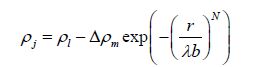
where ρj = plume/jet density; ρl = ambient liquid (water) density. λ= the spreading ratio that is defined as the ratio between the radius of the gas core and the total plume radius, $\Delta {{\rho }_{m}}$= difference between the density at the centerline of the plume and the ambient liquid density. Since a large amount of gas remains at the center region of the plume at stagnant ambient conditions, it is reasonable to assume that $\Delta {{\rho }_{m}}\approx {{\rho }_{l}}-{{\rho }_{g}}$ ; where ρg is the gas density. The void fraction for the gas jet/plume is $\varepsilon =\left( {{\rho }_{l}}-{{\rho }_{j}} \right)/({{\rho }_{l}}-{{\rho }_{g}})$ which can be expressed as $\varepsilon =\exp \left( -{{\left( \frac{r}{\lambda b} \right)}^{N}} \right)$ by re-arranging Eq.(2).
The governing equations are derived by applying the Reynolds transport theorem over a selected Eulerian control volume as shown in Fig. 1. The control volume starts from the release port up to a desired height below the ZFE. We use the control volume approach to reduce the mathematical complexities caused by the super Gaussian profiles.

|
| Figure 1 Schematic of an underwater gas release |
We assume steady state conditions and constant ambient liquid density within the range of ZFE. By applying Reynolds Transport Theorem, mass conservation of liquid phase for a selected control volume can be derived as
|
(3) |
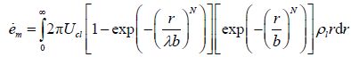
where ${{\dot{e}}_{m}}$ = liquid mass entrained into the plume due to shear. The ambient liquid entrainment into the plume due to gas velocity is small compared to the ambient liquid entrainment due to the plume-liquid velocity (Husssain and Siegel, 1976). Furthermore, the entrained liquid mass is proportional to the surface area of the control volume. Therefore ${{\dot{e}}_{m}}$ is evaluated as, $N=f\left( {}^{1}\!\!\diagup\!\!{}_{{{\left( {}^{z}\!\!\diagup\!\!{}_{{{D}_{0}}}\; \right)}^{k}}}\;,F{{r}_{0}} \right)$ , where z = vertical distance: $\alpha $ = entrainment coefficient. After integrating and substituting for ${{\dot{e}}_{m}}$ , Eq.(3) reduces to a non-dimensional form as

|
(4) |
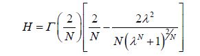
where $B=b/{{b}_{0}}$ = non-dimensional plume radius; b0 = radius of the release port. Here H is evaluated as
|
(5) |
where $\Gamma $ = Gamma function, N= shape factor for the super Gaussian profile.
2.2 Momentum conservation for the liquid phaseThe upward momentum on the liquid is induced by the drag force created by the moving gas bubbles (Hussain and Narang, 1984; Delnoij et al., 1997). Momentum conservation for the liquid phase can be expressed as

|
(6) |
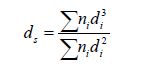
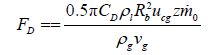
where FD= drag force acting on the liquid mass by the moving gas bubbles. For simplicity, the gas bubbles are assumed to be solid spheres in the analysis (Delnoij et al., 1997). According to Delnoij et al.(1997) the drag force acting on the liquid by a single gas bubble (fd) can be evaluated as, ${{f}_{d}}=0.5\text{ }\!\!\pi\!\!\text{ }{{C}_{D}}{{\rho }_{l}}R_{b}^{2}{{\left| {{u}_{r}} \right|}^{2}}$. Here, CD = drag coefficient between the liquid phase and gas bubble; Rb= mean radius of a gas bubble. If gas bubbles are distributed over a wide range of diameters, we recommend using radius corresponding to Sauter mean diameter (ds) for Rb, which is given by
|
(7) |
where ni = number concentration of ith bubble diameter class; di = corresponding diameter of theith bubble diameter class. ur is the relative velocity between the liquid phase and the moving gas bubbles, which is approximately equal to ${{u}_{cg}}$.${{u}_{cg}}$ is the gas velocity at the plume/jet axis and it is approximated as, ${{u}_{cg}}\approx {{U}_{0}}+{{u}_{b}}$ where, ${{U}_{0}}$ is the near source gas release velocity and is the buoyant velocity of the gas bubbles. Then the total drag force acting on the liquid phase can be expressed as
|
(8) |
where $\dot{m}0$ = the mass flowrate of gas at source; vg= volume of a gas bubble of mean diameter. By integrating Eq.(6) and substituting from Eq.(8) the momentum conservation equation can be simplified to a non-dimensional form as
|
(9) |
Solving Eq.(4) and Eq.(9) simultaneously gives the non-dimensional liquid velocity at the plume axis at a height z as
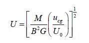
|
(10) |
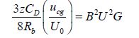
where M and G are calculated as
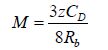
|
(11) |

|
(12) |
Based on the derivation above, the plume centerline velocity and the plume width in the developing flow region of the plume can be expressed using Eqs.(4), (9), (10), (11) and (12). To completely define the NSP conditions we need to calculate the drag coefficient (CD, shape factor for velocity profile (N), and the entrainment coefficient (α). Due to lack of rigorous theoretical explanations for CD, N, and α, we propose semi-empirical equations to describe them based on physical experimental evidences.
3 Experimental dataDetailed experimental data for the ZFE of underwater gas releases are rare. Simiano (2005) contains comprehensive and useful data. The experiments were carried out in LINX (Large-scale Investigation of Natural circulation, condensation and miXing) facility in Switzerland which is equipped with modern instrumentation. The liquid and bubble velocity distributions inside the plume were measured using Particle Image Velocimetry (PIV). Then the radial distributions of averaged turbulent velocity profiles for the liquid phase at different heights were given. More details on the experimental procedure and parameters can be found in Dhotre and Smith (2007) . Some of the key experimental parameters are given in Table 1. The experimental data are shown along with the model results in the next section.
| Parameter | Value |
| Air mass flow rate/ (Nliter·s−1) | 0.125, 0.25 |
| Immersion depth/m | 1.5 |
| Injector plate diameter/m | 0.15 |
| Vessel diameter/m | 2.0 |
| Averaged bubble sizes/mm | 2-3 |
| *Nliter = Normalized Liter | |
This section describes the calibration and verification of the method developed in this paper using the experimental data from Simiano (2005) . The parameters CD, N, and α in the formulation need to be modeled empirically with physical insight, since they are too complex to evaluate theoretically alone. Therefore, a few selected experiments are used to calibrate the model and the others are used to validate the model. Figs. 2 (a) - (d) show the comparison between the computed values and the experimental data used for calibration of the model. Model verification with experimental data are shown in Figs. 3-5. These figures show nine subplots which include comparisons with experimental data.
According to Delnoij et al.(1997) CD can be determined based on the Reynolds number as suggested by Clift et al.(1978) . Delnoij et al.(1997) emphasizes that the drag predicted as in Clift et al.(1978) varies from the actual values in practical situations. The drag force is expected to vary in the ZFE where the liquid flow is accelerated (as shown experimentally in Simiano, 2005) and the drag force becomes constant at the end of the ZFE. One reason for this variation in the drag force is the bubble break up and coalescence. Bubble break up and coalescence occur extensively within the ZFE and gradually diminish at the end of ZFE (Bandara and Yapa, 2011) which causes the drag force to reach a nearly constant value. This variation of drag force can be best represented by expressing CD as a function of shape index N. Therefore, an expression for CD is proposed as

|
(13) |
The shape index - N is the parameter that defines the shape of the velocity profile in the developing flow region. The velocity profile should change from top-hat to Gaussian. Here, the gas release conditions and the non-dimensional distance along the plume centerline are identified as key variables that affect the velocity profile for a particular height z. Thus N can be expressed as a function of the release Froude number and non-dimensional vertical distance. N can be expressed in functional form as $N=f\left( {}^{1}\!\!\diagup\!\!{}_{{{\left( {}^{z}\!\!\diagup\!\!{}_{{{D}_{0}}}\; \right)}^{k}}}\;,\text{ }F{{r}_{0}} \right)$ where the functional form has to be decided based on experimental data. Then using the data in Fig. 2 (a) to (d) an expression is formed for N as
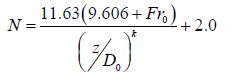
|
(14) |

|
| Figure 2 Radial velocity distribution against experimental data for an air flow rate of 0.125 L/s |
where Fr0= Froude number of gas flow at the release port ; D0= diameter of the release port. N is expected to be a large number, representing a top hat profile, at the beginning and N=2, representing a Gaussian profile at the end of the ZFE region. This can be achieved by selecting the appropriate value for k. Earlier studies have shown that the length of ZFE has to be roughly varied between 5D0 to 10D0. According to our calculations, k=4 gives a large value for N at the beginning and asymptotically reach 2 while ZFE is around 5D0. Thus, k=4 is suggested.
Previous studies on the behavior of entrainment coefficient in ZFE for underwater gas releases are extremely rare. According to Hill (1972) , the entrainment coefficient in the near source region of an underwater gas release varies with vertical distance. Falcone and Cataldo (2003) also conducted an experiment to study the entrainment coefficient in the near source region of a horizontal pure liquid jet. They also presented an empirical relation for the entrainment coefficient in the near source region as a function of non-dimensional vertical distance. Based on the work done by Hill (1972) and Falcone and Cataldo (2003) the entrainment coefficient is formulated as a function of non-dimensional vertical distance given by

|
(15) |
Experimental conditions given in Dhotre and Smith (2007) and Simiano (2005) are simulated using the newly developed computational model, so that computational results can be compared with the experimental values. The liquid velocity profiles computed at different heights for different air flow rates are compared with the experimental data, as shown in Figs. 3-5. Empirical coefficients and relations remain constant throughout all the simulations described here. In all the figures US is referred to as the vertical liquid velocity at a specific radial distance for a given plume section.

|
| Figure 3 Radial velocity distribution against experimental data for an air flow rate of 0.125 L/s |
From Figs. 3 and 4, it is clear that the liquid velocity profiles change from top hat to Gaussian with the increase of distance from the release point. During this transition of velocity profiles, the mean liquid velocity increases gradually. This acceleration of the liquid is caused by the drag force acting on the liquid by the moving gas with a high momentum. All the plots in Fig. 3 show a good agreement with the experimental data. This implies that the super Gaussian profile can clearly represent the variation of velocity distribution mathematically. This fact is further consolidated by the plots in Fig. 4, which are for a different air flowrate (15 L/s). In Fig. 4 plots Fig. 4(a), (b), and (c) show a good agreement with experimental data while plots (d), (e), and (f) show an acceptable agreement with marginal deviations. It must be stated that the coefficients in the empirical relations are kept the same (fixed) for all the cases presented in this paper.

|
| Figure 4 Radial velocity distribution against experimental data for an air flowrate of 0.25 L/s |
The reason for these discrepancies is that the immersion depth is not relatively large enough, compared to the diameter of the injector plate to avoid the circulation of liquid jet induced by the gas flow. This internal flow circulation affects the entrainment process and makes it more complex. Since stagnant ambient conditions are assumed and disregarded the circulation effects in the theoretical model, the computed data estimates higher liquid velocities compared to the measured data.
In spite of the short comings described above, the suggested method simulates the near source velocity profiles well enough for different flow conditions. Since the plume heights which have been considered for data gathering are very close to the release port, it is not possible to observe a significant growth of plume radius. Therefore, comparisons for B are not relevant for the presented study. However, the most important parameter to decide the plume velocity near the source is the liquid velocity of the plume axis at the desired height. It is important that we calculate the liquid velocity at the plume axis with reasonable accuracy. Fig. 5 (a) and (b) shows the comparison of non-dimensional velocity at the plume axis at different heights of the plume for two different gas flowrates (7.5 L/s and 15 L/s). The computed liquid velocities at the plume axis match well with the measured data for two different air flowrates.

|
| Figure 5 Center line velocity at different plume heights against experimental data |
This paper developed a new way to model the time averaged velocity and density variations during the early stage of an underwater gas release. The core part of the work depends on the analytical equations (Eqs.(1) to (12) )which mathematically represent the plume behavior near the source. To close the equations developed based on the physical laws (i.e. Eqs.(1) to (12) )the three semi-empirical parameters (CD, N, and α) should be evaluated. Eqs.(13) to (15) are introduced to compute those parameters. These empirical relations can be further strengthened in the future if more data becomes available.
The major application of this new work is to determine accurate NSP conditions for underwater gas releases. This will help future comprehensive simulations of gas transport and fate in two ways: i) more accurate calculation of gas bubble size distribution; ii) completely automated simulation (transport and fate) of underwater gas releases.
Simiano’s (2005) experimental data are used to validate the suggested model. One set of experimental data consisting of 4 experiments was used to evaluate the three empirical coefficients. Then a different set of data that consist of 9 experiments were used to test and validate the developed model.
In the comparisons, the computed data matches well with the measured data, with small deviations in higher air flowrates. Since the experiment was conducted in a closed vessel it is unavoidable to have internal flow circulations within the vessel specifically for higher gas flowrates. But actual underwater gas releases occur in infinite fluid domains, where the suggested modeling approach is expected to work well even for higher flowrates. Further, the comparisons illustrates that the proposed mathematical model can successfully simulate the transitions of liquid velocity profiles from Top hat to Gaussian in the ZFE region. The liquid velocity increases until the liquid plume is fully developed at the height where the radial velocity distribution becomes approximately Gaussian (N≈2.0 to 2.3). A bubble plume model which begins numerical integration at the end of the ZFE, can be fed with the liquid velocity computed when N≈2.0 to 2.3 (approximately Gaussian) as the near source velocity of the plume. The other significance is that, the proposed method is applicable to estimate the approximate length of the ZFE for a particular underwater gas release.
| Bandara UC, Yapa PD, 2011. Bubble sizes, breakup, and coalescence in deepwater gas/oil plumes. Journal of Hydraulic Engineering, 137(7), 729–738. DOI:10.1061/(ASCE)HY.1943-7900.0000380 |
| Cederwall K, Ditmars JD, 1970. Analysis of air-bubble plumes. KH-R-24. W. M. Keck Laboratory of Hydraulics and Water Resources, Division of Engineering and Applied Science, California Institute of Technology. |
| Clift R, Grace JR, Weber ME, 1978. Bubbles, drops, and particles. Academic Press, New York, USA. |
| Cloete S, Olsen JE, Skjetne P, 2009. CFD modeling of plume and free surface behavior resulting from a sub-sea gas release. Applied Ocean Research, 31, 220–225. DOI:10.1016/j.apor.2009.09.005 |
| Delnoij E, Lammers FA, Kuipers JAM, van Swaaij WPM, 1997. Dynamic simulation of dispersed gas-liquid two-phase flow using a discrete bubble model. Chemical Engineering Science, 52(9), 1429–1458. DOI:10.1016/S0009-2509(96)00515-5 |
| Dhotre MT, Smith BL, 2007. CFD simulation of large-scale bubble plumes: Comparisons against experiments. Chemical Engineering Science, 62(23), 6615–6630. DOI:10.1016/j.ces.2007.08.003 |
| Drew B, Charonko J, Vlachos P, 2011. Liquid entrainment by round turbulent gas jets submerged in water. ASME-JSME-KSME 2011 Joint Fluids Engineering Conference, 2723-2731. DOI: 10.1115/AJK2011-11015 |
| Fabregat A, Dewar WK, Ozgonkmen TM, Poje AC, Wienders N, 2015. Numerical simulations of turbulent thermal, bubble and hybrid plumes. Ocean Modelling, 90, 16-28. DOI: 10.1016/j.ocemod.2015.03.007 |
| Falcone AM, Cataldo JC, 2003. Entrainment velocity in an axisymmetric turbulent jet. Journal of Fluids Engineering, 125(4), 620–627. DOI:10.1115/1.1595674 |
| Fannelop T, Sjoen K, 2015. Hydrodynamics of underwater blowouts. 18th Aerospace Sciences Meeting. [2015-05-13], http://arc.aiaa.org/doi/abs/10.2514/6.1980-219. |
| Ferentinos, J. Infield System, 2013. Global offshore oil and gas outlook. Presented at the Gas/Electric Partnership. |
| Hill BJ, 1972. Measurement of local entrainment rate in the initial region of axisymmetric turbulent air jets. Journal of Fluid Mechanics, 51(4), 773–779. DOI:10.1017/S0022112072001351 |
| Hirst E, 1971. Analysis of buoyant jets within the zone of flow establishment. Oak Ridge National Lab, ORNL technical report No. ORNL-TM--3470. |
| Hussain NA, Narang BS, 1984. Simplified analysis of air-bubble plumes in moderately stratified environments. Journal of Heat Transfer, 106(3), 543–551. DOI:10.1115/1.3246713 |
| Hussain NA, Siegel R, 1976. Liquid jet pumped by rising gas bubbles. Journal of Fluids Engineering, 98(1), 49–56. DOI:10.1115/1.3448206 |
| Johansen Ø, 2000. DeepBlow-a Lagrangian plume model for deep water blowouts. Spill Science & Technology Bulletin, 6(2), 103–111. DOI:10.1016/S1353-2561(00)00042-6 |
| Kobus HE, 1968. Analysis of the flow induced by air-bubble systems. Coastal Engineering Conference, London, 2, 1016-1031. |
| Lima Neto IE, 2012. Modeling the liquid volume flux in bubbly jets using a simple integral approach. Journal of Hydraulic Engineering, 138(2), 210–215. DOI:10.1061/(ASCE)HY.1943-7900.0000499 |
| Liro CR, Adams EE, Herzog HJ, 1991. Modeling the release of CO2 in the deep ocean. Energy Laboratory, Massachusetts Institute of Technology, Cambridge, Technical Report No. MIT-EL 91-002. |
| McDougall TJ, 1978. Bubble plumes in stratified environments. Journal of Fluid Mechanics, 85(4), 655–672. DOI:10.1017/S0022112078000841 |
| McGinnis DF, Lorke A, Wüest A, Stöckli A, Little JC, 2004. Interaction between a bubble plume and the near field in a stratified lake. Water Resources Research, 40(10), W10206. DOI:10.1029/2004WR003038 |
| Milgram JH, 1983. Mean flow in round bubble plumes. Journal of Fluid Mechanics, 133, 345–376. DOI:10.1017/S0022112083001950 |
| Mudde RF, Simonin O, 1999. Two- and three-dimensional simulations of a bubble plume using a two-fluid model. Chemical Engineering Science, 54(21), 5061–5069. DOI:10.1016/S0009-2509(99)00234-1 |
| Nissanka ID, Yapa PD, 2016. Calculation of oil droplet size distribution in an underwater oil well blowout. Journal of Hydraulic Research (IAHR), 54(3), 307–320. DOI:10.1080/0221686.2016.1144656 |
| Olsen JE, Skjetne P, 2016. Current understanding of subsea gas releases: A review. Canadian Journal of Chemical Engineering, 94, 209–219. DOI:10.1002/cjce.22345 |
| Shealy DL, Hoffnagle JA, 2006. Beam shaping profiles and propagation. Applied Optics, 45(21), 5118–5131. DOI:10.1117/12.619305 |
| Simiano M, 2005. Experimental investigation of large-scale three dimensional bubble plume dynamics. PhD thesis, Swiss Federal Institute of Technology, Zurich. |
| Simiano M, Zboray R, Cachard F de, Lakehal D, Yadigaroglu G, 2006. Comprehensive experimental investigation of the hydrodynamics of large-scale, 3D, oscillating bubble plumes. International Journal of Multiphase Flow, 32(10-11), 1160–1181. DOI:10.1016/j.ijmultiphaseflow.2006.05.014 |
| Smith BL, 1998. On the modelling of bubble plumes in a liquid pool. Applied Mathematical Modelling, 22(10), 773–797. DOI:10.1016/S0307-904X(98)10023-9 |
| Socolofsky SA, Bhaumik T, Seol D, 2008. Double-plume integral models for near-field mixing in multiphase plumes. Journal of Hydraulic Engineering, 134(6), 772–783. DOI:10.1061/(ASCE)0733-9429(2008)134:6(772) |
| Sokolichin A, Eigenberger G, Lapin A, 2004. Simulation of buoyancy driven bubbly flow: Established simplifications and open questions. American Institute of Chemical Engineers Journal, 50(1), 24–45. DOI:10.1002/aic.10003 |
| U.S. Energy Information Administration (US EIA), 2014. Brazil. International energy data and analysis. https://www.eia.gov/beta/ international/analysis_includes/countries_long/Brazil/brazil.pdf. |
| Wüest A, Brooks NH, Imboden DM, 1992. Bubble plume modeling for lake restoration. Water Resources Research, 28(12), 3235–3250. DOI:10.1029/92WR01681 |
| Yapa PD, Dasanayaka LK, Bandara UC, Nakata K, 2010. A model to simulate the transport and fate of gas and hydrates released in deepwater. Journal of Hydraulic Research, 48(5), 559–572. DOI:10.1080/00221686.2010.507010 |
| Zhao L, Boufadel MC, Socolofsky SA, Adams E, King T, Lee K, 2014. Evolution of droplets in subsea oil and gas blowouts: Development and validation of the numerical model VDROP-J. Marine Pollution Bulletin, 83(1), 58–69. DOI:10.1016/j.marpolbul.2014.04.020 |
| Zheng L, Yapa PD, Chen F, 2003. A model for simulating deepwater oil and gas blowouts - Part I: theory and model formulation. Journal of Hydraulic Research, 41(4), 339–351. DOI:10.1080/00221680309499980 |