2. Fujian Province Key Laboratory of Structural Performances in Ship and Ocean Engineering, Fuzhou 350116, China
1 Introduction
Ship maneuverability is one of the most important indicators of the hydrodynamic performance of a ship. In fact, the prediction of ship maneuverability at the ship design stage is explicitly required by current Standards for Ship Maneuverability (IMO, 2002). Computer simulation based on a mathematical model of ship maneuvering motion provides an effective way to predict ship maneuverability. However, using this method requires the determination of the model parameters. The accuracy of prediction depends on the accuracy of the model parameters, which usually refer to the hydrodynamic coefficients. In the past, several approaches have been proposed to determine the hydrodynamic coefficients, including the database- dependent method, empirical formulas, captive model test, theoretical or numerical calculation (Computational Fluid Dynamics, CFD), and System Identification (SI) combined with free-running model tests. Of these, the SI-based approach has been proven as an effective and practical method (Sutulo and Guedes Soares, 2014).
During the last decades, many authors have proposed different approaches to identify the hydrodynamic coefficients in the mathematical model of ship maneuvering. For example, Holzhüter (1989) proposed a robust identification based on Least Squares (LS) in autopilot design. Yoon and Rhee (2003) applied the ridge regression method that features Estimation-Before-Modeling to identify hydrodynamic derivatives. Van Amerongen (1984) addressed the application of Model Reference Method (MRM) to ship steering. Abkowitz (1980) applied the Extended Kalman Filter (EKF) to identify ship maneuvering motion. Källström and ström (1981) presented the application of Maximum Likelihood (ML) to ship steering. Zhou and Blanke (1989) used the Recursive Prediction Error (RPE) to identify a class of nonlinear ship maneuvering models. Bhattacharyya and Haddara (2006) proposed Fourier Transformation (FT) to identify ship maneuvering models, whereas Chen et al.(2010) presented the use of Particle Swarm Optimization (PSO) to the parametric identification of ship maneuvering. Herrero and Gonzalez (2012) applied the unscented Kalman filter to the identification of nonlinear manoeuvring models. Luo et al.(2014) proposed an approach based on Support Vector Machines (SVM) to the identification of ship maneuvering motion.
Generally, those identification methods mentioned above can be categorized as “iteration-based identification” (e.g., LS, MRM, EKF, ML, RPE, PSO) and “iteration-free identification” (e.g., FT, SVM) methods. More often, the iteration-based identification is preferable in studying ship maneuvering. The most commonly used method in the identification of model parameters in a ship maneuvering model is the LS method, which adopts iterative processes. For the iteration-based identification, the initial estimation of hydrodynamic coefficients is typically required, because such estimation exerts an important influence on the identification results. However, it is difficult to theoretically select the appropriate initial coefficients. In many cases, the initial values of coefficients are determined by trials.
Haddara and Wang (1999) proposed the Back Propagation Neural Network (BPNN) in identifying the parameters of a hydrodynamic model of ship maneuvering motion. However, NN was actually only used to approximate the nonlinear hydrodynamic forces and moment. Afterwards, LS-based regression was applied to obtain the hydrodynamic coefficients contained in the models of nonlinear hydrodynamic forces and moment. Ebada and Abdel-Maksoud (2005) also utilized the black-box modeling ability of NN (rather than the parametric identification approach proposed in this paper), and proposed the BPNN to predict the limits of ship turning circle maneuvers. Moreira and Guedes Soares (2003a; 2003b) applied the recursive NNs to ship maneuverability prediction and maneuvering motion simulation. Hess et al.(2006) studied the online prediction of ship maneuvering by using dynamical recursive NNs. Rajesh and Bhattacharyya (2008) addressed the blind prediction of ship maneuvering by using multilayer feed forward NNs.
In this paper, the use of Neural Networks (NNs) is proposed to achieve the parametric identification of ship maneuvering models. An online two-layer feed forward NN is adopted, and a nonlinear response model is investigated along with a linear hydrodynamic model of ship maneuvering motion. The maneuverability indices and linear non-dimensional hydrodynamic derivatives in the models are approximated by the weights in the NN. Unlike the conventional iteration-based algorithms, no initial estimation of the model parameters is required in the proposed model. The initial values of the parameters can also be set freely, e.g., zeros.
2 Mathematical model of ship maneuvering motionTo predict the ship maneuvering motion, two kinds of maneuvering models can be used. One is the hydrodynamic model, including the Abkowitz model and the Mathematical Modeling Group (MMG) model, and the other is the response model. The hydrodynamic model typically features many hydrodynamic derivatives, and some of them are difficult to determine accurately, especially for nonlinear derivatives. Comparatively, the response model, or the so-called Nomoto model, is preferred in practical applications owing to its simple structure, which reflects a ship's responses (e.g., velocities, angular velocity) to given controls (e.g., rudder angle). Moreover, this kind of model is commonly used in the ship autopilot design.
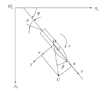
Usually, the motion of a ship can be described in a six-degree-of-freedom frame, including surge, sway, yaw, heave, pitch, and roll. From the point of view of maneuvering prediction, attention is often paid to the ship's motion in the horizontal plane instead of the vertical plane. In other words, only surge, sway, and yaw are often considered. Fig. 1 depicts the ship maneuvering motion for a surface ship. The inertial coordinate system is denoted by ${x_0}{o_0}{y_0}$, $xoy$ is the attached coordinate system, G the center of gravity, u the surge speed, v the sway speed, r the yaw rate, U the total velocity, d the rudder angle, y the heading angle, and β the drift angle.
The linearized equations of ship maneuvering motion can be expressed as

|
(1) |
where m denotes the mass of the ship; Iz is the inertia moment with respect to the z-axis (in the attached coordinate system, pointing to the center of the Earth)
Suppose the perturbation of the surge speed is small, i.e., $\Delta u \approx 0$, the first equation in can be removed. Therefore, it follows that

|
(2) |
It should be noted that only sway and yaw motions are considered in Eq.(2) Compared with Eq.(1) . Such a simplification is reasonable, because (i) the equation of surge motion is decoupled from the equations of sway and yaw motions; and (ii) from the point of view of ship maneuverability, greater attention is given to the sway and yaw motions than the surge motion, because the rudder at the stern exerts an influence on the former, but only little influence on the latter, as shown in Eq. (1).
By applying Laplace transformation to the above equations, the transfer functions from the rudder angle (δ) to the yaw rate (r) and sway speed (v) can be respectively obtained as

|
(3) |

|
(4) |
From the point of view of practical helm, greater attention is usually given by researchers to the yaw than the sway motion. Moreover, measuring the heading angle or yaw rate (r) is much easier than measuring sway velocity. Therefore, the response model of yaw motion is commonly used, both in studies on prediction of ship maneuvering and autopilot design.
Ship motion is usually characterized by large inertia and low frequency. Consequently, the transfer function from the rudder angle to the yaw rate can be described as

|
(5) |
By using inverse Laplace transformation, the first-order linear response model with respect to the yaw motion in the time domain can be described as

|
(6) |
where T and K are the maneuverability indices, which can be expressed by the hydrodynamic derivatives respectively given by

|
In consideration of the variation of the surge speed and the nonlinear characteristic of the surrounding flow, the dynamics of ship motion is essentially nonlinear. Based on the linear response model, if nonlinear dynamics is taken into account, the following first-order nonlinear response model can be obtained

|
(7) |
where α is the coefficient of the nonlinear term (Nomoto et al., 1957).
|
| Figure 1 Coordinate system of ship maneuvering motion |
The current paper studies the identification of the linear hydrodynamic model described by Eq.(2) and the nonlinear response model shown in Eq.(7). Taking the identification of response model as an example, rewriting Eq.(7) yields

|
(8) |
Denote

|
(9) |
A two-layer feed forward NN is used to approximate the above nonlinear system, with the form expressed as

|
(10) |
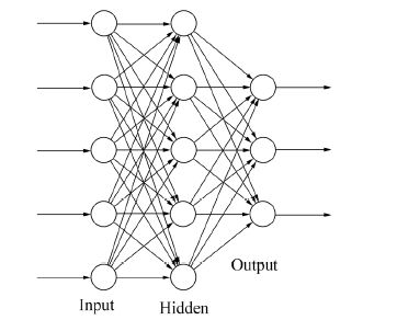
where W is the weight vector, Φ is the activation function vector, and ε is the approximation error (Lewis et al., 1995). If the error is small enough, W can be called “ideal” weight and satisfies ${\left\| {W} \right\|_{F}} \le {W_{M}}$ (${W_{M}}$ is a positive constant). Here, ${\left\| \cdot \right\|_{F}}$ represents the Frobenius norm (F-norm). Fig. 2 depicts a structure of three-layer feedforward NN. When the weights between the input and hidden layers are set to constants, such a network can be defined as the so-called two-layer feed forward NN. During the last two decades, this kind of NN has found wide applications in many areas, especially in cybernetics. In this paper, this kind of NN is introduced to the parametric identification of a nonlinear dynamic system, i.e., the ship maneuvering motion.
|
| Figure 2 Feed forward neural network |
Based on the two-layer feed forward NN, an estimation of the “ideal” weight leads to the estimation of $\dot r(t)$

|
(11) |
where We is the estimate of W.
By reference to Eq.(8), We and Φ can be defined respectively as

|
where ${\hat \alpha _1},{\hat \beta _1},{\hat \gamma _1}$ are the estimates of ${\alpha _1},{\beta _1},{\gamma _1}$.
Define

|
the online algorithm of Wecan be designed as

|
(12) |
where k1, 2, 3 > 0, $\left\| \cdot \right\|$ represents the Euclidian norm.
3.2 Convergence of estimationLet a candidate Lyapunov function

|
(13) |
where the weight error, ${\tilde W} = {W} - {{W}_e}$ tr{·} denotes the trace of a matrix. The derivative of Eq.(13) is given by

|
(14) |
If $0 < a < 1$, then one has

|
(15) |
Let, $\mu = \min \left\{ {(1 - a){k_1}/{k_2},\;(1 - a){k_3}\left\| {\xi } \right\|} \right\}$ then one has

|
(16) |
Through the appropriate selection of NN parameters, i.e., k1, 2, 3, it holds that

|
(17) |
Then one has

|
(18) |
We can prove that the error system $(e,{\tilde W})$ is Uniformly Ultimately Bounded (UUB) stable (Qu and Dawson, 1995). Furthermore, a small ${\tilde W}$ indicates that the estimates of ${\alpha _1},{\rm{ }}{\beta _1},{\rm{ }}{\gamma _1}$ approximate their true values well.
4 Prediction of ship maneuveringIn order to create a response model, the sample is taken from the 20°/20° zigzag maneuver tests of a model ship. The tests were conducted in the seakeeping basin of the State Key Laboratory of Ocean Engineering in Shanghai Jiao Tong University. The principal particulars of the ship model are as follows: length of the model is L=3.16 m, draft is d=0.159 m, the block coefficient Cb is 0.85, the service speed is v=1.2 m/s, and the model scale is 1:50.
In order to remove the noisy data from the sample, a zero-phase digital filter is employed in preprocessing the sample. The transfer function is designed as

|
(19) |
with the complex poles $(0.5715,\; \pm 0.2936i)$.
The filtered results are shown in Fig. 3. As can be seen, few noises can be found in the sample. The filtered sample is then used in the identification of maneuverability indices.

|
| Figure 3 Filtering of test data |
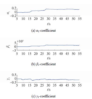
The parameters in NN are selected as follows: k1= k2=15, k3=0.5. The initial values of weight are set to zeros. Fig. 4 presents the approximation results, which indicate that the estimates agree well with the test results. Fig. 5 presents the histories of three parameters, i.e., ${\alpha _1},{\rm{ }}{\beta _1},{\rm{ }}{\gamma _1}$. As can be seen, the UUB stability is guaranteed. After calculating the expectations of ${\alpha _1},{\rm{ }}{\beta _1},{\rm{ }}{\gamma _1}$, the parameters in Eq.(7) can be determined as

|

|
| Figure 4 Approximation results by NN |
|
| Figure 5 Parametric histories |
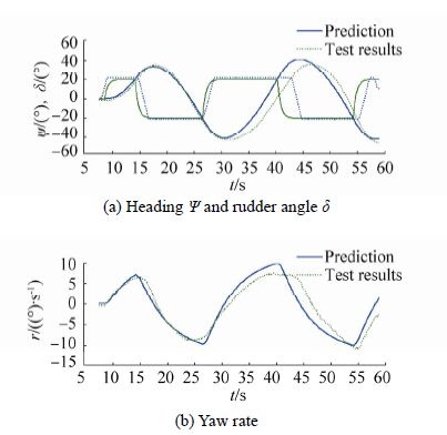
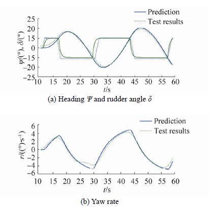
Based on Eq.(7), 20°/20° and 10°/10° zigzag maneuvers are predicted and compared with the model test results shown in Fig. 6 and Fig. 7 respectively, in which the heading angle is calculated by

|
(20) |
|
| Figure 6 Prediction results of 20°/20° zigzag maneuver |
|
| Figure 7 Prediction results of 10°/10° zigzag maneuver |
Checking the validity of the obtained maneuvering model based on NN identification is conducted not only by using the same data used for training (i.e., 20°/20° zigzag maneuver), but also by testing against another maneuver (10°/10° zigzag maneuver). As can been seen from the comparison, the predicted results agree well with the test results, especially for the prediction of the first and second overshoot angles. These findings thus demonstrate the validity of the proposed NN-based modeling method.
Further verification is performed with respect to the linear hydrodynamic model given by Eq. (2); its non-dimensional form is given by

|
(21) |
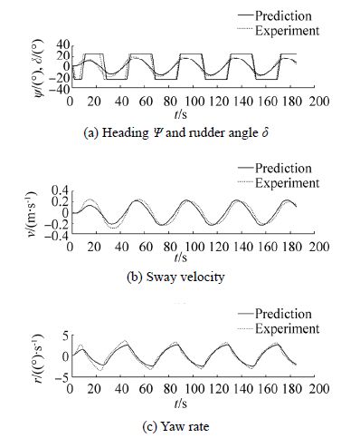
Data samples are taken from the 25°/5° zigzag maneuver test of the KVLCC2 ship model. The sampling was carried out at the Hamburg Ship Model Basin (HSVA). Details about the ship model and the experiment conditions can be found in (Luo et al., 2016). By applying NN to identify the non-dimensional hydrodynamic derivatives in, the parameters in the algorithm are set as follows: k1= 3×10⁻³, k2 =3×10⁻², k3 =4×10⁻⁴. Assuming that the initial values of the hydrodynamic derivatives are zeros, then the identification results are
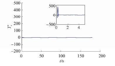
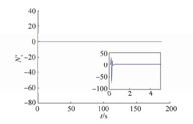
The added masses and added inertia of moment in are not identified because of the parameter identifiability (Abkowitz, 1980). Slender body theory provides simple formulae to estimate these parameters (Newman, 1977). Numerical simulation is performed by using the obtained hydrodynamic derivatives. Results are shown in Fig. 8. Meanwhile, in Figs. 9-14, the histories of the identified hydrodynamic derivatives are also presented. The embedded small plots in the Figs. 9-14 reflect the variations of the parameters at the initial stages.
|
| Figure 8 Prediction of 25°/5° zigzag maneuver of KVLCC2 |
|
| Figure 9 Histories of the parameters |

|
| Figure 10 Histories of the parameters |

|
| Figure 11 Histories of the parameters |
|
| Figure 12 Histories of the parameters |
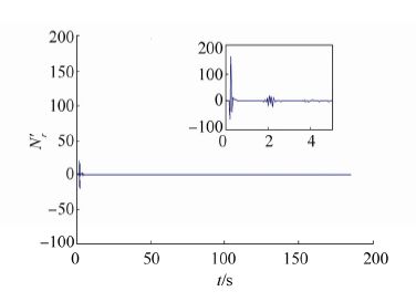
|
| Figure 13 Histories of the parameters |

|
| Figure 14 Histories of the parameters |
As shown by the simulation results, the prediction results agree well with the experimental results. Moreover, the stability of hydrodynamic derivatives is achieved.
5 ConclusionsNNs are proposed in the parametric identification of the mathematical models of ship maneuvering motion. The maneuvering indices and the linear hydrodynamic derivatives in the models can be estimated by the weights in the NNs. Using this method, no initial estimates of model parameters are required. The stability of estimation is also confirmed.
In the next work, more efforts will be devoted to improve the accuracy of parametric identification and propose a more sophisticated maneuvering model, such as an Abkowitz model or a nonlinear MMG model.
AcknowledgementThe authors are grateful to the Hamburg Ship Model Basin (HSVA) for providing the experimental data.
| Abkowitz MA, 1980. Measurement of hydrodynamic characteristic from ship maneuvering trials by system identification. Transactions of Society of Naval Architects and Marine Engineers, 88, 283–318. |
| Bhattacharyya SK, Haddara MR, 2006. Parametric identification for nonlinear ship manoeuvring. Journal of Ship Research, 50(3), 197–207. |
| Chen Y, Song Y, Chen M, 2010. Parameters identification for ship motion model based on particle swarm optimization. Kybernetes, 39(6), 871–880. DOI:10.1108/03684921011046636 |
| Ebada A, Abdel-Maksoud M, 2005. Applying artificial intelligence (A. I.) to predict the limits of ship turning manoeuvres. Year Book of Shipbuilding Institute, 99, 132–139. |
| Haddara MR, Wang Y, 1999. Parametric identification of maneuvering models for ships. International Shipbuilding Progress, 46(445), 5–27. DOI:10.3233/ISP-1999-4644501 |
| Herrero ER, Gonzalez FJV, 2012. Two-step identification of non-linear manoeuvring models of marine vessels. Ocean Engineering, 53, 72–82. DOI:10.1016/j.oceaneng.2012.07.010 |
| Hess D, Faller W, Lee J, Fu T, Ammeen E, 2006. Ship maneuvering simulation in wind and waves: a nonlinear time-domain approach using recursive neural networks. Proceedings of the 26th Symposium on Naval Hydrodynamics, Rome. |
| Holzhüter T, 1989. Robust identification in an adaptive track controller for ships. Proceedings of the 3rd IFAC Symposium on Adaptive Systems in Control and Signal Processing, Glasgow, 275–280. |
| IMO, 2002. Standards for ship manoeuvrability. Resolution MSC.137(76). International Maritime Organization, Lodon. |
| Källström CG, Åström KJ, 1981. Experiences of system identification applied to ship steering. Automatica, 17(1), 187–198. DOI:10.1016/0005-1098(81)90094-7 |
| Lewis FL, Liu K, Yesildirek A, 1995. Neural net robot controller with guaranteed tracking performance. IEEE Transactions on Neural Networks, 6(3), 703–715. DOI:10.1109/72.377975 |
| Luo WL, Moreira L, Guedes Soares C, 2014. Manoeuvring simulation of catamaran by using implicit models based on support vector machines. Ocean Engineering, 82, 150–159. DOI:10.1016/j.oceaneng.2014.03.008 |
| Luo WL, Guedes Soares C, Zou ZJ, 2016. Parameter identification of ship manoeuvring model based on support vector machines and particle swarm optimization. Journal of Offshore Mechanics Arctic Engineering, 138(3), 031101–1. DOI:10.1115/1.4032892 |
| Moreira L, Guedes Soares C, 2003a. Dynamic model of manoeuvrability using recursive neural networks. Ocean Engineering, 30(13), 1669–1697. DOI:10.1016/S0029-8018(02)00147-6 |
| Moreira L, Guedes Soares C, 2003b. Comparison between manoeuvring trials and simulations with recursive neural networks. Ship Technology Research, 50, 77–84. DOI:10.1179/str.2003.50.2.004 |
| Newman JN, 1977. Marine hydrodynamics. Cambridge, USA: M.I.T Press. |
| Nomoto K, Tagushi T, Honda K, Hirano S, 1957. On steering qualities of ships. International Shipbuilding Progress, 4(35), 354–370. |
| Qu ZH, Dawson DM, 1995. Robust tracking control of robot manipulators. Piscataway, USA: IEEE Press. |
| Rajesh G, Bhattacharyya SK, 2008. System identification for nonlinear maneuvering of large tankers using artificial neural network. Applied Ocean Research, 30(4), 256–263. DOI:10.1016/j.apor.2008.10.003 |
| Sutulo S, Guedes Soares C, 2014. An algorithm for offline identification of ship manoeuvring mathematical models from free-running tests. Ocean Engineering, 79, 10–25. DOI:10.1016/j.oceaneng.2014.01.007 |
| Van Amerongen J, 1984. Adaptive steering of ships - a model reference approach. Automatica, 20(1), 3–14. DOI:10.1016/0005-1098(84)90060-8 |
| Yoon HK, Rhee KP, 2003. Identification of hydrodynamic derivatives in ship maneuvering equations of motion by estimation-before-modeling technique. Ocean Engineering, 30, 2379–2404. DOI:10.1016/S0029-8018(03)00106-9 |
| Zhou WW, Blanke M, 1989. Identification of a class of nonlinear state-space models using RPE techniques. IEEE Transactions on Automatic Control, 34(3), 312–316. DOI:10.1109/9.16421 |


