


 , ,
, ,
2. Department of Ship Structural Design and Analysis, Technical University of Hamburg, Hamburg D-21073, Germany
1 Introduction
Arctic shipping means shipping in or through arctic waters. Its motivation might be to transport cargo between two or more arctic locations (intra-arctic shipping), to transport natural resources (e.g. oil and natural gas) from the Arctic to non-arctic markets (destination arctic shipping), or to reduce the transport distance between two or more non-arctic locations (trans-arctic shipping).
Safe and sustainable arctic shipping requires arctic ships, i.e. ships that are purposefully designed and built for arctic specific operating conditions. Arctic ships are generally exposed to sea ice and extreme weather conditions. Sea ice in particular has a very significant impact both on a ship’s resistance and the structural loads that it is exposed to. Therefore, when designing an arctic ship, it is necessary to carefully consider the ice conditions that the ship is expected to encounter. However, this is challenging as ice conditions are area specific and subject to large, and seemingly random annual and inter-annual variations. In addition, due to a lack of appropriate tools, it is difficult to relate ice conditions to structural loads and hull resistance (ISSC, 2015). Existing design rules do not help as they are prescriptive by nature and fail thereby to consider the actual operating conditions of a ship. Another factor that makes the design of arctic ships challenging is that they are often parts of complex transport systems including icebreakers (IBs) making it necessary to consider the wider context in which a ship operates.
Due to the expected increase in arctic shipping, there is a need for a design method that handles the above listed challenges in an adequate manner. In response to this need, we have developed a design method especially developed for arctic maritime transport systems. The method, which in the following is referred to as Simulation-Based Design (SBD), aims at finding a robust and cost-efficient transport solution that is adapted to the actual operating conditions. Towards this aim, it treats an arctic ship as a component integrated into a wider Arctic Maritime Transport System (AMTS) that might include loading and unloading ports, a fleet of other cargo ships, IBs, as well as Search and Rescue (SAR) and Oil Spill Response (OSR) resources. Design criteria are defined in terms of goals or risk criteria in accordance with the principles of Goal- and Risk-Based Design (GBD/RBD) as presented by Papanikolaou (2009) . Uncertain design parameters are defined in terms of either Probability Density Functions (PDF) or time series, and the resulting stochastic performance is estimated utilizing the technique of Discrete Event Simulation (DES).
The objective of the present paper is to apply SBD in a case study in order to assess its advantages over traditional design methods in which a ship is designed as a separate unit against a deterministic set of design parameters following prescriptive design rules. Specifically, the paper aims to answer the following research questions:
1) What additional information can be obtained by applying simulations and probabilistic design parameters in the design process?
2) What advantages can be obtained by system thinking, i.e., by extending the boundaries of the design task beyond the individual vessel?
Previous studies using simulations as a means to access the performance of arctic ships include Valkonen and Riska (2014) and Schartmüller et al.(2015) . The former presents a simulation-based tool referred to as COSSARC that can be used to assess the transit time of a ship operating in ice-infested waters. The latter presents a simulation-based design tool for arctic transport shipping that can be used to determine under what conditions the use of the Northern Sea Route is economically feasible. We are not aware of any other study investigating the merits of extending design boundaries in arctic ship design. However, the idea of extending design boundaries is not new as it is presented by Hagen and Grimstad (2010) , who conclude that any significant improvements in marine transport efficiency needs to come from a shift from “ship focus” to “transport system focus”. The novelty of the present study is that it 1) merges the concept of “transport system focus” and simulation-based performance assessment into a probabilistic design method for arctic sea transport systems, and 2) that it quantifies the merits of the method in a specific case.
A significant effort is dedicated to the determination of the vast number of design parameters required for the case study. We aim to determine all parameters as accurately as possible using publically available sources and state of the art knowledge. Identified gaps in the state of the art knowledge and available data are highlighted.
The paper is organized as follows: First, it provides a brief introduction to SBD. Second, it presents a case study in which the design method is applied. Third, it discusses the outcome of the case study and draws conclusions.
2 Simulation-based designThe SBD design process can be described as a series of sub-processes in accordance with the flowchart presented in Fig. 1. First, the design context including the design objectives as well as the probabilistic operating conditions are determined. Second, a number of alternative Concepts of Operations (CONOPS) representing various strategies (e.g. independent or IB assisted operation) to meet the design objectives are determined. Third, for each CONOPS, a preliminary AMTS design is determined in terms of a preliminary set of design parameters. Fourth, each preliminary AMTS design is divided into a number of manageable subsystems, each performing a specific function. Fifth, each subsystem of each preliminary AMTS design is designed taking design objectives as well as requirements and limitations set by other subsystems into account. GBD/RBD is applied where possible to adapt the solution to the actual operational conditions. In addition, probabilistic approaches are applied where possible in order to find the subsystem design that is the most likely to provide the best performance. A population of feasible AMTS designs is obtained once all the subsystems of all the determined preliminary AMTS designs have been designed. Sixth, the competing AMTS designs are compared based on a probabilistic performance assessment. The design process is finalized by selecting the design that provides the best expected overall performance.

|
| Figure 1 Process model for SBD |
The case study deals with the design of an AMTS for the transport of LNG from the Port of Sabetta (Russia) to the port of Zeebrugge (Belgium). The route, which is presented in Fig. 2, is approximately 2 600 nautical miles (NM) going through the North Sea, the Norwegian Sea, the Barents Sea, the Pechora Sea, and the South Kara Sea. In accordance with our reference system presented by Yamal LNG (2015) , the annual transport requirement is 16.5 million metric tonnes (MT). Assuming an LNG density of 450 kg/m3, this corresponds to a daily average transport demand of approx. 100 000 m3. Because the port-based LNG storage in Sabetta is limited, continuous round-the-year operation is required to avoid production stops caused by a lack of storage capacity. Any production stop is assumed to result in a very significant economic loss and should therefore be avoided. In other words, a high operational reliability is desired. Specifically, the system is to be designed for 100-year operating conditions, i.e. the worst operating conditions that are expected within a period of 100 years.
The objective of the design process is to obtain a cost-efficient and robust transport solution that meets existing rules and regulations. The level of robustness, i.e. the system’s ability to deal with variations in the operating conditions is of particular importance because the system is to be operated for a period of 25 years, during which significant fluctuations in factors such as fuel price, IB tariffs, and ice conditions are expected.
3.1.2 Modelling of environmental parametersApproximately within the period November-June, significant amounts of first-year ice may be present in both the Pechora Sea and the South Kara Sea. First-year ice does have a very significant impact on the performance of a ship as it significantly affects both its resistance and structural loads. Thus, when designing an AMTS, it is necessary to carefully consider the ice conditions along the planned route (s). However, this is challenging as first-year ice is highly heterogeneous and its characteristics (e.g. thickness and concentration) are subject to a significant level of uncertainty. In order to deal with the heterogeneousity, it is necessary to determine a simplified description of the ice cover. For this purpose, we apply the concept of equivalent ice thickness. The equivalent ice thickness, in the following referred to as heq, is practical because it describes the prevailing ice conditions in a single figure relating to the average thickness of all the ice features in the area. However, as pointed out by Riska (2009) , there is no single commonly accepted definition of heq. In the present paper we define heq in accordance with Eq.(1) (Riska, 2010)
|
(1) |
where t is level ice thickness (m), c is ice coverage, hr_avg is the average ridge keel draft (m), ρ is the average ridge density (1/km), and α is a dimensionless shape factor relating to the assumed average geometry of ridges.

|
| Figure 2 The route, voyage legs, and typical ice conditions along the route in April |
Level ice thickness (t) determines the prevailing level is thickness. It can be estimated based on ice data derived from satellite pictures, ice data from on-site measurements, or based on a combination of a sea ice growth model and climate (temperature) data. Satellite picture based ice condition reports are provided by for instance AARI (2015) , whose approximately biweekly ice condition reports describe the ice cover in the Arctic as ice free, nilas (0-10 cm), young ice (10-30 cm), first-year-ice (30-200 cm), or multi-year ice. In order to obtain a higher accuracy, on-site measurements might be applied. The most comprehensive publically available source of on-site measurements is provided by Romanov (1995) , which among others determines the minimum, mean, and maximum level ice thickness in April for various Arctic sea areas. In order to estimate the development (state) of the ice cover throughout the cold period, an ice growth model is useful. A well proven ice growth model is the so called Zubov’s equation, which can be used to estimate the level ice thickness based on the number of cumulative freezing degree days (dfd). An empirical version of the model is presented in Eq.(2).
|
(2) |
Inter-annual level ice thickness variations are generally assumed to be normally distributed with an annual peak value occurring in April (Romanov, 1995). Thus, the scenario (annual) specific maximum level ice thickness can be described in terms of its mean value and standard deviation for April. In addition, an area specific upper limit value can be determined based on the existing ice data.
The ice coverage (c) determines the percentage of the sea area that is ice covered. It can be determined based on data from satellite pictures and on-site measurements. Generally, the coverage is area and season specific (Romanov, 1995).
The ridge keel draft hr equals the total ridge height minus the sail height hs, i.e. the part of the ridge that is above water. The average ridge height hr_avg can be determined based on the level ice thickness and established based on normally distributed ratios between the level ice thickness and the average sail height hs_avg, and between hs_avg and hr_avg (Romanov, 1995).
The average ridge density determines the average number of ridges per km along a specific distance. It differs from region to region and can generally be considered exponentially distributed (Romanov, 1995). The ridge shape factor is used to determine the cross-section of a ridge based on its draft assuming ridges to have the shape of a triangle with a specific slope angle. Values for are proposed by various studies including Riska (2010) .
As described above, the concept of heq is based on the principle of averaging. This means that it fails to consider local ice features such as large individual ridges that might stop a ship. Thus, when using the principle of heq, the potential effect of large individual ridges needs to be considered separately (Valkonen and Riska, 2014). According to Leppäranta (2011) , the probability density function of the sail height hs (or keel draft) of individual ridges follows Eq.(3)
|
(3) |
where . This means that the sail height is exponentially distributed above a specific cut-off value . If both average sail height hs_avg and the ridge density ρ are known, we can estimate the number of ridges exceeding a specific limit height that a ship will encounter while traveling a specific distance. If the chosen limit height corresponds to the ridge penetration capability of the ship, i.e. the maximum ridge size that the ship can penetrate with a single ram, the obtained number of ridges equals the number of times the ship in question will be stopped by a large ridge.
Another factor that the concept of heq fails to consider is the effect of compressive ice. Compressive ice occurs when there is a driving force (e.g. wind or sea current) pushing the ice cover towards a boundary (e.g. shoreline) (Eriksson, 2009). According to Heideman (1996) , wind is the most important cause and where severe compression occurs, the direction of the compression coincides with that of the wind.
Compressive ice might cause a ship both significant added resistance and ice loads (Riska, 1995). Thus, it is considered one of the most hazardous factors for a ship operating in first-year ice (Eriksson, 2009). Compressive ice might occur along the route (Østreng et al., 1999). However, currently we have no means to determine its likelihood, magnitude, or duration. According to Russian statistics, the probability of encountering ice compression is 60% but this figure is not supported by actual experience (Heideman, 1996). In the Russian database, the compressive ice conditions are quantified by a 0-3 ball scale. However, it is not possible to link the ball unit to actual stresses in the ice field (Heideman, 1996). On the upside, at least in the Baltic Sea, compressive ice conditions are generally local, i.e. limited to a relatively small area, and quite short lived lasting only a few hours (Eriksson, 2009). In addition, there are means of short-term forecasting of compressive ice, which should reduce the risk of a ship ending up in an area of severe compressive conditions.
Due to frequent ship traffic, the route will feature sections of consolidated brash ice channels, which might be thicker and more difficult to penetrate than the surrounding natural ice cover. This should not be a problem on open sea where there is enough space for multiple parallel channels. However, locally the width of the fairway might be limited preventing multiple parallel channels. In such areas, additional ice management might be necessary to allow the ships to pass through.
In open water, environmental factors such as wind, waves, and sea currents might affect the performance of the ships. However, the impact of these factors is expected to be relatively small in comparison with that of sea ice. Thus, they are excluded from the present study.
3.1.3 Quantification of environmental parametersIn order to enable a quantitative description of the ice conditions along the route, we divide the route into three legs in accordance with Fig. 2. Leg 1 goes over the North Sea, the Norwegian Sea, and the Barents Sea. Leg 2 goes over the Pechora Sea, and leg 3 goes over the South Kara Sea. Based on the available ice data, we expect leg 1 to be constantly ice free. Leg 2-3 might, on the other hand, feature significant amounts of sea ice.
Expected average month specific dfd, c and t values for leg 2-3 are presented in Table 1. The dfd-values are determined in accordance with Riska (1995) and the c-values are determined in accordance with Riska (1995) and AARI (2015) . The t-values are determined based on the dfd values in accordance with Eq.(2). The resulting average annual maximum t-values for the Peachora Sea and the South Kara Sea are 1.1 m and 1.4 m respectively.
According to Romanov (1995) , the average level ice thickness for leg 3 in April is 1.2 m with a standard deviation of 0.23 m. Assuming that that the standard deviation is proportional to the level ice thickness, we obtain a coefficient of variation of around 0.23/1.2 m=19%. This is slightly higher than the general (not area specific) coefficient of variation of 17% determined by Riska (1995) based on Romanov (1995) . In accordance with Bauch et al.(1999) , the maximum expected level ice thickness for leg 2 is 1.5 m, whereas Romanov (1995) determines that the corresponding value for leg 3 is 1.8 m. The ice coverage values are assumed constant because we do not have any information on their variability or dependency on other ice parameters.
| Month | Leg 2 | Leg 3 | |||||
| dfd | t/m | c | dfd | t/m | c | ||
| 1 | 1030 | 0.7 | 1 | 1450 | 0.9 | 1 | |
| 2 | 1500 | 0.9 | 1 | 2010 | 1.0 | 1 | |
| 3 | 2000 | 1.0 | 1 | 2690 | 1.2 | 1 | |
| 4 | 2270 | 1.1 | 1 | 3110 | 1.3 | 1 | |
| 5 | 2360 | 1.1 | 0.6 | 3320 | 1.4 | 0.9 | |
| 6 | 0 | 0.0 | 0.3 | 0 | 0.0 | 0.3 | |
| 7 | 0 | 0.0 | 0 | 0 | 0.0 | 0 | |
| 8 | 0 | 0.0 | 0 | 0 | 0.0 | 0 | |
| 9 | 0 | 0.0 | 0 | 0 | 0.0 | 0 | |
| 10 | 10 | 0.0 | 0 | 60 | 0.1 | 0 | |
| 11 | 220 | 0.2 | 0 | 360 | 0.3 | 0.8 | |
| 12 | 560 | 0.5 | 1 | 830 | 0.6 | 1 | |
Month and area specific hr_avg values are derived from the corresponding level ice thickness based on established ratios for t/hs_avg and hs_avg/hr_avg. Along leg 3 the ratio t/hs_avg is normally distributed with a mean value of 0.91 and a standard deviation of 0.15 (Romanov, 1995). We assume that this value also applied of the leg 2. According to ISO (2010) , the ratio hs_avg/hr_avg is between 4 and 5. We assume that the value is uniformly distributed between those value and that this ratio applies for both leg 2 and leg 3. The maximum average ridge keel drafts in the Pechora Sea and South Kara Sea are assumed to be 8 m and 11 m respectively (Romanov, 1995). For both areas, the maximum height of individual ridges is assumed to be 25 m (Romanov, 1995). The cut-off value above which the sail height of individual ridges are assumed to be exponentially distributed is assumed to be 0.9 m (Leppäranta, 2011).
In accordance with Romanov (1995) , we assume that the ridge density ρ is exponentially distributed with a mean value of 2 ridges/km. If we in addition assume that the maximum expected density is 8 ridges/km, we find that, in 88% of the cases, the ridge density does not exceed 4 ridges/km, which also agrees with Romanov (1995) .
In accordance with Riska (2010) , assuming that ridges are triangular in shape with an average slope angle of 25°, the ridge shape factor α is assumed to be 2.14 for all seasons and areas. We keep the value fixed because we do not have any knowledge about its variability. Because the average slope angle is 25°, the width of the ridges wr is is determined in accordance with Eq.(4).
|
(4) |
Based on the above determined ice parameters, using the Monte Carlo method, we determine ice condition scenarios for the route for 100 random years in accordance with the following: First, we determine the scenario specific annual maximum ice thickness $t_{{\rm{april}}}^{{\rm{scenario}}}$ by drawing a random number from the value distribution corresponding to level ice thickness in the South Kara Sea (leg 3) in April. Second, based on the determined $t_{{\rm{april}}}^{{\rm{scenario}}}$ value, we determine an annual specific ice condition severity index Iscenario corresponding to the ratio $t_{{\rm{april}}}^{{\rm{scenario}}}$/$t_{{\rm{april}}}^{{\rm{average}}}$, where $t_{{\rm{april}}}^{{\rm{average}}}$ is the average ice thickness in South Kara Sea (leg 3) in April. Third, based on the determined severity index, we determine month and leg specific level ice thicknesses. In other words, we determine the level ice thickness proportionally to $t_{{\rm{april}}}^{{\rm{scenario}}}$. Fourth, we determine month and leg specific ice coverage values in accordance with Table 1. Fifth, we divide each leg into a number of sub-legs, each with a distance of approx. 50 NM. Sixth, for each sub-leg, we determine the ridge density as well as t/hs_avg and hs_avg/hr_avg ratios by drawing random number form the corresponding distributions. Because we do not have any information on the annual development cycle of these values, we assume that they are constant throughout the year. Seventh, based on the leg specific level ice thickness and ice coverage values as well as the sub-leg specific ice ridge characteristics, we determine month and sub-leg specific heq values in accordance with Eq.(1). Eight, using linear interpolation, we determine day specific heq values based on the corresponding month specific values, which are assumed to occur mid-month. Examples of ice conditions determined in the above described manner are presented in Fig. 3.
The calculated 100-year maximum heq values along leg 2 and leg 3 are 1.8 m and 2.4 m respectively. The corresponding average values are 1.2 m and 1.4 m. The 100-year maximum heqalong leg 3 is thereby approximately 71% larger than the 100-year average.
The obtained 100-year maximum number of ridges exceeding 18 m in draft for leg 2 and leg 3 are 11 and 81 respectively. It should be pointed out that these numbers are strongly dependent on both on the assumed cut-off value and the assumed maximum ridge heights. This makes us question whether the exponential distribution is an appropriate model for determining the draft of individual ridges. However, we have not found any study motivating another distribution.
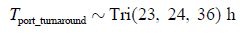
3.1.4 Operational parametersWe limit the design process to the fleet of cargo vessels, IBs, and port storage capacity. Consequently, all operational characteristics that are not directly dependent on these system components are considered as design parameters outside our field of influence. Given these boundaries of the design process, the main operational parameters are the port turn-around times and dry-docking times.
The port turn-around time include the total time for entering/leaving port, manoeuvring, mooring/unmooring, connection/disconnection of unloading arms, and loading/unloading. According to Tusiani and Shearer (2007) , for a large LNG tanker the aggregated time for these activities is typically around 24 h, out of which loading/unloading time is 12-16 h depending on the pump capacity. However, according to the same source, delays causing a turnaround time of up to 36 h are to be expected. Due to the occurrence of sea ice and the higher risk of extreme weather conditions and fog, we think that delays are more likely in the port of Sabetta than in the port of Zeebrugge. However, we do not have any data supporting this assumption. Thus, we assume that the turnaround time for all port calls corresponds to a triangular distribution given by Eq.(5).
|
|
(5) |

|
| Figure 3 Examples of calculated stochstic ice scenarios |
Existing rules and regulations require ships to be taken out of service for compulsory dry-docking once during a 5-year period. According to Moore Stephens (2013) , the average dry-docking time for a large tanker is around 20 days. Assuming 5-15 days of travel time to and from the dry-dock (starting from the port of Zeebrugge), we assume that the total down-time related to a dry-docking corresponds to a triangular distribution given by Eq.(6).
|
(6) |
As proposed by Erikstad and Ehlers (2014) , dry-dockings are scheduled for periods with little or no ice when the load on the transport system is at its minimum. In this manner, they will not cause a shortage in transport capacity.
3.1.5 Design constraintsDesign constraints determine boundaries of the design space. They consist of either physical limit values (bounds) determined in the form space, or of mandatory FRs determined in the function space. Various types of constraints include operational constraints determined by the transport task (e.g. maximum feasible ship size), technical constraints determined by the limits of technical feasibility (e.g. maximum feasible ship size), and regulatory constraints determined by rules and regulations. The main operational constraint of the present study concerns the vessel size. Due to limited water depth, we assume that the draught of the vessels need to be limited to around 12 m, and that the capacity of the vessels therefore needs to be limited to approx. 170 000 m3 (Minin, 2016). In terms of technical constraints, the ice-going capacity of a large ship is limited by technical feasibility but we are not able to specify a specific limit performance. However, based on Yamal LNG (2015) , we assume that it is feasible to build large LNG tanker with an ice-going capability of at least 2.1 m.
In terms of regulatory constraints, because the route goes through waters that are considered to be part of the exclusive economic zone of Russia, the ships must meet rules and regulations set by the Russian Federation. This means that they, in order to be permitted to operate year-round in all ice conditions on the South Kara Sea, must be constructed in accordance with the Russian ice class Arc7 (RS, 2015). For assisted operations, Arc6 is also accepted but results in an increased risk of damage in difficult ice conditions (RS, 2015).
Because the ships operate in what is defined as the Arctic by the IMO, they also must comply with the upcoming mandatory Polar Code. This means that the ships, in order to be permitted to operate year-round in thick first-year ice, must be constructed in accordance with the IACS Polar Class (PC) 4. In the present study, in order to make it possible to apply the goal/risk-based approach of the Polar Code, we assume that it is sufficient if the ships are acceptable in accordance with the Polar Code. In other words, we assume that if the ships are accepted in accordance with the Polar Code, they will also be accepted by the Russian Federation.
3.2 Concepts of operationsWhen searching for an AMTS solution, it is motivated to evaluate various concepts of operations (CONOPS), i.e. strategies for how to achieve the design objectives. In the present study, we consider the following CONOPS:
1) Use of independently operating ships with an ice-going capability of 2.1 m.
2) Use of ships with an ice-going capability of 1.4 m. Use of IB assistance when t > 1.2 m.
3) Use of ships with an ice-going capability of 1.4 m. Use of IB assistance when t > 0.5 m.
4) Use of ships with an ice-going capability of 1.4 m. Use of IB assistance when t > 0.5 m. Application of flexible contracting making it possible to deliver cargo to a more nearby destination (the port of Narvik) during years with exceptionally difficult ice conditions when the average speed along leg 3 is below 5 kn.
We start by determining a preliminary conceptual design for each CONOPS in terms of ship capacity, speed, and fleet size against a single set of design parameters. Because the cost efficiency of a ship generally increases by size, we determine that all ships are to have a capacity of 170 000 m3 corresponding to the assumed maximum feasible ship size.
In terms of speed, we determine that all ships must be able to maintain an open water speed of 19.5 kn considering increased resistance caused by heavy weather and fouling. In ice, the ships must perform in accordance with the determined CONOPS specific ice-going capability requirements, which is defined as the maximum heq in which a ship is able to maintain a continuous speed of 3 kn. With IB assistance, the ice-going capability is assumed to be 2.2 m. Assuming that the achievable speed is linearly dependent on heq, the speed requirements of the ships correspond thereby to the h-v curves presented in Fig. 4.
Because the concept of heq is based on averaging, it fails to consider the effect of large ridges exceeding the ridge penetration capability of the ships in question. Generally, ice ridges cause a resistance that is higher than a ship’s thrust forcing it to penetrate ridges using its inertia (Riska, 2010). The ridge penetration capability of a ship determines the maximum ridge size that a ship, for a given initial speed, can penetrate with one ram without losing all its kinetic energy. Generally, if a ship encounters a ridge exceeding its ridge penetration capability, the ship will get stopped. Once it has been stopped, it must try to reverse, build up speed, and ram into the ridge again. This ramming cycle is repeated until the ship manages to break through the ridge (Valkonen and Riska, 2014).

|
| Figure 4 Required speeds as a function of heq in light compressive ice |
In the present study, all ships are of type Double-Acting Tanker (DAT). An important advantage of DAT ships is that they can penetrate large ridges exceeding their ridge penetration capability at continuous speed without ramming (Forsén et al., 1998). This is achieved by using the ship’s azimuth thrusters to disintegrate the ridge by flushing (Niini et al., 2012). Based on Valkonen and Riska (2014) , we assume that the vessels are able to penetrate large ridges in this manner at a constant speed of around 0.5 kn. The corresponding speed pattern of the ship is presented in Fig. 5. It should be pointed out that in reality a ship would be able to penetrate a part of the large ridges using its inertia. Thus, the model presented in Fig. 5, in which the speed drops to 0.5 kn immediately as the ship encounter a large ridge, should result in a conservative estimate.

|
| Figure 5 Vessel speed in ridged ice |
The ridge penetration capability of a large ship can only be estimated reliably by model testing. Due to the lack of a more cost-efficient method, we assume that the ridge penetration capability of all our cargo ships is 18 m.
To account for the risk of compressive ice conditions, the ships need to have a power margin so that they are able to maintain the speed as determined by Fig. 4 in light compressive ice conditions. More difficult compressive ice conditions are assumed avoidable or short-lived, resulting in a marginal impact on the transit times of the ships.
The preliminary fleet size is determined in accordance with Tables 2-4. The assumed transit times represent 100-year worst (longest) transit times for each leg. During a round-trip, the vessels are assumed to experience an average delay of 6 h per port visit. The average waiting time for IB assistance is assumed to be 12 h.
The minimum average speed of 3 kn can be consider relatively high. However, if the we reduce the required speed so that the ice-going capability is defined in terms of the maximum heqin which the ships can maintain an average speed of for instance 2 kn, we find that for instance in the case of CONOPS 2, we need to increase the fleet size from 16 to 19 vessels in order to meet the transport task. Alternatively, the open water speed needs to be increased from 19.5 kn to 48 kn, which is not feasible. Thus, we conclude that in order to keep the required fleet size reasonable, the ice-going capability of the ships need to be defined as the maximum ice thickness in which the ships can maintain a speed of approx. 3 kn.
| CONOPS | Ship type | Ice class | Open water speed/kn | Ice-going capability, independent/m | Ice-going capability, assisted/m | for independent operation/m | Ridge penetration cap. /m |
| 1 | DAT | PC 4 | 19.5 | 2.1 | n/a | 2.1 | 18 |
| 2 | DAT | PC 4 | 19.5 | 1.4 | 2.2 | 2.1 | 18 |
| 3 | DAT | PC 4 | 19.5 | 1.4 | 2.2 | 0.5 | 18 |
| 4 | DAT | PC 4 | 19.5 | 1.4 | 2.2 | 0.5 | 18 |
| Leg | Distance/NM | heq/m | CONOPS 1 | CONOPS 2 | CONOPS 3 | CONOPS 4 | |||||||||
| Speed/kn | Transit time/d | Delay due to large ridges/d | Speed/kn | Transit time/d | Delay due to large ridges/d | Speed/kn | Transit time/d | Delay due to large ridges/d | Speed/kn | Transit time/d | Delay due to large ridges/d | ||||
| 1 | 1825 | 0 | 19.5 | 3.90 | 0.00 | 19.5 | 3.90 | 0.00 | 19.5 | 3.90 | 0.00 | 19.5 | 3.90 | 0.00 | |
| 2 | 203 | 1.70 | 6.0 | 1.42 | 0.02 | 6.3 | 1.34 | 0.00 | 6.3 | 1.34 | 0.00 | 6.3 | 1.34 | 0.00 | |
| 3 | 542 | 2.18 | 2.8 | 8.18 | 0.38 | 4.0 | 5.69 | 0.00 | 4.0 | 5.69 | 0.00 | 4.0 | 5.69 | 0.00 | |
| CONOPS | Total one-way sailing time/d | Port turnaround time/d | IB waiting time/d | Total round trip time/d | Number of vessels | Vessel cargo capacity/(×103m3) | Transport capacity/(103m3/d) |
| 1 | 13.50 | 1.25 | n/a | 29.5 | 18 | 170 | 103.8 |
| 2 | 10.93 | 1.25 | 1.0 | 26.4 | 16 | 170 | 103.2 |
| 3 | 10.93 | 1.25 | 1.0 | 26.4 | 16 | 170 | 103.2 |
| 4 | 8.55 | 1.25 | 1.0 | 21.6 | 13 | 170 | 102.3 |
In order to make the design task manageable, we divide each of the determined conceptual AMTS into a number of subsystems in accordance with Fig. 6. The various subsystems form three main subsystems: an operations (OPS) system, a safety, and an ENVP. In addition, they form two system levels: fleet and ship level.

|
| Figure 6 System division |
The fleet level OPS system consists of two or more ports and a fleet of cargo ships. On ship level, each cargo ship has a OPS system consisting of a buoyancy system, a propulsion system, and a cargo system. The buoyancy and propulsion system might be assisted by IBs. In addition to the OPS systems, each vessel has a ship level safety and ENVP system. The safety system consists of systems for hull protection, flooding mitigation, fire protection, ice protection, evacuation, and propulsion and steering unit protection. The systems for hull and propulsion and steering unit protection might be assisted by IBs, whereas the evacuation system might be supported by SAR units and emergency ports. The ship level ENVP systems consists primarily of an accidental discharge protection system, which might be assisted by external OSR units. IBs, SAR, an OSR units does not have to consists of units dedicated to one specific task. For instance, an IB might be able to act as a SAR and or OSR unit. Other commercial ships might act as SAR units as well. It is also possible for an icebreaking cargo ship to act as an IB for other cargo ship.
As described above, the ENVP and safety systems are all at ship level. As a result, each vessel must have a safety and a ENVP system that is independent of other ships. The OPS system, on the other hand, includes both fleet and ship level systems. This means that a single ship cannot perform its OPS function single handed because this requires among others loading and off-loading ports. On the other hand, it also means that an AMTS with multiple ships might be able to meet its transport task even though an individual vessel would be out of operation.
The design of a complete AMTS is an extensive task. Considering the objectives of the present study, we limit our attention to sub-systems (AMTS functions) meeting the following criteria: 1) We have access to methods and data enabling the application of the principles of GBD/RBD, 2) The design of the system is expected to be influenced by the choice of CONOPS.
Systems that at least partially meet these criteria include the fleet level OPS system, the hull protection system, and the propulsion system. The rest of the systems are not considered because they do not meet the determined criteria. The buoyancy system and the propulsion and steering unit protection system are not considered because of a lack of appropriate design methods enabling the application of GBD/RBD. The cargo system, the flooding mitigation system, the fire protection system, the icing protection system, the evacuation system, and the ENVP system are not considered because we assume that choice of CONOPS will not significantly affect their design. All systems that are not considered in the present study are assumed to be designed in accordance with established methods, rules, and regulations.
3.4 Subsystem design 3.4.1 In generalFor an efficient and purposeful design process, the various subsystems need to be designed in a specific order.
The first system to be designed is the fleet level OPS system. The function of the fleet level OPS system is to meet the transport task, i.e. to provide a transport capacity that meets the transport demand. The transport capacity depends on the number of cargo ships, as well as on the capacity and turnaround time of each ship. The turnaround time of a ship depends mainly on its speed (h-v curve), operating conditions (e.g. ice conditions), and port turnaround times. If a ship requires IB assistance, the transit times depends in addition on the waiting time for IB assistance and the convoy speed. The transport demand is considered absolute. However, port-based storage capacities provide a buffer against short-term shortages in transport capacity.
Once the fleet level OPS system has been designed, ship level OPS systems are to be designed to meet its performance requirements. In other words, the determined design variables of the fleet level OPS system act as performance requirements for the ship level OPS systems. For instance, the hull and propulsion system are to be designed to meet the assumed h-v curves of the ships. However, if it turns out to be infeasible or difficult to meet the determined performance requirements, the specifications of the fleet level OPS system need to be modified. In other words, the ship level OPS systems might determine performance limits or constraints for the fleet level OPS system.
The safety and the ENVP are enabling systems for the OPS system that must be adapted to its requirements. Thus, the safety and the ENVP systems are designed subsequently to the OPS system. However, when designing the OPS system, it is nevertheless necessary to foresee requirements (e.g. hull compartmentation) by the safety and ENVP systems.
3.4.2 Fleet level OPS systemThe design of the fleet level OPS system is carried out in accordance with Fig. 7 as follows. First, we determine design parameters, constraints, criteria and objective in accordance with section 3.1. The criterion is thereby to meet the transport demand in 100-year conditions, and the objective is to achieve a high level of cost-efficiency and robustness to variations in the operating conditions and financial parameters. Second, we determine a SimEvents (a discrete event simulation package within the MATLAB toolbox) Discrete Event Simulation (DES) model of the transport system. Third, for each CONOPS we determine four preliminary designs with different cargo storage capacities ranging 640 000 m3 to 1 120 000 m3. Initial preliminary fleet sizes as well as the speed and cargo carrying capacities of the ship are determined in accordance with Tables 2-4. Fourth, for each CONOPS and preliminary design, we iteratively determine the minimum fleet size meeting the design criteria. As a part of this process, we also determine the required number of IB to avoid prolonged waiting times for IB assistance. The performance of the various designs is assessed probabilistically in accordance with the Monte Carlo method. Specifically, we simulate their performances for 100 operating years, each characterized by a unique combination of design parameters values. Once we have determined the required fleet size for all CONOPS, a population of feasible designs is obtained. Sixth, among the population of feasible designs, we select the most promising design considering the objectives of the design process.

|
| Figure 7 Design process for determining the fleet level OPS system |
In DES, the behaviour of a system is modelled as an ordered sequence of events, each of which takes place at a specific point of time and results in a change in the state of the system (Craig, 1996). Because no change occurs between events, fast simulation of a complex AMTS operating over an extensive period of time is possible. In our DES model, which is presented in Fig. 8, individual vessels and cargo units are modelled as entities. A loaded ship is obtained by combining a ship entity with a specific number of cargo entities corresponding to the capacity of the ship entity. Ship entities are created at the start of the simulation and circulate thereafter in a closed loop until the simulation stops. Cargo entities are produced at a fixed rate and leave the system once they have been transported to their destination. During the simulation, the ship and cargo entities are stopped for various lengths of time corresponding to the duration of events such as completing a specific leg, visiting a port, and waiting for IB assistance.

|
| Figure 8 Overview of the applied SimEvents simulation model |
The model can be thought of as consisting of nine sub-models:
1) A fleet initialisation module that produces a specific number of cargo ships at the start of the simulation.
2) A LNG production and storage unit. LNG is continuously produced at a fixed rate. Produced LNG is stored until it is loaded onto a ship.
3) The port of Sabetta. New and returning ships are loaded with cargo. The port can serve two ships at a time. If both berths are occupied, incoming ships wait until a berth becomes available. If at least one full shipload of cargo is waiting for transport when the ship arrives, the total port turnaround time is assumed to correspond to the distribution given by Eq.(5). Otherwise, the ship must first wait until a full shipload has been produced.
4) The sailing distance Sabetta-Zeebrugge. The total sailing time is calculated as the cumulated sailing time for the three legs plus possible waiting time for IB support.
5) The port of Zeebrugge. We assume that the LNG terminal makes maximum two berths available for our ships. If both berths are occupied, the incoming ships need to wait for an available berth. Once a berth becomes available, the total port turnaround time is assumed to correspond to the distribution given by Eq.(5).
6) The LNG market. Unloaded LNG is absorbed by the LNG market.
7) The sailing distance Zeebrugge- Sabetta is modelled in the same manner as the distance Sabetta-Zeebrugge/Narvik.
8) IBs. One IB assists one cargo ship at a time. Once the assistance is over, the IB is available to assist other ships.
9) A dry-dock. Dry-dockings are simulated by taking ships out of operation for a time corresponding to the total down-time required for the operation.
The determined population of feasible design with regards to fleet size and cargo storage capacity are presented in Fig. 9. As seen in the figure, the required fleet size is strongly dependent on the cargo storage capacity. By increasing the cargo storage by 75% from 640 000 m3 to 1 120 000 m3, the fleet size can be reduced by 1-2 ships depending on the CONOPS.

|
| Figure 9 Feasible designs with regard to fleet size and cargo storage capacity |
Because we are lacking data on the costs of LNG storages, we are unable to determine precisely what combination of fleet size and cargo storage capacity results in the highest level of cost-efficiency. To keep the costs of the carious CONOPS comparable, we select a cargo storage of 800 000 m3 for all CONOPS. The corresponding required number of ships are summarized in Table 5.
Our determined storage capacity of our cargo storage is thereby 160 000 m3 or 25% or larger than the storage of our reference system (Yamal LNG, 2015). We decided for the larger storage capacity based on the assumption that the savings obtained by reducing the fleet size by one ship exceed the added costs for the increased storage capacity.
| CONOPS | Number of ships | Cargo capacity per ship/m3 |
| 1 | 15 | 170 000 |
| 2 | 14 | 170 000 |
| 3 | 14 | 170 000 |
| 4 | 13 | 170 000 |
If we reduce each fleet size presented in Table 5 by one ship, each CONOPS fails to meet the transport demand at least once during 100 simulate years. The number of failures as well as the consequences of each failure are presented in Fig. 10. For CONOPS 1 there is a 1% risk of losing up to 200 000 m3, for CONOPS 2 there is a 3% risk of losing up to 380 000 m3, for CONOPS 3 there is a 2% risk of losing up to 240 000 m3, and for CONOPS 4 there is a 9% risk of losing up to 270 000 m3. In all cases, the losses could be avoided by increasing the cargo storage capacity by a volume approximately corresponding to the maximum volume of lost production. In this manner, the storage capacity could be adapted to each CONOPS separately.

|
| Figure 10 The maximum number of ships resulting in an operational reliability that is below 100% for a cargo storage capacity of 800 000 m3 |
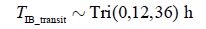
IBs are modelled as resources that assist one vessel at a time. A ship in need of assistance waits until there is an available IB. However, the simulation model is not able to determine the time it takes for an available IB to reach a ship in need of assistance. Therefore, this transit time is determined in accordance with Eq.(7).
|
(7) |
In the simulation model, the total waiting time depends thereby both on the number of IBs and the transit time determined based on Eq.(7). As shown in Fig. 11, a total of 7 IBs is required to avoid the risk of prolonged waiting times. It should be pointed out that the existing fleet of IBs is insufficient to meet this demand.

|
| Figure 11 IB waiting time for various number of IBs |
The function of a ship’s propulsion system is to provide the level of thrust required by the ship to perform in accordance with the h-v curves determined in Fig. 4. In order to determine the required level of thrust, the open water and ice resistance of the ship must first be estimated. However, because there is no cost-efficient and accurate method for the determination of a ship’s ice resistance, we are not able to estimate the required level of thrust and consequently we are also not able to estimate the required level of propulsion power. Therefore, we estimate the required propulsion power based on a reference ship. As reference ship we chose the “Yamalmax” ship type as defined by Yamal LNG (2015) and Wärtsilä(2014), which has a LNG capacity of 172 600 m3, an ice-going capability of 2.1 m, and a propulsion power of roughly 65 000 kW. Because the specification of the CONOPS 1 vessels corresponds to those of of the reference ship, we assume that their power requirementis the same, i.e. 65 000 kW. In order to determine the power requirement of the vessels of CONOPS 2-4, we assume as a simplification roughly based Lee (2008) that the power requirement and the ice-going capability are proportional. Based on this assumption, we determine the power requirements for the CONOPS 2-4 ships in accordance with Eq.(8).

|
(8) |
The power demand of 43 000 kW determined for the CONOPS 2-4 vessels can be compared with the power demand of 41 250 kW of MS Valencia Knutsen, which is a LNG carrier with a capacity of 173 400 m3, an open water speed onf 19.5 kn, and an ice class of 1 A (Knutsen, 2016). We assume that the slightly higher power demand of our CONOPS 2-4 vessels is due to their higher ice class.
The CONOPS 1 ships are assumed to use their full power only when operating in ice. When operating in open water, their power requirement is assumed to be 45 000 kW. The ships of CONOPS 2-4 are assumed to continuously operate at their full power of 43 000 kW.

|
| Figure 12 Simulated ice exposures (FYI=first-year ice) |
The function of the hull protection system is to protect the hull from structural loads, primarily ice induced loads. Hull protection can be achieved either by reducing the loads that the hull is subjected to (e.g. by IB assistance), or by making the hull more resistant towards loads (e.g. by ice-strengthening). The design of the hull protection system is strictly regulated by existing rules and regulations. Specifically, the system must meet regulations set by the upcoming Polar Code and the Russian Federation. However, in the present study, we assume that it is sufficient if the vessels are acceptable in accordance with the Polar Code, which requires that the ships, in order to be permitted to operate in thick (>120 cm) first-year ice, must be constructed in accordance with the IACS Polar Class (PC) 4 (IMO, 2016).
A major weakness of the polar class regulations is that they make no difference between independent and assisted operation. In addition, they do not consider the actual ice exposure (e.g. for how many hours per year the ships operate in thick first-year ice). In the present study, we aim to address these weaknesses by applying a probabilistic design method developed by Jordaan et al.(1993) and later on applied on ships operating on the Northern Sea Route (NSR) by Tõns et al.(2015) . The method makes it possible to determine the probabilistic extreme loads based on a ship’s ice exposure determined in terms of the average time and speed a ship operates in various ice conditions. The ice conditions are classified as easy, medium, and heavy natural or brash ice based on the prevailing level ice thickness in accordance with Table 6.
| Easy ice conditions | Medium ice conditions | Heavy ice conditions |
| ≤ 0.7 | ≤ 1.2 | > 1.2 |
For the determination of the ice exposure, we apply the DES model described in Section 3.4. Specifically, we run the simulation for 100 years and monitor and document the ice exposure of each vessel. Once the simulation is finished, we determine the annual average ice exposure per vessel for each simulated year. The simulation outcome, which is presented in Fig. 12, indicate that the ice exposure varies significantly from year to year. For instance, in the case of CONOPS 1, the annual exposure to thick first-year ice varies between 0 hr and 1 100 h. As expected, the exposure also strongly depends on the chosen CONOPS. For instance, in the case of CONOPS 3, in which the vessels receive IB assistance when t > 0.5 m, the exposure to medium and thick natural ice is zero.

|
| Figure 13 100-year extreme loads for various CONOPS |
Based on the determined ice exposure and the method presented by Tõns et al.(2015) , the 100-year extreme ice structural loads is calculated as a function of the design area in accordance with Fig. 13. As shown by the figure, the obtained load curves are quite similar for the various CONOPS:s, i.e. the use of IB assistance does not appear to significantly affect the extreme loads. This means that the required level of ice-strengthening is similar for all ships. Fig. 13 also shows the design loads of the various PC classes. In accordance with Taylor et al.(2009) , the minimum design area of interest is typically around 0.6 m2. If we focus on a typical design area within the range 0.6-1 m2, we find that the extreme loads are below the design load of PC 3. This indicates that the prescribed PC 4 standard is appropriate for all our ships. However, it should be pointed out that additional response analysis is required to enable a more precise comparison between the calculated loads and the PC design loads. The determined extreme loads could for instance be used as input for direct analyses (e.g. finite element method analyses) to for instance verify that a PC 4 ship is strong enough.
It should also be pointed out that both the rule-based and the probabilistic methods use the concept of a uniform pressure patch to apply the design load, therefore not directly accounting for the effects of spatial variations found in ice load measurements. Erceg et al.(2014) analysed medium-scale ice pressure indentation experiments using measured load pattern, concluding that the uniform application of the design pressure can result in non-conservative structural designs. Alternatively, they proposed a Simplified Non-uniform Pressure Patch (SNPP) to serve as an alternative to the rule-based ice load application model. Early approach of SNPP was presented in Ehlers and Kujala (2013) and Ehlers et al.(2014) .
3.5 Probabilistic performance assessment 3.5.1 Design specific financial parametersFor the comparison of the cost-effectiveness of competing design alternatives, we determine three types of financial parameters: daily time charter rate (including capital, crew, and maintenance costs), fuel price, and IB tariffs.
The daily time charter rate of an arctic cargo ship depends on factors such as cargo carrying capacity, ice-going capability, and ice class. Historically the time charter market has been highly volatile as the rates are strongly dependent on the prevailing freight rates (Stopford, 1997). In this study we assume that the daily time charter rates are fixed by long-term charter contracts in accordance with Table 7. In order to account for additional costs related to the higher ice-going capability of the CONOPS 1 vessels, their daily time charter rate is assumed to be 5% higher than the rate of the vessels of CONOPS 2-5.
| Design | Daily time charter rate (USD/d) |
| CONOPS 1 | 130 000 |
| CONOPS 2-4 | 123 500 |
Naturally, the fuel price depends on what type of fuel is used. Traditionally, deep-sea shipping, arctic shipping included, operates on on Heavy Fuel Oil (HFO) (Nilsen, 2014). However, the present route goes through the North Sea, which is an Emission Control Area (ECA) where the maximum allowed Sulphur emissions is limited to 0.1% (IMO, 2014). In order to comply with this regulation, ships are in practice required to operate either on Marine Diesel Oil (MDO) or Marine Gas Oil (MGO), or to apply an exhaust cleaning system such as a scrubber. In the future, the ECA area might be expanded to include the sea areas off the Norwegian coast (Exxon Mobile, 2015). Thus, for the case of simplicity, we assume that our ships operate continuously on MDO.
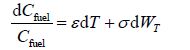
For the modelling of future MDO prices, we apply a stochastic process known as Geometric Brownian Motion (GBM), which is commonly used within finance for the prediction of future non-negative asset prices. The fuel price Cfuel is said to follow a GBM if it satisfies the stochastic differential equation given by Eq.(9).
|
(9) |
where is the volatility of Cfuel, ε is the drift of Cfuel, dT is the time increment, and WT is a Wiener process/Brownian motion (Rehn, 2015).
The operation is assumed to start 01.08.2019 and to last for 25 years, i.e. until 31.07.2043. In order to create four different fuel price scenarios (very high, high, medium, and low) for this period, we determine four different sets of input parameter in accordance with Table 8. The start price is determined based on Bunkerindex (2016) . The resulting price scenarios, which were determined using a GBM function determined by Rehn (2015) , are presented in Fig. 14.
| Scenario | Start price/ (USD/MT) | Drift /% | Volatility σ/% |
| Very high price | 350 | 3.0 | 5 |
| High price | 350 | 1.5 | 5 |
| Medium price | 350 | 0 | 5 |
| Low price | 350 | −3.0 | 5 |

|
| Figure 14 Determined MDO price scenarios |
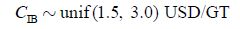
In the NSR area, costs for IB assistance are calculated based on the assisted vessel’s Gross Tonnage (GT), ice class, and the number of zones through which the ship is assisted (CHNL, 2015). According to CHNL (2015) , the maximum IB tariff for a 110 000 GT Arc7 vessel that is assisted within one zone (South Kara Sea) is RUB 14.5 million or around USD 184 000 (USD/RUB=78.47). This corresponds to around 1.67 USD/GT. However, the tariff is subject to uncertainty (Gritsenko and Kiiski, 2015). Thus, in the present study we assume that the IB tariffs per assisted voyage are determined in accordance with Eq.(10).
|
(10) |
In order to choose the most promising design, a probabilistic performance assessment is carried out using the Monte Carlo method. Specifically, for each CONOPS we simulate the time charter costs, fuel costs, and IB costs for 4×25-year periods representing various fuel price scenarios. The objective is to determine which CONOPS results in the lowest average costs. In addition, we want to quantify the robustness of the various CONOPS in terms of the variance of the average annual costs per transported cargo unit.
For each simulated year, the time charter costs, fuel costs, and IB costs are determined in accordance with the following. Time charter costs are calculated as the product of the number of ships, the daily time charter rate per ship, and the total operating time (all time except off-time due to dry-docking). For each CONOPS, the number of ships is determined in accordance with Table 5 and the daily time charter rates are determined in accordance with Table 7. Fuel costs are determined based on the cumulated number of operating hours at various operating modes (open water, independent operation in ice, and assisted operation in ice), the power requirement at each operating mode, and the Specific Fuel Consumption (SFC). The operating hours are determined by using the simulation model presented in section 3.4.2, the power requirements are as determined in section 3.4.3, and the SFC is assumed to be 170 g/ (k·W·h) for all ships. IB costs are calculated based on the number of assisted voyages, the vessel gross tonnage, and the IB tariff. The number of assisted voyages are determined using the simulation model presented in section 3.4.2. Based on the reference ship Valencia Knutsen (Knutsen, 2016), the GT value of all ships is assumed 110 000 m3. The IB tariff is determined as a random number drawn from the distribution determined by Eq.(10).
3.5.3 ResultsThe outcome of the performance assessment, which is presented in Fig. 15, indicate that CONOPS 4 provides the lowest costs average at 23 USD per transported cubic meter of LNG. However, in CONOPS 4 up to 0.6% of the cargo volume is transported to the more nearby port of Narvik (Norway) instead of the port of Zeebrugge. Thus, in terms of costs, CONOPS 4 is not directly comparable with CONOPS 1-3. Among the directly comparable CONOPS 1-3, CONOPS 2-3 are the most cost efficient at an average of 24 USD/m3. CONOPS 1 is around 8% costlier at an average of 26 USD/m3. In terms of robustness, the results indicate that CONOPS 3-4 are the most robust with a variance of 14, CONOPS 2 is the second most robust with a variance of 16, and CONOPS 1 is the least robust with a variance of 20. This ranking is explained by the fact that independent operation results in a higher fuel consumption resulting in a higher exposure to variations in fuel prices.

|
| Figure 15 Probabilistic performance assessment |
The results indicate thereby that CONOPS 3 provides the best overall performance among the directly comparable CONOPS and that IB assistance favours both cost-efficiency and operational robustness. The relatively small gain provided by CONOPS 4 in terms of cost efficiency does probably not compensate for the penalty related to the flexible contracting. However, it should be pointed out that CONOPS 1 is the only feasible solution for the existing fleet of IBs.
3.6 Final designBased on the above presented design process, we chose a fleet consisting of 14 ships, each with a cargo capacity of 170 000 m3, an ice-going capability of 1.4 m, and an ice class of Arc7. In order to maintain a sufficient transport capacity, the ships require IB assistance when heq exceeds 0.7 m. In addition, in order to allow for a temporary reduction in transport capacity during periods of difficult ice conditions, a port-based storage of 800 000 m3 is required. In comparison with the reference design presented by Yamal LNG (2015) , we have thereby reduced the fleet size by 12.5% from 16 to 14 ships, and reduced the ice-going capability of the ships by 33% from 2.1 m to 1.4 m. On the downside, we have increased the required port-based storage capacity by 25% from 640 000 to 800 000 m3, as well as made the fleet dependent on IB assistance. Due to the large size of the fleet, we estimate that in total 7 IB are required to avoid prolonged waiting times for IB support. We estimate that, in order to meet this IB demand, it would be necessary to extend the existing fleet of IBs.
4 DiscussionThe outcome of the case study demonstrates the amount of information that can be obtained by incorporating simulations and probabilistic design parameters into the design process. If we let Tables 2-4 represent a case of deterministic design, the value of the obtained information becomes apparent. Based on the tables it is for instance not possible to estimate the IB and fuel costs of the various CONOPS and consequently also not possible to determine which CONOPS provides the highest level of cost-efficiency. Anyhow, assuming that we would have selected CONOPS 3, we would conclude that we need a fleet of 16 vessels to obtain the required level of transport capacity in worst expected operating conditions. We could have argued that this represents a conservative design because the buffer provided by the port-based storage capacity is not considered. Based on SBD, on the other hand, we were able to demonstrated that a fleet of 14 ships is sufficient to meet the design objective. Obviously, given the high daily time charter costs of the ships, the avoidance of redundant ships is very important.
The assessment of the cost-efficiency of the various CONOPS indicates clearly that the use of IB assistance increases cost-efficiency. In order to understand why this is the case, we analyse the division of time between operation in open water, independent operation in ice, and assisted operation in ice. The results of the analysis, which are shown in Fig. 16, indicate that in the case of CONOPS 1, the vessels operate on average just 54 days per year or 15% of the time in ice. The CONOPS 1 vessels only benefit from their superior ice-going while operating in ice. Apparently, in the present case, the savings obtained by not having to pay IB tariffs were not large enough to compensate for the added daily time charter and fuel costs from which the CONOPS 1 ships suffer during all other time, i.e. 85% of the time.

|
| Figure 16 Operating times at various operating modes |
In accordance with Fig. 15, there are significant annual variations in the costs per transported cargo unit. Obviously, the variations are due to both variations the ice conditions, and due to variations in the fuel prices and IB tariffs. In order to isolate the effect of variations in the ice conditions, we calculated the annual operating costs for 100 years for a fixed fuel price (USD 500/MT) and IB fee (USD 2/GT). The outcome of the calculations, which are presented in Fig. 17, shows that for a fixed fuel price and IB tariff, annual variations in costs are quite marginal. This indicates that variation in costs are primarily driven by variations in the fuel price and IB tariff.

|
| Figure 17 Costs with fixed fuel price and IB tariff |
Modelling of ice conditions is a complex and challenging task. Because future ice conditions will always be uncertain, there is not one correct model and the accuracy of any model can only be assessed in retrospect. In the present paper we chose to model the ice conditions based on historical ice data assuming that the future climate and consequently also the ice conditions will remain statistically unchanged. An alternative approach is to determine future ice scenarios using a climate model predicting the development of the climate and consequently also the ice conditions (e.g. warming climate and consequently diminishing ice conditions). This approach has been applied in multiple studies. For instance, Stephenson et al.(2013) present a study in which future sea ice scenarios were determined based on numerical sea ice model referred to as the Los Alamos Sea Ice Model (CICE). Another example is Bergström et al.(2014) , in which a case study was carried out using ice data produced by a numerical climate model referred to as SINMOD (SINTEF, 2015). In accordance with the study, the SINMOD model predicts realistic ice coverage values but has a tendency to predict unrealistically high ice thicknesses.
The applied historic temperature and ice data provided by Romanov (1995) and Riska (1995) originates primarily from the 1970s and the 1980s and can therefore rightly be considered old. Despite significant effort, we were not able to find a complete set of newer data based on which it would have been possible to calculate month and area specific average level ice thicknesses. There is not a lack of ice data in itself, but the available newer data is generally presented in terms of ice charts that determines ice thicknesses in terms of thickness ranges (e.g. 70-120 cm) that we consider too wide for the determination of relevant month and area specific ice thickness distributions. Anyhow, we did find some newer sources providing information about the annual peak ice conditions along the route. For instanceRosneft (2016) states that the annual maximum level ice thickness in the Kara Sea ranges between 1.2 m and 1.6 m, Johannessen et al.(2007) states that the level ice thickness in the south Kara Sea ranges between 1.5 m and 1.6 m on average, and Østreng (1999) states that average annual maximum level ice thickness in the Peachora Sea and in the South Kara Sea are 1.0 m and 1.3 m respectively. The figures by Østreng (1999) agree quite well with our applied average values of 1.1 m for the Pechora Sea and 1.4 m for the South Kara Sea.
The ratio between the average level ice thickness and its standard deviation as well as the distributions based on which various ice ridging characteristics (e.g. sail height and keel draft) were determined originates largely from the same sources as the level ice data (e.g. Romanov, 1995). However, in contrary to the ice thickness and concentration values, these ratios should not be affected by changes in the average ice conditions.
In order to increase the fidelity of the ice model, in particular month and area specific ice ridge density distributions are sought after. In the present study we assume that the same ridge density distribution applies for the whole route. In addition, we assume that the ridge density remains constant along each sub-leg during one ice-year. Naturally, these are rough simplifications as the ridge density distribution is known to be area specific and the ridge density typically increases towards the spring.
5 ConclusionsBased on the outcome of the case study, we can now answer the research questions presented in chapter 1. In response to the first research question, we conclude that valuable additional information can be obtained by applying simulations and probabilistic design parameters in the design process. Monte Carlo simulation makes it possible to determine the average (expected) performance of a system depending on multiple unrelated uncertain parameters. This will likely result in a less conservative solution than if the system is designed against a set of deterministic parameter values representing the “worst expected” operating conditions. In addition, the combined utilization of simulations and probabilistic design parameters makes it possible to determine the long-term ice exposure based on which an appropriate level of ice-strengthening can be determined. Furthermore, the use of simulation makes it possible to access various interaction (e.g. queuing time for available port berths) as well as various self-enforcing (e.g. the waiting time for IBs increases as the ice-conditions get worse) effects. In response to the second research question, we conclude that significant advantages can be obtained by system thinking including the following. First, the consideration of the whole transport system enables a systematic comparison of the merits of various CONOPS. Second, especially in the case of industrial shipping, it makes it possible to consider the effect of port-based cargo storage facilities allowing temporary shortages in the transport capacity. Third, it makes it possible to consider the benefits of a large fleet: a transport system with a large fleet is less sensitive towards disturbances affecting individual ships.
The study did not consider the effect of long term development trends in terms of ice conditions. Several studies indicate that the volume and extent of sea in the arctic is decreasing. However, we were not able to incorporate this forecast into our ice scenario model based on historical data. Another factor that we did not consider is the utilization of surplus transport capacity for other transport tasks. In our study, surplus transport capacity resulted only in added time charter costs. However, in the summer months it could for instance be used for shipments to Asia along the NSR. Also, a surplus transport capacity would allow slow steaming, reducing the fuel costs and thus also the penalty of overcapacity.
The case study highlights several gaps in the available design methods and tools. In terms of ship performance prediction, there is for instance a lack of cost-efficient, reliable, and fast methods for the determination of the ice resistance and the ridge penetration capability of large ships. In terms of ice loads, there is a lack of a precise method for relating the estimated physical ice loads to the PC rules. The study also highlights gaps in the available input data. In particular, there is lack of ice data on transitional ice conditions. Because the available ice data generally relate to the annual worst ice conditions, there is little or no data on how for instance the ridge density develops throughout the cold period. In addition, there is a complete lack of data based on which to determine the likelihood and magnitude of compressive ice. Thus, it must be underlined that the model rests on strong simplifications and that its usefulness rest rather on stochastic performance assessment rather than on a predictive value.
To sum up, the outcome of the present case study indicates that SBD enables better informed design decisions compared to using conventional design methods in which a AMTS is designed against a set of deterministic design criteria. However, in order to increase the applicability of the method, significant gaps in the available tools, methods, and data need to be addressed.
List of abbreviaitonsAMTS Arctic maritime transport system
IB Icebreaker
CONOPS Concepts of operations
DAT Double-acting tanker
DES Discrete event simulation
ECA Emission control area
ENVP Environmental protection
FYI First-year ice
GBM Geometric Brownian motion
GBD Goal-based design
GT Gross tonnage
HFO Heavy fuel oil
h Hours
IACS International association of classification societies
kn Knots
LNG Liquefied natural gas
MDO Marine diesel oil
MGO Marine gas oil
MT Metric ton
NM Nautical miles
NSR Northern sea route
OPS Operations
OSR Oil spill response
PC Polar class
RBD Risk-based design
SAR Search and rescue
SBD Simulation-based design
SFC Specific fuel consumption
SNPP Simplified non-uniform pressure patch
USD United states dollar
List of symbolsC Price/Tariff
c Ice coverage
dfd Freezing degree days
heq Equivalent ice thickness
hr Ridge keel draft
hr_avg Average ice ridge keel draft
hs Ridge sail height
hs_avg Average ridge sail height
I Ice condition severity index
P Power
T Time/Duration
t Level ice thickness
v Speed
wr Ridge width
WT Wiener process/Brownian motion
α Ice ridge shape factor
ε Drift (time series)
μ Mean value
ρ Ice ridge density
σ Standard deviation / volatility
λ Distribution shape parameters (for ice ridge keel draft)
| AARI, 2015. Review ice charts for the Arctic Ocean. Russian Arctic and Antarctic Research Institute. [2016-04-25]. http://www.aari.ru/projects/ecimo/ |
| Bauch HA, Pavlidis YA, Polyakova YI, Matishov GG, Kog N, 1999. Peachora Sea environments: past present, and future. Ber. Polarforsch. Meeresforsch. 501 (2005). |
| Bergström M, Ehlers S, Erikstad SO, Erceg S, Bambulyak A, 2014. Development of an approach towards mission-based design of arctic maritime transport systems. Proc. 33th International Conference on Ocean, Offshore and Arctic Engineering, San Francisco, OMAE2014-23848. |
| Bunkerindex, 2016. Bunker index MDO. [2016-03-15]. http://www.bunkerindex.com/prices/bixfree_1512.php?priceindex_id=4 |
| Centre for High North Logistics (CHNL), 2015. Admittance criteria and icebreaker tariffs. [2016-03-10]. http://www.arctic-lio.com/nsr_tariffsystem |
| Craig D, 1996. Discrete-Event simulation. Memorial University of Newfoundland. [2015-12-15]. http://www.cs.mun.ca/~donald/msc/node11.html |
| Ehlers S, Erceg B, Jordaan IJ, Taylor R, 2014. Structural analysis under ice loads for ships operating in Arctic waters. Proceedings of MARTECH 2014, 2nd International Conference on Maritime Technology and Engineering, Lisbon, 449-454. |
| Ehlers S, Kujala P, 2013. Cost optimization for ice-loaded structures. In Analysis and Design of Marine Structures. Taylor & Francis Group, London, 111-118. DOI: 10.1201/b15120-18 |
| Erceg B, Taylor R, Ehlers S, Leira BJ, 2014. A response comparison of a stiffened panel subjected to rule-based and measured ice loads. Proceeding of the 33rd International Conference on Ocean, Offshore and Arctic Engineering, Volume 10: Polar and Arctic Science and Technology, San Francisco, OMAE2014-23874. |
| Eriksson P, Haapala J, Heiler I, Leisti H, Riska K, Vainio J, 2009. Ships in compressive ice: Description and operative forecasting of compression in an ice field. Research report No. 59, Finnish Maritime Administration. |
| Erikstad SO, Ehlers S, 2014. Simulation-based analysis of arctic LNG transport capacity, cost and system integrity. Proc. 33th International Conference on Ocean, Offshore and Arctic Engineering, San Francisco, OMAE2014-24043. DOI: 10.1115/OMAE2014-24043 |
| Exxon Mobile, 2015. Preparing for change in emission controlled areas by 2015. [2016-01-15]. https://www.xxonmobil.com/MarineLubes-En/your-industry_hot-topics_emission-control-area-2015.aspx |
| Forsén AC, Kivelä J, Ranki E, 1998. The NSR simulation study work package 4: Design of the NSR service ships. INSORP Working Paper No. 120-1998. |
| Gritsenko D, Kiiski T, 2015. A review of Russian ice-breaking tariff policy on the northern sea route 1991–2014. Polar Record, 52(2), 144-158. DOI: 10.1017/S0032247415000479 |
| Hagen A, Grimstad A, 2010. The extension of system boundaries in ship design. International Journal of Maritime Engineering, 152, A-17-A-28. DOI: 10.3940/rina.ijme.2010.a1.167 |
| Heideman T, Salmi P, Uuskallio A, Wilkman G, 1996. Full-scale ice trials in ridges with the Azipod (Azimuthing PoddedDrive) Tanker Lunni in the Bay of Bothnia in 1996. Proceedings of the Polartech 96 International Conference on Development and Commercial Utilization of Technologies in Polar Regions. |
| IMO, 2014. Ships face lower sulphur fuel requirements in emission control areas from 1 January 2015. [2015-11-15]. http://www.imo.org/en/MediaCentre/PressBriefings/Pages/44-ECA-sulphur.aspx#.Vr3eeby9jzI |
| IMO, 2016. International code for ships operating in polar waters (POLAR CODE). MEPC 68/21/Add.1. Annex 10. [2015-11-15]. http://www.imo.org/en/MediaCentre/HotTopics/polar/Documents/POLAR%20CODE%20TEXT%20AS%20ADOPTED.pdf |
| ISSC, 2015. Arctic technology. International Ship and offshore Structures Congress (ISSC), Committee V.6 report. |
| ISO, 2010. Petroleum and natural gas industries - Arctic offshore structures. ISO 19906: 2010. |
| Jordaan IJ, Maes MA, Brown PW, Hermans IP, 1993. Probabilistic analysis of local ice pressures. Journal of Offshore Mechanics and Arctic Engineering, 115, 83–89. DOI:10.1115/1.2920096 |
| Johannessen OM, Alexandrov V, Frolov IY, Sandven S, Pettersson LH, Bobylev LP, Kloster K, Smirnov VG, Mironov YU, Babich NG, 2007. Remote sensing of sea ice in the Northern Sea Route: Studies and applications. Springer Praxis, Chichester, 50. |
| Knutsen, 2016. Valencia Knutsen. Knutsen OAS Shipping AS. [2016-01-20]. http://knutsenoas.com/shipping/lng-carriers/valencia/ |
| Lee SK, 2008. Combining ice-class rules with direct calculations for design of arctic LNG vessel propulsion. ABS technical papers 2008, American Bureau of Shipping, 17–35. |
| Leppäranta M, 2011. The drift of sea ice. Second edition, Springer-Praxis, Heidelberg, Berlin. |
| Minin M, 2016. Construction of Sabetta seaport will require unique technologies. Arctic-info. [2016-01-15]. http://www.arctic-info.com/ExpertOpinion/15-07-2013/construction-of-sabetta-seaport-will-require-unique-technologies |
| Moore Stephens, 2013. OpCost 2013. Moore Stephens Consulting Ltd. |
| Niini M, Arpiainen M, Mattsson T, 2012. Aurora slim polar research icebreaker. Proceedings of the Arctic Technology Conference, Houston, OTC 23772. |
| Nilsen, T, 2014. Debate on Arctic shipping heats up. Barents Observer. [2015-11-15]. http://barentsobserver.com/en/arctic/2014/01/debate-arctic-shipping-heats-20-01 |
| Papanikolaou A, 2009. Risk-based ship design-methods, tools and applications. Springer, Berlin-Heidelberg, 10–13. |
| Rehn CF, 2015. Identification and valuation of flexibility in marine systems design. Master thesis, Norwegian University of Science and Technology, Trondheim, 29–30. |
| Riska K, 1995. Ice conditions along the north-east passage in view of ship trafficability studies. Proc. 5th International Offshore and Polar Engineering Conference, The Hague, Netherlands(II), 420–427. |
| Riska K, 2009. Definition of the new ice class IA Super +. Research Report No. 60. Winter Navigation Research Board. Finnish Maritime Administration. |
| Riska K, 2010. Ship-ice interaction in ship design: theory and practice. Course Material, NTNU. http://www.eolss.net/ sample-chapters/c05/E6-178-44-00.pdf |
| Romanov IP, 1995. Atlas of ice and snow of the Arctic Basin and Siberian Shelf Seas. Backbone Publishing Company. |
| Rosneft, 2016. Russia’s Arctic Seas. [2016-05-13]. http://www.rosneft.com/Upstream/Exploration/arctic_seas/ |
| RS, 2015. Rules for the classification and construction of sea-going ships. Russian Maritime Register of Shipping, Vol. 1. |
| Schartmüller B, Milakovic AS, Bergström M, Ehlers S, 2015. A simulation-based decision support tool for Arctic transit transport. Proceedings of the ASME 2015 34th International Conference on Ocean, Offshore and Arctic Engineering, St. John's, Canada. |
| SINTEF, 2015. SINMOD - A physical - chemical -biological model system. [2016-05-12]. http://www.sinmod.no/images/ |
| Stephenson SR, Laurence CS, Brigham LW, Agnew JA, 2013. Projected 21st-century changes to Arctic marine access. Climate Change, 118(3), 885–899. DOI:10.1007/s10584-012-0685-0 |
| Stopford M, 1997. Marine economics. London: Routledge. |
| Taylor RS, Jordaan IJ, Li L, Sudom D, 2009. Local design pressures for structures in ice: analysis of full-scale data. Proceedings of the ASME 2009, 28th International Conference on Ocean, Offshore and Arctic Engineering, Honolulu, 61-69. DOI: 10.1115/OMAE2009-79386 |
| Tõns T, Freeman R, Ehlers S, Jordaan IJ, 2015. Probabilistic design load method for the Northen Sea Route. Proceedings of the ASME 2015, 34th International Conference on Ocean, Offshore and Arctic Engineering, St. John’s, Canada. DOI: 10.1115/OMAE2015-41841 |
| Tusiani MD, Shearer G, 2007. LNG: a nontechnical guide. PennWell Books. |
| Valkonen J, Riska K, 2014. Assessment of the feasibility of the arctic sea transportation by using ship transit simulation. Proc. 33th International Conference on Ocean, Offshore and Arctic Engineering, San Francisco, California, USA, V010T07A045. DOI: 10.1115/OMAE2014-24188 |
| Wärtsilä, 2014. Wärtsilä dual fuel engines chosen to power Arc 7 design icebreaking LNG carriers. Press release. [15, 2015-12-15]. http://www.wartsila.com/media/news/10-11-2014-wartsila-dual-fuel-engines-chosen-to-power-arc-7-design-icebreaking-lng-carriers |
| Yamal LNG, 2015. About Yamal LNG. [2016-12-15]. http://yamallng.ru |
| Østreng W, 1999. The natural and societal challenges of the Northern Sea Route: A reference work. Springer-Science+ Business Media.B.V, 117, 248. |