


 ,
,
2. Khalifa University of Science, Technology and Research, P.O. Box 127788, Abu Dhabi, UAE
1 Introduction
Ethylene, which is also known as ethene, is a colorless flammable chemical substance produced on an industrial scale by steam-cracking hydrocarbons. It is widely used in the chemical industry to produce substances such as polyethylene, ethylene dichloride, ethanol, glycols, and styrene is also used as a coolant and fuel for cutting and welding metals. It is also considered to be an important plant hormone as it accelerates the growth of plants and forces fruit ripening.
Ethylene can easily be transported after being changed to its liquid form in a liquefaction plant. The liquefaction process reduces the volume of ethylene gas by approximately 475 times, making it more economical to transport in specialized vessels, where it is classified in the category of“semi-pressurized”in accordance with regulations of the International Maritime Organization (IMO). These vessels are economically viable as they can also be used to transport Liquefied Petroleum Gas (LPG) and ammonia. Ethylene is stored at a temperature between 169.5 and 175 K on such ships, and in order to maintain the cargo at these conditions, tanks are fitted with thermal insulation.
However, due to the inevitable leak of heat during transportation, approximately 0.2%–0.3% of the cargo vaporizes every day in relation to an increase of pressure and temperature in the tank. To maintain the tank pressure and temperature close to their design values, the vapor generated, which is commonly known as Boil-Off Gas (BOG), must be extracted from the tanks, re-liquefied in a special system and returned back to the cargo tanks. The BOG re-liquefaction system is considered a key element in improving the safety and economy of these types of vessels. However, as the re-liquefaction system requires a relatively high capital investment, it is considered that efforts need to be focused on studying and analyzing BOG systems in order to increase their performance and decrease the corresponding energy consumption.
Although a number of studies have previously been conducted on liquefied natural gas BOG re-liquefaction systems (Chin, 2006; Moon et al., 2007; Pil et al., 2008; Anderson et al., 2009; Shin and Lee, 2009; Dimopoulos and Frangopoulos, 2008; Sayyaadi and Babaelahi, 2010; Beladjine et al., 2011; Baek et al., 2011; Romero et al., 2012; Beladjine et al., 2013; Gomez et al., 2015), literature suggests that there have only been a few investigations relating to ethylene BOG re-liquefaction systems. For example, Berlinck et al. (1997) carried out a numerical simulation of an ethylene re-liquefaction plant and developed a simulation model based on energy and mass conservation laws, empirical heat transfer coefficient relations, heat exchanger and compressor theories, and the thermophysical properties of the working fluids. The set of nonlinear equations obtained were then solved using a sequential modular technique, and the authors managed to achieve a good agreement between the predicted thermodynamic parameters at each point of the system and the operational data. The work also included a parametric analysis of the plant.
Chien and Shih (2011) proposed an innovative optimization design for the BOG re-liquefaction process used in liquefied ethylene gas vessels. They conducted a thermodynamic analysis to compute the exergy loss of each component and the efficiency of the available energy utilization. The results showed that the cold exergy efficiency of the optimized BOG re-liquefaction process was 44.5%, while that of the existing BOG re-liquefaction process was 37.4%. In addition, the amounts of refrigerant and seawater used in the optimized process were reduced by about 44.8% and 27.1% per hour, respectively, and ultimately, the optimized process was found to consume 16.2% less power than the existing process. The authors also argued that the equipment and operation costs of the re-liquefaction plant can be reduced if the circulation volumes of the refrigerant and BOG are both significantly decreased. A similar study that led to the same conclusions was conducted by Li et al. (2012).
Furthermore, Nanowski (2012) briefly described an ethylene re-liquefaction plant based on a Mollier diagram, and then computed the refrigeration capacity of the system for several cargo economizer designs in order to reduce second stage compressor discharge temperatures.
The analysis of system performance with a large number of possible refrigerants, using either detailed experimentation or full system modeling, is time consuming and cost prohibitive. Hence, the best methodology would be to begin with a simple and reliable thermodynamic modeling approach that enables a quick evaluation by thermodynamically comparing a large list of refrigerants. This could then be followed up by a more in-depth study using experimental and full system modeling approaches for the limited number of refrigerants that were found to be efficient.
The aim of the present study, therefore, is to achieve the thermodynamic analysis of an ethylene cascade re-liquefaction system that consists of two subsystems: a liquefaction cycle using ethylene as the working fluid and a refrigeration cycle operating with a hydrocarbon refrigerant. The hydrocarbon refrigerants considered in the present investigation are propane (R290), butane (R600), isobutane, (R600a), and propylene (R1270).
2 Working fluids selection and propertiesTraditionally, the refrigerant R22 has been widely used in cascade re-liquefaction systems onboard ships. However, in accordance with the Montreal protocol, it has been planned to phase out this refrigerant by the year 2020. Therefore, a suitable replacement for R22 is eagerly anticipated for many applications. In this respect, a number of HFC refrigerants, such as R404a, have been already proposed as its replacement. However, although such fluids deliver certain advantages, including excellent thermodynamic properties and good safety, they actually also fall under the category of refrigerants considered to be harmful to the environment (accordingly to Kyoto protocol), as their contribution to global warming is not negligible. Consequently, many researchers believe that future efforts to find an efficient and a sustainable replacement should be focused on the use of natural refrigerants, such as ammonia and hydrocarbons. Indeed, some hydrocarbons such as propane (R290), butane (R600), isobutane (R600a), and propylene (R1270) can be considered to be prospective choices because they are abundant, inexpensive, and have excellent thermophysical properties. The main thermophysical properties, security properties (based on ASHRAE 34), and environmental properties of the fluids mentioned above are shown in Table 1.
| Substance | Thermophysical data | Security group | Environmental properties | ||||
| M/(g∙mol-1) | Tb/°C | Tc/°C | pc/bar | ODP | GWP | ||
| R22 | 86.5 | -40.9 | 96.15 | 49.9 | A1 | 0.055 | 1810 |
| R290 | 44.1 | -42.1 | 96.70 | 42.5 | A3 | 0 | -20 |
| R600 | 58.1 | -0.5 | 152.0 | 38.0 | A3 | 0 | -20 |
| R600a | 58.1 | -11.7 | 134.7 | 36.3 | A3 | 0 | -20 |
| R1270 | 42.1 | -47.6 | 91.75 | 46.0 | A3 | 0 | -20 |
| R1150 | 28.1 | -103.7 | 9.19 | 50.4 | A3 | 0 | -20 |
Thermodynamic parameters, including enthalpy and entropy, were obtained at different states using a set of equations of state. The computational model adopted in this study is based on four local equations of state as follows,
Equation of state for gas state,
| $Z = Z\left( {T,\rho } \right)$ | (1) |
Correlation for saturated vapor pressure,
| ${p_s} = {p_s}\left( T \right)$ | (2) |
Correlation for saturated liquid density,
| ${\rho _L} = {\rho _L}\left( T \right)$ | (3) |
and equation of specific heat capacity at constant pressure in an ideal gas state,
| $c_p^0 = c_p^0\left( T \right)$ | (4) |
Using the above equations, and the differential equations of thermodynamics (Syechev, 1983), it is then possible to calculate the other essential thermodynamic functions required for thermodynamic analysis, namely enthalpy, entropy, and exergy.
This model has previously been successfully used for a two-stage refrigeration cycle (Ouadha et al., 2005), a cascade refrigeration cycle (Ouadha et al., 2007), a water-to-water heat pump (Ouadha et al., 2008), and a combined ORC-VCC system (Bounefour and Ouadha, 2014).
3 System descriptionEthylene BOGs are compressed, condensed, and returned to the tank using a cascade re-liquefaction system that includes a separate refrigeration system integrated with the direct cargo cycle. The system is composed of two subsystems: a two stage compression unit used to compress the ethylene vapor, and a two stage compression unit with a refrigerant as an operating fluid, which is used to cool the condenser of the first unit. The environmentally friendly refrigerants (propane, butane, isobutane, and propylene) are used in the second unit. The two above-mentioned subsystems are thermally connected by a cascade condenser that acts as a condenser in the ethylene cycle, and as an evaporator for the refrigerant cycle. A schematic layout illustrating the re-liquefaction system processes, and the corresponding states points in the p-h diagrams, is shown in Fig. 1.

|
| Figure 1 Schematic and p-h diagrams of cascade ethylene re-liquefaction system: a. Refrigerant cycle; b. Ethylene cycle |
In the ethylene cycle (1E–2E–3E–4E–5E–6E–7E–8E–9E), the BOG produced in the cargo tank is drawn off by the ethylene low-pressure compressor (EC1) to increase its temperature and pressure (1E–2E). However, prior to being drawn off by the high-pressure ethylene compressor (EC2), the vapors from the low-pressure compressor are mixed with the vapors produced in the ethylene economizer EECON (9E–10E). The ethylene high-pressure compressor (EC2) increases the pressure and temperature of the aspirated vapor to the point 4E, and then from 4E to 5E the vapors are cooled as a result of contact with sea water. The condensation process (5E–6E) is then performed in the cascade condenser (CC). At the exit of the cascade condenser (CC), the saturated liquid ethylene mass flow rate is divided into two parts: one fraction flows to the ethylene economizer (EECON) through the ethylene throttling valve EV1 (6E–9E), while the remaining fraction is sub-cooled in the ethylene economizer EECON (6E–7E), where it yields its heat to evaporate ethylene from 9E to 3E. The subcooled liquid is expanded to the storage tank through the ethylene valve EV2. At point 8E, a fraction of the initial flow rate is re-liquefied in the storage tank, while the remaining vapors undergo a new cycle.
The refrigerant cycle (1R–2R–3R–4R–5R–6R–7R–8R) is used to convey the heat released during condensation of ethylene in the cascade condenser. In fact, the heat released during the ethylene condensation is used to evaporate and superheat the refrigerant from 7R to 1R. The obtained refrigerant vapors are then aspirated by the refrigerant low-pressure compressor (RC1) and are discharged at an intermediate pressure (2R). However, before being aspirated by the refrigerant high-pressure compressor (RC2), the vapors are mixed with the vapors produced in the refrigerant economizer RECON (8R-3R). These vapors are then compressed by the refrigerant high pressure compressor RC2 (3R–4R) and discharged to the refrigerant condenser (RCOND), where they are condensed by exchanging heat with sea water. At the exit of the condenser, the refrigerant mass flow rate is divided into two parts: one fraction flows to the refrigerant economizer (RECON) through the refrigerant valve RV1 (5R–8R) and the remaining mass flow rate is sub-cooled in the refrigerant economizer RECON (5R–6R). This process allows for partial evaporation of the refrigerant from 8R to 3R. The subcooled liquid flows through the refrigerant valve RV2 (6R–7R) to the cascade condenser (CC), where it evaporates and superheats via contact with ethylene in order to undergo a new cycle.
4 Thermodynamic analysisThermodynamic cycles are traditionally analyzed using the energy analysis method, which is based on the first law of thermodynamics, i.e., the energy conservation concept. Unfortunately, this method cannot locate the degradation of the energy quality. Instead, exergy analysis, which is based on both the first and second laws of thermodynamics, can easily overcome the above-mentioned energy analysis limitations. The exergy analysis method uses the second law of thermodynamics to evaluate and compare the processes, especially in terms of energy utilization. As originally defined by Bosnjakovic (1965), exergy is theoretically the gained amount of work achieved by bringing materials into equilibrium with the surroundings in a reversible process. The surroundings properties can be defined in terms of temperature, pressure, and chemical composition. Exergy analysis can provide a mapping of the exergy losses that occur in the system, which is of considerable interest in the design process because it is possible to oriente efforts to improve parts of the system that are less efficient. Furthermore, total exergy losses can be considered as optimisation criteria that, when minimized, provide configuration of the optimum processes. The concept and methodology of exergy analysis are well-documented in literature (see for example: Kotas, 1985; Brodyansky et al., 1994; Moran and Shapiro, 2000).
For both energy and exergy analysis, the thermodynamic model is based on the following assumptions:
● All processes are marked by steady state and steady flow;
● Losses due to heat and friction are neglected;
● Kinetic energy, potential energy, and exergy have negligible effects;
● Temperature and pressure of the environment are 25°C and 1 atm, respectively.
Mass, energy and exergy balances for any control volume at a steady state with negligible kinetic and potential energy changes can be expressed, respectively, by
| $\sum {{{\dot m}_{{\text{in}}}}} = \sum {{{\dot m}_{{\text{out}}}}} $ | (5) |
| $\dot Q + \dot W = \sum {{{\dot m}_{{\text{out}}}}{h_{{\text{out}}}}} - \sum {{{\dot m}_{{\text{in}}}}{h_{{\text{in}}}}} $ | (6) |
| $\dot E{x_{{\text{heat}}}} + \dot W = \sum {\dot E{x_{{\text{out}}}}} - \sum {\dot E{x_{{\text{in}}}}} + \Delta \dot Ex$ | (7) |
where subscripts 'in and out denote the inlet and outlet states,
For the ethylene cycle, the mass flow rate delivered by the low-pressure ethylene compressor, EC1, is assumed to vary between 712 and 826 m3/h for pressures ranging from 1.02 to 1.6 bars. The mass flow rate delivered to the high-pressure ethylene compressor, EC2, can be calculated using an energy balance of the ethylene economizer,
| ${\dot m_{{\text{EC}}1}}{h_{2{\text{E}}}} + {\dot m_{{\text{EC}}2}}{h_{10{\text{E}}}} = \left( {{{\dot m}_{EC1}} + {{\dot m}_{{\text{EC2}}}}} \right){h_{{\text{3E}}}}$ | (8) |
For the refrigerant cycle, the mass flow delivered by the low-pressure compressor, RC1, is determined using the energy balance of the cascade condenser as,
| ${\dot m_{{\text{EC1}}}}{h_{{\text{2E}}}} + {\dot m_{{\text{EC2}}}}{h_{1{\text{0E}}}} = \left( {{{\dot m}_{{\text{EC1}}}} + {{\dot m}_{{\text{EC2}}}}} \right){h_{{\text{3E}}}}$ | (9) |
The refrigerant mass flow delivered to the high-pressure compressor, RC2, is similarly calculated using an energy balance of the refrigerant economizer,
| ${\dot m_{{\text{RC1}}}}{h_{{\text{2R}}}} + {\dot m_{{\text{RC2}}}}{h_{{\text{9R}}}} = \left( {{{\dot m}_{{\text{RC1}}}} + {{\dot m}_{{\text{RC2}}}}} \right){h_{{\text{3R}}}}$ | (10) |
The capacity of the ethylene evaporator is defined by
| ${\dot Q_{{\text{EEVAP}}}} = {\dot m_{{\text{EC2}}}}\left( {{h_{{\text{1E}}}} - {h_{{\text{8E}}}}} \right)$ | (11) |
The power consumed by refrigerant compressors is given by
| ${\dot W_{\text{R}}} = {\dot m_{{\text{RC1}}}}\left( {{h_{{\text{2R}}}} - {h_{{\text{1R}}}}} \right) + {\dot m_{{\text{RC2}}}}\left( {{h_{{\text{4R}}}} - {h_{{\text{3R}}}}} \right)$ | (12) |
whereas for ethylene compressors it is given by
| ${\dot W_{\text{E}}} = {\dot m_{{\text{EC1}}}}\left( {{h_{{\text{2E}}}} - {h_{{\text{1E}}}}} \right) + {\dot m_{{\text{EC2}}}}\left( {{h_{{\text{4E}}}} - {h_{{\text{3E}}}}} \right)$ | (13) |
In the cascade condenser, the heat released by ethylene during its condensation is used to evaporate the refrigerant as
| ${\dot Q_{{\text{CC}}}} = {\dot m_{{\text{EC2}}}}\left( {{h_{{\text{5E}}}} - {h_{{\text{6E}}}}} \right) = {\dot m_{{\text{RC1}}}}\left( {{h_{{\text{1R}}}} - {h_{{\text{7R}}}}} \right)$ | (14) |
and the heat released to sea water during the condensation of the refrigerant is given by
| ${\dot Q_{{\text{RCond}}}} = {\dot m_{{\text{RC2}}}}\left( {{h_{{\text{4R}}}} - {h_{{\text{5R}}}}} \right)$ | (15) |
The coefficient of the system’s performance is defined as the ratio of the heat gained during the evaporation of ethylene to the power consumed by the system as
| ${\text{COP}} = \frac{{{{\dot Q}_{{\text{EEVAP}}}}}}{{{{\dot W}_{\text{R}}} + {{\dot W}_{\text{E}}}}}$ | (16) |
The rate of exergy,
| $\dot Ex = \dot m \cdot ex$ | (17) |
where, ex is the specific physical exergy resulting from temperature and pressure differences from the dead state, and can be defined as
| $ex = h - {h_0} - {T_0}\left( {s - {s_0}} \right)$ | (18) |
where the subscript 0 is related to the reference state. Finally, the rate of exergy transfer by heat,
| $\dot E{x_{{\text{heat}}}} = \left( {1 - \frac{{{T_0}}}{T}} \right)\dot Q$ | (19) |
The efficient operation of the ethylene re-liquefaction system is achieved by minimizing all types of exergy losses, because such losses would require a greater amount of input power to compensate for them. These exergy losses can be quantified using the concept of exergy analysis. In fact, the exergy losses can be thermodynamically linked to entropy generation using the Gouy-Stodola relationship,
| $\Delta \dot Ex = {T_0}\Delta {\dot S_{{\text{gen}}}}$ | (20) |
where,
The exergy balance in Eq. (7) was applied to each component of the system, the associated exergy losses were determined, and the results obtained are summarized in Table 2.
| Component | Schematic | Energy balance | Exergy balance | |
| Refrigerant Cycle | LP compressor |  | ||
| HP compressor | ||||
| Condenser |  | |||
| Throttle valve 1 | ||||
| Economizer | 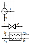 | |||
| Throttle valve 2 | ||||
| Cascade condenser | ||||
| Ethylene Cycle | LP compressor |  | ||
| HP compressor | ||||
| Cooler |  | |||
| Throttle valve 1 | ||||
| Economizer | 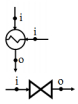 | |||
| Throttle valve 2 | ||||
| Evaporator |  | |||
| Cascade Cycle | ||||
Exergy losses are generated in all system components. Thus, the total exergy losses,
| $\begin{gathered} \Delta \dot E{x_{{\text{tot}}}} = \Delta \dot E{x_{{\text{RC1}}}} + \Delta \dot E{x_{{\text{RC2}}}} + \Delta \dot E{x_{{\text{RCOND}}}} + \Delta \dot E{x_{{\text{RV1}}}} + \Delta \dot E{x_{{\text{RECON}}}} + \hfill \\ \begin{array}{*{20}{c}} {}&{}&{} \end{array}\Delta \dot E{x_{{\text{RV2}}}} + \Delta \dot E{x_{{\text{CC}}}} + \,\Delta \dot E{x_{{\text{EC1}}}} + \Delta \dot E{x_{{\text{EC2}}}} + \Delta \dot E{x_{{\text{EC}}}} + \hfill \\ \begin{array}{*{20}{c}} {}&{}&{} \end{array}\Delta \dot E{x_{{\text{EV1}}}} + \Delta \dot E{x_{{\text{EECON}}}} + \Delta \dot E{x_{{\text{EV2}}}} + \Delta \dot E{x_{{\text{EEVAP}}}} \hfill \\ \end{gathered} $ | (21) |
In the absence of experimental data, or a relevant suitable model for ethylene BOG re-liquefaction systems, the accuracy of the present thermodynamic model was assessed by comparing the performance of a simple cascade refrigeration cycle with that obtained using the free software CoolPack (Skovrup et al., 2012). Calculations were conducted with assumption of the following conditions:
● For the low stage (ethylene) cycle, the evaporation temperature is fixed at-100°C and the condensation temperature at-30°C;
● For the high stage (refrigerant) cycle, the evaporation temperature is fixed at-40°C and the condensation temperature at 40°C;
● The ethylene capacity is fixed at 100 kW;
● Zero superheat and subcooling are used for both cycles. The compression processes are assumed as isentropic, neglecting heat and pressure losses.
It was found that regardless of the nature of refrigerant used in the high pressure branch, the discrepancy between the performance obtained using the CoolPack software and that obtained using the set of state equations developed in the present study did not exceed 3.5%. The only exception was the difference between the two codes when predicting the ethylene mass flow rate (6.73 %), as shown in Table 3. This is a somewhat high relative error, but it is still within the acceptable range for industrial applications and can be attributed to the reduced amount of data used in developing t-he ethylene equations of state at very low temperatures. However, the currently developed program presents the advantage of being more flexible in determining the system performance for different operating conditions.
| R290/R1150 | CoolPack | 0.3434 | 0.7384 | 63.23 | 88.32 | 1.582 | 1.848 |
| Present Model | 0.3203 | 0.7483 | 65.35 | 88.79 | 1.530 | 1.860 | |
| Relative error/% | 6.73 | 1.34 | 3.35 | 0.53 | 3.29 | 0.65 | |
| R600a/R1150 | CoolPack | 0.3434 | 0.8233 | 63.23 | 87.78 | 1.582 | 1.860 |
| Present Model | 0.3203 | 0.8025 | 65.35 | 85.87 | 1.530 | 1.925 | |
| Relative error/% | 6.73 | 2.53 | 3.35 | 2.17 | 3.29 | 3.49 | |
| R1270/R1150 | CoolPack | 0.3434 | 0.7018 | 63.23 | 86.72 | 1.582 | 1.882 |
| Present Model | 0.3203 | 0.7095 | 65.35 | 87.71 | 1.530 | 1.885 | |
| Relative error/% | 6.73 | 1.10 | 3.35 | 1.14 | 3.29 | 0.16 |
Following the above validation study, the developed FORTRAN program was then used to calculate the system performance, thereby enabling comparisons between different working fluids and several operating conditions. The performance of the system, including the power consumed by compressors, the coefficient of performance, the individual exergy losses, the total exergy losses, and the exergy efficiency, were determined by varying the operating parameters and the working fluid of the refrigerant cycle. The main parameters used in analysis are listed in Table 4. The performances of the cascade system were assessed by varying the tank temperature, refrigerant condensation temperature, and the temperature difference in the cascade condenser.
| Parameter | Ethylene | Refrigerant |
| Evaporating temperature/℃ | -103 | -40 |
| Condensation temperature/℃ | -30 | 40 |
| Superheat/℃ | 65 | 10 |
| Subcooling/℃ | 35 | 5 |
| Isentropic compressors efficiency/% | 80 | 80 |
| T3/℃ | 50 | 30 |
| T5/℃ | 30 | - |
Fig. 2(a) illustrates the influence of the tank temperature on the amount of power consumed by the compressors for the refrigerants R290, R600, R600a, and R1270. The tank temperature was varied from 170 to 176 K, while all others parameters were kept constant. For all refrigerants, the increase in tank temperature resulted in an increase in the power consumed by the compressors. This increase can be attributed to a rise of the mass flow rate for both ethylene and refrigerants. As can be observed from the figure, the compressors using R600 and R600a consume less power in comparison to those using R290 and R1270 as operating fluids. It is interesting to note that the use of R1270 would result in a much greater power consumption, while consumption using R290 would be at an intermediate level.

|
| Figure 2 Effect of tank temperature |
Fig. 2(b) depicts the effect of tank temperature on the system’s Coefficient Of Performance (COP). As can be observed from the figure, the increase in tank temperature results in a linear increase in the COP. In fact, a higher tank temperature increases both the power consumed by the compressors and the ethylene evaporation rate. However, the percentage increase in the ethylene evaporation rate is higher than the increase in the power consumed by compressors, which leads to an improvement in the COP. As is clearly visible from the figure, R600 and R600a exhibit practically the same COP as a function of the tank temperature. Therefore, systems operating with these refrigerants are the best in relation to the COP, while systems operating with R1270 produce the lowest COP of all the fluids.
The performance relating to the refrigerants used was then compared using the exergy analysis concept, and the results are presented in Fig. 3(a) and (b) in terms of total exergy losses and exergy efficiency, respectively. For all refrigerants used, the first observation made is that within the range of the operating parameters considered. However, the total exergy loss and the exergy efficiency exhibit a somewhat special behavior: there is an increase in both when the tank temperature is increased. This behavior has been previously reported in others applications using exergy analysis (see for example; Ouadha et al., 2008; Djermouni and Ouadha, 2014). The rise in tank temperature increases both total exergy loss and exergy efficiency, and this was found for all the refrigerants used. Hence, it can be concluded that from an exergy point of view, R600 and R600a again deliver a superior performance compared to R290 and R1270.

|
| Figure 3 Effect of tank temperature |
The variation in refrigerant condensation temperature was also used to analyze the system’s performance, and results were obtained for condensation temperatures ranging from 25 to 40°C, while the other parameters were kept constant. It was found that the power consumed by the compressors of the system increased with a rise in refrigerant condensation temperature. This increase was mainly due to the larger enthalpy difference between the inlet and outlet within the compressors of the refrigerant cycle. Systems using R600 and R600a consumed comparable amounts of energy, but still with lower values compared to other refrigerants. However, in agreement with the above mentioned findings, the energy consumed by a system using R290 is at an intermediate level, whereas that using R1270 as refrigerant uses the largest amount of power, as shown in Fig. 4(a).

|
| Figure 4 Effect of refrigerant condensation temperature |
The combined effect of both the condensation temperature and the nature of the working fluid used in the refrigeration cycle on the coefficient of performance of the system is shown in Fig. 4(b). In general, the COP of the system declines with an increase in the condensation temperature of the refrigeration cycle. However, of all the refrigerants studied, R600a provides by far the highest COP, and this is followed in order by R600, R290, and R1270.
Figs. 5(a) and (b) show the effect of the condensation temperature on the total exergy loss and the exergy efficiency, respectively. Regardless of the refrigerant used, the increase in refrigerant condensation temperature was observed to cause deterioration in the system’s performance: the total exergy loss increased while the exergy efficiency decreased. It is worth mentioning here that the results of both are consistent, as a decrease in the total system exergy loss entails an enhancement in the system exergy efficiency. However, when exergy efficiency is considered, R600a refrigerant remains the best choice.

|
| Figure 5 Effect of refrigerant condensation temperature |
Figure 6 illustrates the percentage of total system exergy destroyed in each component for each refrigerant. For all of the refrigerants, the cascade condenser showed the highest exergy loss contribution (22%–24%), followed in order by the ethylene cooler (11%–12%), refrigerant condenser (10%–11%), high-pressure refrigerant compressor (6.8%–9.9%), refrigerant economizer (6.3%–9.2%), ethylene economizer (6.6%–7.5%), refrigerant valve 2 (6.1%–7.1%), ethylene high-pressure compressor (5%–5.7%), refrigerant low-pressure compressor (4.3%–4.9%), ethylene low-pressure compressor (3.5%–4%), ethylene valve 2 (3%–3.4%), ethylene evaporator (0.82%–4%), refrigerant valve 1 (2%–3.4%), and ethylene valve 1 (1.3%–1.4%). Overall, the exergy losses in the system were mainly due to heat transfer through a finite temperature difference, the irreversible nature of compression, throttling processes, and friction.

|
| Figure 6 Distribution of exergy loss within system: a.R290; b. R600; c. R600a; d. R1270 |
Finally, using the data presented in Table 4, the system performances were evaluated for three temperature differences in the cascade condenser, where the temperature differences considered were 5, 10, and 15°C. The temperature difference in the cascade condenser is defined as the difference between the ethylene condensation temperature and the refrigerant evaporation temperature. Table 5 shows how this temperature difference in the cascade condenser affected the system performance. The resulting data suggest that an increase in the temperature difference within the cascade condenser negatively affects the system’s performance, regardless of the refrigerant used, but that when this temperature difference is smaller the exergy efficiency is improved and less exergy loss occurs in the system. In addition, the power supplied to the system for driving the compressors incrases, together with the total exergy loss, while the COP deteriorates.
| Refrigerant | COP | ||||
| R290 | 5 | 229.62 | 0.61 | 146.66 | 36.23 |
| 10 | 233.09 | 0.59 | 148.72 | 36.20 | |
| 15 | 236.15 | 0.57 | 150.73 | 36.17 | |
| R600 | 5 | 219.81 | 0.64 | 136.51 | 37.90 |
| 10 | 223.69 | 0.62 | 138.99 | 37.87 | |
| 15 | 227.17 | 0.59 | 141.44 | 37.74 | |
| R600a | 5 | 217.97 | 0.65 | 135.00 | 38.07 |
| 10 | 221.93 | 0.62 | 137.54 | 38.02 | |
| 15 | 225.49 | 0.60 | 140.06 | 37.89 | |
| R1270 | 5 | 239.45 | 0.59 | 155.91 | 35.06 |
| 10 | 242.51 | 0.57 | 157.59 | 35.02 | |
| 15 | 245.14 | 0.55 | 259.19 | 34.89 |
A thermodynamic analysis is conducted to compare the performance of hydrocarbon refrigerants in an ethylene re-liquefaction system, where the refrigerants considered are R290, R600, R600a, and R1270. Overall, results show that the performances of the ethylene re-liquefaction system are proportional to the operating parameters and the working fluid in the refrigeration subsystem. The main conclusions obtained from the present study are summarized as follows.
1) R600a gives the best refrigerant performance, and is followed in order by R600, R290, and R1270.
2) There are very small differences between the use of R600 and R600a, both in terms of COP and exergy efficiency.
3) An increase in tank temperature increases the performance of the system.
4) An increase in condensation temperature causes deterioration of the system’s performance.
5) Individual exergy losses can be categorized into three groups according to percentage contribution to total exergy loss: an upper group (
6) Within the considered variation range of tank temperature, the total exergy loss and the exergy efficiency of the system exhibit a special behavior: both increase with a rise in tank temperature.
7) The system performs better if the temperature difference in the cascade condenser is kept low.
| Anderson TN, Ehrhardt ME, Foglesong RE, Bolton T, Jones D, Richardson A, 2009.Shipboard reliquefaction for large LNG carriers.Proc. 1st Annual Gas Processing Symposium, Doha, Qatar. |
| Baek S, Hwang G, Lee C, Jeong S, Choi D, 2011. Novel design of LNG (liquefied natural gas) reliquefaction process. Energy Conversion Management, 52(8-9), 2807–2814. DOI:10.1016/j.enconman.2011.02.015 |
| Beladjine MB, Ouadha A, Adjlout L, 2013. Performance analysis of oxygen refrigerant in an LNG BOG re-liquefaction plant. Procedia Computer Science, 19, 762–769. DOI:10.1016/j.procs.2013.06.100 |
| Beladjine BM, Ouadha A, Benabdesslam Y, Adjlout L, 2011. Exergy analysis of an LNG BOG re-liquefaction plant.Proc. 23rd IIR Int. Congress Refrigeration, Prague, Czech Republic. |
| Berlinck EC, Parise JAR, Pitanga Marques R, 1997. Numerical simulation of an ethylene re-liquefaction plant. Int. J. Energy Research, 21(7), 597–614. DOI:10.1002/(SICI)1099-114X(19970610)21:7 < 597::AID-ER193 > 3.0.CO; 2-5 |
| Bosnjakovic F, 1965. Technical thermodynamics. New York: Holt, Rinehartand Winston. |
| Bounefour O, Ouadha A, 2014.Thermodynamic analysis and working fluid optimization of a combined ORC-VCC system using waste heat from a marine diesel engine.Proc. ASME 2014 Int. Mechanical Eng. Congress Exposition, Montreal, Canada. |
| Brodyansky VM, Sorin MV, Le Goff P, 1994. The efficiency of industrial processes:exergy analysis and optimization. New York: Elsevier. |
| Chien MH, Shih MY, 2011. An Innovative optimization design for a boil-off gas reliquefaction process of LEG vessels. J. Petroleum, 47(4), 65–74. |
| Chin YW, 2006. Cycle analysis on LNG boil-off gas re-liquefaction plant. J.Korean Institute Appl. Superconductivity Cryogenics, 8(4), 34–38. |
| Dimopoulos GG, Frangopoulos CA, 2008. A Dynamic model for liquefied natural gas evaporation during marine transportation. Int. J. Thermodynamics, 11(3), 123–131. DOI:10.5541/ijot.220 |
| Djermouni M, Ouadha A, 2014. Thermodynamic analysis of an HCCI engine based system running on natural gas. Energy Conversion Management, 88(12), 723–731. DOI:10.1016/j.enconman.2014.09.033 |
| Gomez JR, Gomez MR, Bernal JL, Insua AB, 2015. Analysis and efficiency enhancement of a boil-off gas reliquefaction system with cascade cycle on board LNG carriers. Energy Conversion Management, 94(4), 261–274. DOI:10.1016/j.enconman.2015.01.074 |
| Kotas TJ, 1985. The exergy method of thermal plant analysis. London: Butterworth. |
| Li Y, Jin G, Zhong Z, 2012. Thermodynamic Analysis-based improvement for the boil-off gas reliquefaction. Process of Liquefied Ethylene Vessels, Chemical Eng. Technology, 35(10), 1759–1764. |
| Moon JW, Lee YP, Jin YW, Hong ES, Chang HM, 2007. Cryogenic refrigeration cycle for re-liquefaction of LNG boil-off gas. Int. Cryocooler Conference, Boulder, 629-635. |
| Moran MJ, Shapiro HN, 2000. Fundamentals of engineering thermodynamics. New York: Wiley. |
| Nanowski D, 2012. Gas plant of ethylene gas carrier and a two stages compression optimization of ethylene as a cargo based on thermodynamic analysis. J. Polish CIMAC, 7(1), 183–190. |
| Ouadha A, En-nacer M, Adjlout L, Imine O, 2005. Exergy analysis of two-stage refrigeration cycle using two natural substitutes of HCFC 22. Int. J. Exergy, 2(1), 14–30. DOI:10.1504/IJEX.2005.006430 |
| Ouadha A, En-nacer M, Imine O, 2008. Thermodynamic modelling of a water-to-water heat pump using propane as refrigerant. Int. J. Exergy, 5(4), 451–469. DOI:10.1504/IJEX.2008.019115 |
| Ouadha A, Haddad C, En-nacer M, Imine O, 2007. performance comparison of cascade and two-stage refrigeration cycles using natural refrigerants. Beijing, China: Int. Congress Refrigeration. |
| Pil CK, Rausand M, Vatn J, 2008. Reliability assessment of reliquefaction systems on LNG carriers. Reliability Eng. System Safety, 93(9), 1345–1353. DOI:10.1016/j.ress.2006.11.005 |
| Romero J, Orosa JA, Oliveira AC, 2012. Research on the Brayton cycle design conditions for reliquefaction cooling of LNG boil off. J. Marine Science Technology, 17(4), 532–541. DOI:10.1007/s00773-012-0180-3 |
| Sayyaadi H, Babaelahi M, 2010. Thermoeconomic optimization of a cryogenic refrigeration cycle for re-liquefaction of the LNG boil-off gas. Int. J. Refrig., 33(6), 1197–1207. DOI:10.1016/j.ijrefrig.2010.03.008 |
| Shin Y, Lee YP, 2009. Design of a boil-off natural gas reliquefaction control system for LNG carriers. Appl. Energy, 86(1), 37–44. DOI:10.1016/j.apenergy.2008.03.019 |
| Skovrup MJ, Jakobsen A, Rasmussen BD, Andersen SE, 2012. CoolPack (Version: 1.5). Available from: http://en.ipu.dk/Indhold/refrigeration-and-energy-technology/coolpack.aspx |
| Syechev VV, 1983. Les equations différentielles de la thermodynamique. Edition Mir, Moscou. |