 2018, Vol. 38


随着我国城镇化进程的加快, 部分地区不合理的土地利用和污染物排放, 引起了很多不合理的水资源开发, 带来了城市及周边河流与湖泊的富营养化、城市水体水质恶化、湿地生态功能退化等一系列城市水生环境问题(丁惠君等, 2017), 这不仅影响了人们的日常生活, 同时制约了沿海地区流域经济的可持续发展.城市湖泊的水质优劣, 在很大程度上可以影响一个城市是否“山清水秀”的意识与具体形象(丁惠君等, 2017; 郑田甜等, 2018).总悬浮物(Total Suspended Matter, TSM)是水体的光学敏感组分和评价水质的重要指标之一, 对湖泊水环境评价、水体物质迁移转化、沉积物埋藏动力具有重要的意义(Cole and Cloern, 1987).水中TSM浓度能够很大程度上决定水体的透明度、浑浊度、水色等光学性质(Cole and Cloern, 1987; May et al., 2003), 既直接影响湖泊水体的视觉观感, 也会影响其初级生产力及水生植被的生长(Zhang et al., 2014).因此, 为了理解、管理和保护湖泊生态系统, 迫切需要获取长期TSM的时空信息.
过去由欧美科学家主导的湖沼学多是面向淡水生物学或生态学, 主要研究对象是各类湖泊, 主要方法是实地采样和分析(Kalff, 2002).这种方法耗费的人力物力较大, 并且主要是对特定时段的特定区域进行观测.通过这种方法获取的TSM值相对精确, 但由于采样点的局限性, 测量结果往往难以准确反映研究区域的整体水质状况, 并且难以实现TSM的实时动态监测(Wang et al., 2007).为了解决传统方法的局限性, 可以通过光学遥感技术克服传统方法所面临的问题, 在大范围反演水体的TSM状况.自1972年首次发射Landsat卫星以来, 这类方法已被广泛用于获取TSM的时空信息(Miller and Mckee, 2004).
目前, 有很多研究利用高时间分辨率的海洋水色卫星分析大湖TSM浓度的时空变化, 例如太湖(Zhang et al., 2014)、东海(Mao et al., 2012)、鄱阳湖(Cui et al., 2013)和洞庭湖(Wu et al., 2014).也有利用Landsat系列卫星研究大湖TSM浓度的小尺度变化, 例如太湖(Zhou et al., 2006; Ma and Dai, 2005).与大型湖泊相比, 城市中小型湖泊水体的生物-光学特征相对复杂, 空间尺度较小, 易受人类活动影响(Aurin et al., 2013).海洋水色卫星的低空间分辨率(300~1000 m)显然不能有效地探测城市湖泊小尺度的水质变化(Palmer et al., 2015), 而国内外基于以往Landsat系列卫星的TSM浓度研究则主要集中在高悬浮物浓度水体, 例如太湖(马荣华等, 2005)、Frisian湖区(Dekker et al., 2001).学者通过比较不同悬浮物浓度的光谱曲线发现, 690~900 nm波段的水体反射随悬浮物浓度的增加而增加, 因此比较适合用于反演悬浮物浓度.但对于较清洁的水体, 反射率在该波段范围内的变化并不明显, 因而限制其方法的进一步应用(张毅博等, 2015).Landsat-8于2013年2月发射, 以相对较高的空间分辨率(30 m)继续Landsat的地球观测任务(Pahlevan et al., 2014). Landsat-8在数据质量和频谱覆盖方面都有着显着的改进(12位的量化等级和提高的信噪比以及增设的海岸带/气溶胶(Coastal Aerosol)波段) (Chen et al., 2017).近期一些研究已经开始利用Landsat-8获取沿海及内陆水域的水质参数(Li et al., 2015; Chen et al., 2017; Zhang et al., 2016; Kim et al., 2014), 展现了Landsat面向小尺度水体TSM浓度的研究潜力(Cai et al., 2015; Urbanski et al., 2016; Lymburner et al., 2016), 但其反演方式大都是运用经验统计模型, 具有一定的局限性, 具体的模型方式和参数不适用于特定城市湖泊水体.
文献调研发现以往对于悬浮物的遥感研究大部分是关于悬浮物浓度估算, 而悬浮物吸收系数的研究较少.但水色遥感中, 与遥感反射率直接关联的是物质的光学属性, 即其吸收和反射特性(表现为吸收系数和后向散射系数), 而且根据Beer′s Low, 水中物质的浓度往往和其光学特征有较强的相关性, 因此利用悬浮颗粒的吸收系数来指示其浓度是有依据的.常规的TSM遥感研究是通过光谱直接反演浓度, 这类方法实际上就假设了悬浮颗粒的光学属性和其物质浓度之间存在良好的相关性.事实上, 在水色遥感中, 很多算法都是反演出水体组分的吸收系数, 例如黄色物质(aCDOM)和叶绿素(aph)(Le et al., 2011; Chen et al., 2017), 如果需要确切知道这些物质的浓度大小, 只需要建立其浓度(g·L-1)和吸收系数之间的相关函数即可.因此, 在水质遥感中, 用TSM吸收系数来代表TSM浓度也是准确可行的, 通过对ap(440)的研究反映TSM浓度的变化情况(Astoreca et al., 2012; Kirk, 1994).利用遥感估算TSM浓度的方法主要有分析法(Zhang et al., 2008)、半分析法(施坤等, 2011)和经验法(Xi and Zhang, 2011; 张毅博等, 2015), 前人研究表明经验法简单, 易于构建, 而且在一定程度上可以降低大气校正误差带来的影响(Xi and Zhang, 2011).许多研究使用了经验模型(马荣华等, 2005; Dekker et al., 2002)来估计TSM浓度, 模型输入包括单波段、波段组合.
杭州西湖以其良好的生态环境、独特的风景和悠久的人文历史闻名于世.但随着人口压力的增加、旅游人数的增多(估计每年有4000万人访问西湖(Torbick et al., 2008))、社会经济发展及资源的开发利用, 西湖水体水质长期面临着富营养化等问题(尤爱菊等, 2015).数十年来杭州市投入了大量的人力、物力和财力开展西湖的综合整治工作, 包括湖底疏浚、入湖溪流整治、西湖西进、引配水、水域生态修复等措施.西湖实施综合整治及大规模引水配水后, 入湖污染负荷得到了有效控制, 水体更新能力增强, 水环境改善趋势明显(尤爱菊等, 2015).近年来, 有关西湖水质、富营养化和生态因子的监测评价成果较多(Cai et al., 2012; 李琳琳等, 2013), 而利用遥感方法针对西湖时间分段和空间分区的水质变化特征、驱动因素研究成果较少.目前杭州西湖的叶绿素的变化已有报道(Torbick et al., 2008), 但用Landsat-8遥感研究西湖的TSM还未见报道.
本研究的目的是运用遥感反演的手段评估西湖的水质参数TSM吸收系数的状况.结合水质采样数据和Landsat-8遥感影像数据, 根据实地采样数据进行高光谱建模.通过比较不同经验函数形式和不同模型输入的效果, 得到高光谱下的最佳函数模型.由模型建模的R2示意图, 分析西湖TSM吸收系数的光学吸收特征, 估算其光学敏感波段范围, 可以看到最佳函数的最佳波段组合范围.在高光谱建模基础上, 对比高光谱最佳函数的模型输入波段范围和Landsat-8的波段设置, 利用两者相匹配的单波段或波段组合来开发模型.之后进行同步卫星数据验证, 并在图像上应用模型, 观察TSM吸收系数在西湖不同空间和时间季节的分布变化, 初步探索自然环境因素和人为活动对西湖水质的影响, 为后续的城市湖泊水质研究和杭州西湖的综合管理提供科学依据.
2 数据和方法(Data and methods) 2.1 研究区域西湖(120°08′E, 30°15′N)位于中国东南沿海的杭州市西侧, 是我国典型的游览型湖泊.西湖东面靠近市区, 其他三面环山, 其东西长度约为2.8 km, 南北长度约为3.3 km, 水域面积约为5.66 km2.它是一个浅水湖泊, 平均深度1.75 m, 总体积约16 km3 (Torbick et al., 2008).俯视看, 西湖的水与其他水域似乎是隔绝开来的, 但实际上其西南部有多个入水口, 钱塘江是南端入湖淡水的主要来源, 在其北面拥有数个出水口, 这样使得西湖并非全封闭湖泊, 水体的更新度较好.西湖各水域之间是半封闭的, 主要通过桥洞进行水的置换.因此其各自的水质一定程度上独立.西湖北面和东面靠近市区, 人为活动频繁.西面和南面是自然风景区, 人为活动较北面和东面少.在2017年, 杭州市国内旅游人数从春(3058万人)开始逐渐增加, 夏季4186万人, 直到秋季(5086.9万人)到达顶峰, 然后在冬季下降(杭州统计信息网).旅游对西湖水质的影响不容忽视.
 |
| 图 1 采样点分布示意图 Fig. 1 The distribution of sampling points |
2017年7月20—27日和2017年9月18日在杭州西湖地区进行了两次野外采样, 分别收集了28个样本和22个样本(共50个).使用美国ASD公司生产的ASD FieldSpec HandHeld2手持式地物光谱仪(325~1075 nm, 波长采样间隔1 nm)在晴天无云和少云情况下收集实地水表面的光学特性(NASA的规范).使用采水器收集水表面样品, 将其装配到琥珀瓶(聚丙烯250 mL)中, 并储存在冷却器中, 直到在实验室中进一步分析.对于每个采样点, 测量10个光谱以最小化不确定性, 并计算Rrs(式(1)).
|
(1) |
式中, ρ是水表面反射系数, Lg是白板辐亮度, Lsky是天空光辐亮度, Rt是水面总反射率.根据ASD指导手册和Mobley(1999)推荐值, 本研究中ρ设置为0.028.
在实验室中, 水样在低压下(< 5 atm)通过玻璃微纤维膜(0.45 μm)进行过滤, 收集滤液.然后使用美国Agilent公司生产的Cary 100 UV-Vis分光光度计测定摇晃过的原液和滤液在200~800 nm范围的吸光度A(λ).然后, 将两者的吸光度分别转换成吸收系数(式(2)和式(3)).
|
(2) |

|
(3) |
式中, Pathlength是比色皿的宽度, 为1 cm.将aTotal与aCDOM相减(式(4)), 即得TSM的吸收系数(ap).
|
(4) |
本研究中, 使用Landsat-8 OLI图像.Landsat-8卫星具有两个传感器:OLI(Operational Land Imager)和TIRS(Thermal Infrared Sensor)热红外传感器, 时间分辨率是16 d. OLI是一种推扫式成像扫描仪, 有9个波段, 其中8个波段的空间分辨率是30 m, 全色波段的空间分辨率是15 m(Irons et al., 2012).它提供了5个可用于内陆水域遥感的可见波段:B1(沿海/气溶胶:433~453 nm), B2(蓝色:450~515 nm), B3(绿色:525~600 nm), B4(红色:630~680 nm)和B5(近红外:850~880 nm).
本研究从美国地质调查局(USGS)官网(www.earthexplorer.usgs.gov)下载了4幅Landsat-8 OLI C1 Level2影像(行列号:119, 39), 其中2017年9月16日的影像用于数据验证, 另外3幅用于观测TSM时空变化.Landsat-8影像2级产品采用的是6S(Second Simulation of Satellite Signal in the Solar Spectrum)辐射传输模型进行大气校正, 进一步处理得到Rrs产品.
2.3 算法开发和精度评估 2.3.1 高光谱算法开发与评估本研究中, 实地测量的光谱被用来建立经验模型.通过使用线性, 指数和对数函数来测试所有可能的单波段和波段组合形式.从而建立最佳经验模型.
|
(5) |
式中, x是波段的各种组合(取400~900 nm波段), y是ap(440).根据建模流程, 共有2260512个波段组合(单波段:3个函数×501波段输入, 双波段:3种函数×3种波段组合×251001波段输入), 但其中存在一些无效组合(9个函数×501)和重复组合(6个函数×125250个).最终只构建了1504503个波段组合(表 1).
| 表 1 模型结果统计分析 Table 1 Statistical analysis of model results |
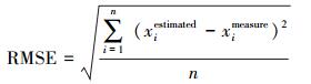
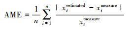
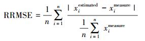
通过模型精度评估, 获取最佳波段输入模型.首先从50个样本中随机抽取35个样本(建模数据组)构建模型, 使用剩下的15个样本对其进行验证.根据建模/验证数据组的R2、RMSE、AME和RRMSE对各个模型进行比较.它们的公式定义如下:
|
(6) |
|
(7) |
|
(8) |
对于TSM, 我们只记录了给出RMSE、AME和RRMSE最小的或R2最大的两个最佳函数模型.因此, 对于总共1504503个模型, 最终获得了2个最佳函数模型供进一步分析.确定高光谱情况下的最佳函数模型.再画出模型的波段组合建模的R2示意图, 可以看到最佳函数的最佳波段组合范围.
2.3.2 Landsat-8算法开发与评估利用2017年9月16日的Landsat-8卫星图像进行验证.影像时间比实测早2 d.从Landsat 4/5/7/8(Tebbs et al., 2013; Mccullough et al., 2012; Lobo et al., 2015)的算法校准和验证结果来看2 d仍然是可接受的时间范围.另外, 在这2 d内, 没有发生对水质变化有影响的天气或人为事件, 如强风、降水、温度变化, 河流或湖岸建设项目, 因此水质没有显著变化.本研究取每个实测位置为中心的3×3像素矩阵窗口的中值来作为采样点的卫星Rrs.此外, 由于当天卫星数据部分区域有云, 22个采样点中只有10个没有被云覆盖的点能用于卫星验证.10个样本在OLI3和OLI4的大气校正误差为22.45%和22.19%.在高光谱建模基础上, 对比高光谱最佳函数的模型输入波段范围和Landsat-8的波段设置, 利用两者相匹配的单波段或波段组合来开发模型.利用Landsat-8的光谱响应函数对实地光谱进行处理, 然后利用生成的波段进行建模(Chen et al., 2017).将50样本点同高光谱建模一样, 分为建模集(35样本)和验证集(15样本).评估标准同样采用RMSE、AME、RRMSE和R2.
3 结果与讨论(Results and discussion) 3.1 实测水质和光谱本研究中使用的数据主要是aTotal、aCDOM和ap, 来自两次采样活动.图 2是50个采样点的aCDOM(440), ap(440)数据, 其中aTotal(440)的范围是2.34~20.50 m-1, aCDOM(440)值相对较小, 范围是0.05~1.15 m-1.ap是aTotal与aCDOM的差值, 计算的ap(440)的范围是2.02~19.81 m-1.
 |
| 图 2 采样点的吸收系数aCDOM(440), ap(440) Fig. 2 The aCDOM(440), ap(440) of sampling point |
由于光谱在900 nm附近迅速下降, 接近0, 数据的信噪比降低, 并且具有较大的噪声, 因此本研究只对400~900 nm范围的光谱数据进行分析.实测Rrs有典型的内陆水体光谱特征(图 3):在570 nm处的反射峰主要是由于叶绿素和胡萝卜素在该波段附近的弱吸收及细胞的散射作用形成的(刘忠华等, 2011); 670 nm左右由于叶绿素a的吸收形成一个较小的反射谷(Bidigare et al., 1990); 700 nm左右存在一个明显的叶绿素荧光峰(Gitelson, 1992).
 |
| 图 3 采样点实地光谱 Fig. 3 The field spectrum of sampling point |
如上所述, 通过对模型进行精度评估可以确定最优的模型.表 2表明, 使用Rrs数据构建模型, 最佳输入通常是B1/B2或(B1-B2)/(B1+B2), 最佳函数形式是y=a·eb·x.
| 表 2 模型反演的ap(440)和原位测量的ap(440)的比较 Table 2 Comparison of the model inversion ap(440) and the in situ measured ap(440) |
结合表 1中建模集的R2和验证集RMSE、AME、RRMSE, 输入B1/B2应该被认为是建模的最好波段输入, (B1-B2)/(B1+B2)可作为第二选择.
3.3 确定最佳波段范围如2.2节所述, 最佳模型输入是指数函数形式下的B1/B2或(B1 - B2)/(B1+B2). 图 4a、4b)表明用B1/B2作为指数模型输入, B1选用600~720 nm范围波段, B2选用500~535 nm范围波段, 可使模型R2 > 0.6, RMSE < 4.图 4c、4d)表明用(B1-B2)/(B1+B2)作为指数模型输入, B1选用700~730 nm范围波段, B2选用500~620 nm范围波段, 可使模型R2 > 0.6, RMSE < 4.
 |
| 图 4 y=a·eb·(B1/B2)和y=a·eb·(B1-B2)/(B1+B2)模型各波段R2>0.60和RMSE < 4图 Fig. 4 y=a·eb·(B1/B2) and y=a·eb·(B1-B2)/(B1+B2) model R2> 0.60 chart and RMSE < 4 chart for each band |
通过比较Landsat-8波段范围和最佳波段组合范围(2.3节), 最好的波段组合是红波段与绿波段.前人研究同样表明, 反演TSM一般采用绿光, 红光波段或近红外波段(Doxaran et al., 2002; Binding et al., 2005).
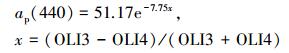
基于上述结果, 我们建议使用基于OLI4 / OLI3(红波段/绿波段)的指数模型作为Landset-8的ap估计的最佳模型, 其在建模和验证中给出了最好的结果(R2 = 0.82, RMSE = 2.05 m-1, 图 5a、5b所示).公式为

|
(9) |
 |
| 图 5 OLI4 / OLI3和(OLI3-OLI4)/(OLI3+OLI4)模型拟合图和验证集对比图 Fig. 5 OLI4 / OLI3 and(OLI3-OLI4)/(OLI3+OLI4) model fitting chart and verification comparison chart |
一个替代模型是以(OLI3-OLI4)/(OLI3+OLI4)为基础的模型, 此模型也具备了良好的预测性能(R2= 0.81, RMSE = 2.12 m-1, 图 5c、5d).公式如下:
|
(10) |
从RMSE来看, (OLI3-OLI4)/(OLI4+OLI3)模型(RMSE= 6.17 m-1, AME=66%)略好于OLI4 / OLI3模型(RMSE = 8.18 m-1, AME=72%), 误差较小(表 2).样本5的误差较大, 该点比较靠近岸边, 因此, 2017年9月18日的现场采样可能和卫星过境拍摄图像的水质有一定的差异性.公式(9)被应用于图像, 得到如图 6所示的TSM空间分布.
 |
| 图 6 西湖2017年1月3日(a)、7月14日(b)、9月16日(c)和11月3日(d) ap(440)吸收系数反演结果 Fig. 6 The maps of ap(440) absorption coefficient on Jan 3, Jul 14, Sep 16 and Nov 3, 2017 of Lake West |
2017年1月3日、7月14日和11月3日的3幅影像被用于估算ap(440)(图 6).根据图像得出的结果(表 3), 7月份TSM吸收系数偏高可能是由于两方面的原因:一方面是水生生物生长, 导致藻类悬浮物增多;一方面是由于西湖夏季旅游人数增多, 游船来往次数增加, 导致湖水频繁搅动, 引起底泥等物质上浮, 造成非藻类悬浮物增多.藻类和非藻类悬浮物同时增多, 从而引起TSM吸收系数增高.而9月吸收系数降低的原因在一定程度上可能是由于旅游人数回落以及秋季降雨量的增多.除此之外, 还可能是由于7月和8月阳光充足, 水生植物生长消耗营养盐过多, 导致9月其生长进入停滞阶段, 造成藻类颗粒减少.主湖区域中较高的TSM吸收系数与现场测量结果一致.在视觉上, 主湖和北里湖区域的人类活动较多, 所以悬浮物吸收系数较高.并且由于其南进水口, 北出水口的位置, 使得悬浮物从北到南, 吸收系数逐渐降低.
| 表 3 西湖各区域TSM吸收系数ap(440)统计比较 Table 3 Statistics and comparison of ap(440) in various regions of the West Lake |
反演得到的图像表明使用悬浮物监测水质具有潜在价值.例如2017年7月14日西里湖有一块高TSM区域.这块区域很可能是由于岸边的人为活动所导致.这块区域相对较小, 在一般的卫星影像中很难被观测到.
4 结论(Conclusions)1) 通过对高光谱变量与TSM吸收系数进行建模分析, 发现红波段和绿波段为杭州西湖TSM吸收系数估算的敏感波段.
2) 针对杭州西湖提出一个较好的基于Landsat-8的TSM吸收系数估算模型, 该模型具有较好效果, 估算模型为:
|
3) 西湖区域ap(440)整体较低, 平均为15.91~24.7 m-1, 最低为6.99 m-1, 最高为36.53 m-1, 这些高吸收系数部分一般位于湖的边缘区, 主要受入水口、出水口以及湖周围和湖上人类活动的影响区域, 如湖北面出水口附近的ap(440)长期较高, 1月份西湖北边岸边受人类活动影响较大, ap(440)较高.从区域上看, 主湖和北里湖吸收系数较高, 西里湖次之, 整体上从南到北吸收系数逐渐升高, 这可能是受人类活动和入出水口的共同影响.这些分析均是对TSM吸收系数变化原因的初步探索, 更为细致和论据充足的分析, 还需要进一步的研究.
Astoreca R, Doxaran D, Ruddick K, et al. 2012. Influence of suspended particle concentration, composition and size on the variability of inherent optical properties of the Southern North Sea[J]. Continental Shelf Research, 35: 117–128.
|
Aurin D, Mannino A, Franz B. 2013. Spatially resolving ocean color and sediment dispersion in river plumes, coastal systems, and continental shelf waters[J]. Remote Sensing of Environment, 137: 212–225.
DOI:10.1016/j.rse.2013.06.018
|
Bidigare R R, Ondrusek M E, Morrow J H, et al. 1990. In-vivo absorption properties of algal pigments[Z]. International Society for Optics and Photonics. 290-303
|
Binding C E, Bowers D G, Mitchelson-Jacob E G. 2005. Estimating suspended sediment concentrations from ocean colour measurements in moderately turbid waters; the impact of variable particle scattering properties[J]. Remote Sensing of Environment, 94(3): 373–383.
DOI:10.1016/j.rse.2004.11.002
|
Cai L, Tang D, Li C. 2015. An investigation of spatial variation of suspended sediment concentration induced by a bay bridge based on Landsat TM and OLI data[J]. Advances in Space Research, 56(2): 293–303.
DOI:10.1016/j.asr.2015.04.015
|
Cai L, Zhou Q, He F, et al. 2012. Investigation of microbial community structure with culture-dependent and independent PCR-DGGE methods in western west lake of Hangzhou, China[J]. Fresenius Environmental Bulletin, 21(6): 1357–1364.
|
Chen J, Zhu W, Tian Y Q, et al. 2017. Estimation of colored dissolved organic matter from landsat-8 imagery for complex inland water:Case study of Lake Huron[J]. IEEE Transactions on Geoscience and Remote Sensing, 55(4): 2201–2212.
|
Chen J, Zhu W, Tian Y Q, et al. 2017. Remote estimation of colored dissolved organic matter and chlorophyll-a in Lake Huron using Sentinel-2 measurements[J]. Journal of Applied Remote Sensing, 11(3): 36007.
|
Cole B E, Cloern J E. 1987. An empirical model for estimating phytoplankton productivity in estuaries[J]. Marine Ecology Progress Series, 36(1): 299–305.
|
Cui L, Qiu Y, Fei T, et al. 2013. Using remotely sensed suspended sediment concentration variation to improve management of Poyang Lake, China[J]. Lake and Reservoir Management, 29(1): 47–60.
DOI:10.1080/10402381.2013.768733
|
Ding H, Zhong J, Wu Y, et al. 2017. Characteristics and ecological risk assessment of antibiotics in five city lakes in Nanchang City, Lake Poyang Catchment[J]. Journal of Lake Sciences, 29(4): 848–858.
DOI:10.18307/2017.0408
|
Dekker A G, Vos R J, Peters S. 2001. Comparison of remote sensing data, model results and in situ data for total suspended matter (TSM) in the southern Frisian lakes[J]. Science of the Total Environment, 268(1): 197–214.
|
Dekker A G, Vos R J, Peters S. 2002. Analytical algorithms for lake water TSM estimation for retrospective analyses of TM and SPOT sensor data[J]. International Journal of Remote Sensing, 23(1): 15–35.
DOI:10.1080/01431160010006917
|
丁惠君, 钟家有, 吴亦潇, 等. 2017. 鄱阳湖流域南昌市城市湖泊水体抗生素污染特征及生态风险分析[J]. 湖泊科学, 2017, 29(4): 848–858.
|
Doxaran D, Froidefond J, Lavender S, et al. 2002. Spectral signature of highly turbid waters:Application with SPOT data to quantify suspended particulate matter concentrations[J]. Remote Sensing of Environment, 81(1): 149–161.
|
Gitelson A. 1992. The peak near 700 nm on radiance spectra of algae and water:relationships of its magnitude and position with chlorophyll concentration[J]. International Journal of Remote Sensing, 13(17): 3367–3373.
DOI:10.1080/01431169208904125
|
Liu Z, Li Y, Lue H, et al. 2011. Inversion of suspended matter concentration in Lake Chaohu based on partial least-squares regression[J]. Journal of Lake Sciences, 23(3): 357–365.
|
Irons J R, Dwyer J L, Barsi J A. 2012. The next Landsat satellite:The Landsat data continuity mission[J]. Remote Sensing of Environment, 122: 11–21.
DOI:10.1016/j.rse.2011.08.026
|
Kalff J. 2002. Limnology: inland water ecosystems[M], No. 504.45 KAL.
|
Kim S, Kim H, Hyun C. 2014. High resolution ocean color products estimation in Fjord of Svalbard, arctic sea using Landsat-8 oli[J]. Korean Journal of Remote Sensing, 30(6): 809–816.
DOI:10.7780/kjrs.2014.30.6.11
|
Kirk J T. 1994. Light and photosynthesis in aquatic ecosystems[M]. Cambridge: Cambridge University Press.
|
Le C, Li Y, Zha Y, et al. 2011. Remote estimation of chlorophyll a in optically complex waters based on optical classification[J]. Remote Sensing of Environment, 115(2): 725–737.
|
Li J, Chen X, Tian L, et al. 2015. Improved capabilities of the Chinese high-resolution remote sensing satellite GF-1 for monitoring suspended particulate matter (SPM) in inland waters:Radiometric and spatial considerations[J]. ISPRS Journal of Photogrammetry and Remote Sensing, 106: 145–156.
DOI:10.1016/j.isprsjprs.2015.05.009
|
Lobo F L, Costa M P, Novo E M. 2015. Time-series analysis of Landsat-MSS/TM/OLI images over Amazonian waters impacted by gold mining activities[J]. Remote Sensing of Environment, 157: 170–184.
|
Lymburner L, Botha E, Hestir E, et al. 2016. Landsat 8:providing continuity and increased precision for measuring multi-decadal time series of total suspended matter[J]. Remote Sensing of Environment, 185: 108–118.
DOI:10.1016/j.rse.2016.04.011
|
李琳琳, 汤祥明, 高光, 等. 2013. 沉水植物生态修复对西湖细菌多样性及群落结构的影响[J]. 湖泊科学, 2013, 25(2): 188–198.
DOI:10.3969/j.issn.1003-5427.2013.02.003 |
刘忠华, 李云梅, 吕恒, 等. 2011. 基于偏最小二乘法的巢湖悬浮物浓度反演[J]. 湖泊科学, 2011, 23(3): 357–365.
|
Ma R, Dai J. 2005. Investigation of chlorophyll-a and total suspended matter concentrations using Landsat ETM and field spectral measurement in Taihu Lake, China[J]. International Journal of Remote Sensing, 26(13): 2779–2795.
DOI:10.1080/01431160512331326648
|
Mao Z, Chen J, Pan D, et al. 2012. A regional remote sensing algorithm for total suspended matter in the East China Sea[J]. Remote Sensing of Environment, 124: 819–831.
DOI:10.1016/j.rse.2012.06.014
|
May C L, Koseff J R, Lucas L V, et al. 2003. Effects of spatial and temporal variability of turbidity on phytoplankton blooms[J]. Marine Ecology Progress Series, 254: 111–128.
DOI:10.3354/meps254111
|
Mccullough I M, Loftin C S, Sader S A. 2012. Combining lake and watershed characteristics with Landsat TM data for remote estimation of regional lake clarity[J]. Remote Sensing of Environment, 123: 109–115.
|
马荣华, 戴锦芳. 2005. 结合Landsat ETM与实测光谱估测太湖叶绿素及悬浮物含量[J]. 湖泊科学, 2005, 17(2): 97–103.
DOI:10.3321/j.issn:1003-5427.2005.02.001 |
Miller R L, Mckee B A. 2004. Using MODIS Terra 250 m imagery to map concentrations of total suspended matter in coastal waters[J]. Remote sensing of Environment, 93(1): 259–266.
|
Mobley C D. 1999. Estimation of the remote-sensing reflectance from above-surface measurements[J]. Applied Optics, 38(36): 7442–7455.
|
Pahlevan N, Lee Z, Wei J, et al. 2014. On-orbit radiometric characterization of OLI (Landsat-8) for applications in aquatic remote sensing[J]. Remote Sensing of Environment, 154: 272–284.
DOI:10.1016/j.rse.2014.08.001
|
Palmer S C, Kutser T, Hunter P D. 2015. Remote sensing of inland waters: Challenges, progress and future directions[Z]. Elsevier
|
施坤, 李云梅, 刘忠华, 等. 2011. 基于半分析方法的内陆湖泊水体总悬浮物浓度遥感估算研究[J]. 环境科学, 2011, 32(6): 1571–1580.
|
Tebbs E J, Remedios J J, Harper D M. 2013. Remote sensing of chlorophyll-a as a measure of cyanobacterial biomass in Lake Bogoria, a hypertrophic, saline-alkaline, flamingo lake, using Landsat ETM+[J]. Remote Sensing of Environment, 135: 92–106.
DOI:10.1016/j.rse.2013.03.024
|
Torbick N, Hu F, Zhang J, et al. 2008. Mapping chlorophyll-a concentrations in West Lake, China using Landsat 7 ETM+[J]. Journal of Great Lakes Research, 34(3): 559–565.
DOI:10.3394/0380-1330(2008)34[559:MCCIWL]2.0.CO;2
|
Urbanski J A, Wochna A, Bubak I, et al. 2016. Application of Landsat 8 imagery to regional-scale assessment of lake water quality[J]. International Journal of Applied Earth Observation and Geoinformation, 51: 28–36.
DOI:10.1016/j.jag.2016.04.004
|
Wang Y H, Deng Z D, Ma R H. 2007. Suspended solids concentration estimation in Lake Taihu using field spectra and MODIS data[J]. Acta Scientiae Circumstantiae, 27(3): 509–515.
|
Wu G, Liu L, Chen F, et al. 2014. Developing MODIS-based retrieval models of suspended particulate matter concentration in Dongting Lake, China[J]. International Journal of Applied Earth Observation and Geoinformation, 32: 46–53.
|
Xi H, Zhang Y. 2011. Total suspended matter observation in the Pearl River estuary from in situ and MERIS data[J]. Environmental Monitoring and Assessment, 177(1): 563–574.
|
尤爱菊, 吴芝瑛, 韩曾萃, 等. 2015. 引水等综合整治后杭州西湖氮, 磷营养盐时空变化(1985-2013年)[J]. 湖泊科学, 2015, 27(3): 371–377.
|
Zheng T, Zhao Z, Zhao X, et al. Water quality change and humanities driving force in Lake Xingyun, Yunnan Province[J]. Journal of Lake Sciences, 30(1): 79–90.
DOI:10.18307/2018.0108
|
Zhang B, Li J, Shen Q, et al. 2008. A bio-optical model based method of estimating total suspended matter of Lake Taihu from near-infrared remote sensing reflectance[J]. Environmental Monitoring and Assessment, 145(1): 339–347.
|
Zhang Y, Shi K, Liu X, et al. 2014. Lake topography and wind waves determining seasonal-spatial dynamics of total suspended matter in turbid Lake Taihu, China:assessment using long-term high-resolution MERIS data[J]. PloS One, 9(5): e98055.
DOI:10.1371/journal.pone.0098055
|
Zhang Y, Zhang Y, Shi K, et al. 2016. A Landsat 8 OLI-Based, semianalytical model for estimating the total suspended matter concentration in the slightly turbid Xin'anjiang reservoir (China)[J]. IEEE Journal of Selected Topics in Applied Earth Observations and Remote Sensing, 9(1): 398–413.
DOI:10.1109/JSTARS.2015.2509469
|
Zhou W, Wang S, Zhou Y, et al. 2006. Mapping the concentrations of total suspended matter in Lake Taihu, China, using Landsat-5 TM data[J]. International Journal of Remote Sensing, 27(6): 1177–1191.
|
张毅博, 张运林, 査勇, 等. 2015. 基于Landsat 8影像估算新安江水库总悬浮物浓度[J]. 环境科学, 2015, 36(1): 57–63.
DOI:10.3969/j.issn.1673-1212.2015.01.014 |
郑田甜, 赵祖军, 赵筱青, 等. 2018. 云南星云湖水质变化及其人文因素驱动力分析[J]. 湖泊科学, 2018, 30(1): 79–90.
|