 2017, Vol. 32


2. 哈尔滨工业大学深圳研究生院, 广东深圳 518055
3. 天津职业技术师范大学天津市高速切削与精密加工重点实验室, 天津 300222
2. Basic Sciences and Humanities College, Harbin Institute of Technology Shenzhen Graduate School, Guangdong Shenzhen 518055, China
3. School of Mechanical Engineering, Tianjin University of Technology and Education, Tianjin 300222, China
岩石、土壤和金属等很多介质都存在对波的耗散作用,因此在研究中应将其视为黏弹性介质.品质因子Q往往被用来表示耗散作用的大小.较大的Q值代表介质的耗散作用较小.Q值在地球物理勘探、石油勘探、地震学等多领域的研究中均为重要的参数(蔡文涛等,2014;An,2015;Wang et al., 2015).
有些实验研究认为Q值在较广的频率范围内都是与频率无关的(Johnston et al., 1979),但也有人认为Q值是与频率有关的(Jeng et al., 1999;Rix and Meng, 2005).由于Q值在很多领域中都是重要的参数,因此有很多确定Q值方面的研究,其中一部分假设Q值与频率无关(Xia et al., 2002),而还有一部分假设Q值随频率变化(Jeng et al., 1999).
利用松弛时间对给定的Q值进行建模在黏弹性介质的波场建模中有重要意义.在这方面既有基于恒定Q值的研究,也有基于随频率变化的Q值的研究.Day和Minster于1984年利用Padè近似方法给出了恒定Q值对应的松弛时间谱(Day and Minster, 1984).Blanch等在1995年提出了一种基于显式公式对恒定Q值建模的方法(Blanch et al., 1995),称为τ方法.这种方法节省了时间和计算机存储空间,而且比Padè近似方法得到的结果更准确.2006年,利用Nelder-Mead方法(Lagarias et al., 1998),Hesthom等提出了一种恒定Q值建模的方法(Hesthom et al., 2006).对随时间变化的Q值进行建模相对更复杂一些.在2004年,基于Emmerich和Korn(1987)对恒定Q值建模方法的改进,Asvadurov等给出了一种对随时间变化的Q值建模的方法(Asvadurov et al., 2004).Liu和Archuleta利用模拟退火算法对随时间变化的Q值进行了建模(Liu and Archuleta, 2006).然而,这两篇文章都是基于广义Maxwell模型进行研究,目前还没有人基于广义线性固体模型研究随时间变化的Q值的建模问题,而广义线性固体模型在黏弹性材料中的弹性波研究中是经常用到的.而且在恒定Q值的建模方面,初值选取等重要问题也并没有人进行深入的研究.
本文中,将基于广义线性固体模型给出一种同时适用于恒定和随时间变化Q值的建模方法,并深入研究建模过程中初始应力松弛时间选取以及建模误差等问题.
1 广义线性固体模型如图 1所示,广义线性固体模型由一系列的SLS(一个阻尼器和一个弹簧串联再与一个弹簧并联)组成.这种模型在黏弹性介质中弹性波的数值模拟中有较广泛的应用(Carcione,1992;Zhang et al., 2011).

|
图 1 广义线性固体模型 Figure 1 The model of generalized linear solid |
对于第l (l=1, …, L)个SLS,复应力模量可以写为
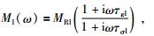
|
(1) |
其中ω为频率,相应的松弛应力模量和松弛时间为
|
(2) |
由于:

|
(3) |
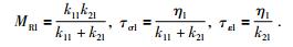
介质的应力和应变满足:
|
(4) |
令:

|
(5) |
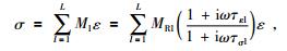
则介质的复应力模量为
|
(6) |
品质因子Q往往被定义为
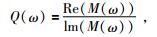
|
(7) |
因此有:
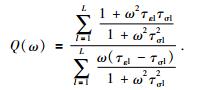
|
(8) |
由此得到了Q值与频率和松弛时间的关系式.若介质的Q值函数Q(ω)已经给定,Q值的松弛时间建模问题可以基于式(8)利用优化方法解决.目标函数可写为
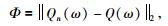
|
(9) |
其中Qn(ω)为估计的Q值函数,‖2‖为L2-范数.
下面将对基于优化方法的松弛时间建模的问题进行深入的研究.
2 恒定Q值的建模使式(9)达到极小值是典型的优化问题,可以利用L-M方法来解决.到目前为止,更多的研究集中在恒定Q值的建模问题,而且对恒定Q值的建模相对更简单一些,因此本文首先研究恒定Q值的建模.
与以前的一些研究中的做法类似(Blanch et al., 1995; Hesthom et al., 2006),首先将应力松弛时间τσl的倒数的对数均匀分布,然后求取使得式(9)达到极小值的应变松弛时间τεl.以Q=20为例,采用5个SLS进行建模,即L=5.建模的频率范围为2 Hz到25 Hz.应力松弛时间首先取为与Blanch文章(Blanch et al., 1995)中相同,如表 1所示.利用该文章中的τ方法得到的应变松弛时间作为初值.建模的结果如图 2所示,可以看到建模结果较好,最大相对误差为1.1%,平均相对误差为0.27%.
|
|
表 1 Q=20,频率范围2 Hz到25 Hz时的τσl (Blanch et al., 1995) Table 1 τσl that yields Q=20 between 2 Hz and 25 Hz (Blanch et al., 1995) |

|
图 2 Q=20,频率范围2 Hz到25 Hz时的建模结果,τσl与Blanch文章(Blanch et al., 1995)中相同 Figure 2 Optimal approximation for Q=20, the interested frequency range is from 2 Hz to 25 Hz, the values of τσl are same as that in the paper of Blanch et al (1995) |
利用τ方法得到的结果如图 3所示,最大相对误差为3%,平均相对误差为0.92%.可见利用L-M方法得到的结果精度更高.

|
图 3 Q=20,频率范围2 Hz到25 Hz时利用τ方法的建模结果 τσl与Blanch文章(Blanch et al., 1995)中相同. Figure 3 Approximation result for Q=20 with τ method, the interested frequency range is from 2 Hz to 25 Hz The values of τσl are same as that in the paper of Blanch et al (1995). |
在很多研究中都认为将应力松弛时间τσl的倒数的对数均匀分布可以得到较好的效果,但是其均匀分布的区间如何选取并没有人进行研究.在部分研究中,将建模的频率区间选为分布区间.在本例中,若将应力松弛时间τσl的倒数的对数均匀分布在2 Hz到25 Hz,得到的结果如图 4所示.最大相对误差为1.1%,平均相对误差为0.31%.建模结果与图 2中的结果接近.

|
图 4 Q=20,频率范围2 Hz到25 Hz时利用L-M方法的建模结果 τσl的倒数的对数均匀分布在2 Hz到25 Hz, L=5. Figure 4 Optimal approximation for Q=20, the interested frequency range is from 2 Hz to 25 Hz The reciprocals of τσl are distributed logarithmically over the frequency range of interest, L=5. |
若将分布区间扩大为[fmin/2, fmax×2], 其中fmin和fmax分别为建模频率区间的最小和最大频率,建模结果如图 5所示.最大相对误差为0.18%,平均相对误差为0.054%.与图 3、4相比,精度大大提高了.

|
图 5 Q=20,频率范围2 Hz到25 Hz时利用L-M方法的建模结果 τσl的倒数的对数均匀分布在[fmin/2, fmax×2], L=5. Figure 5 Optimal approximation for Q=20, the interested frequency range is from 2 Hz to 25 Hz The reciprocals of τσl are distributed logarithmically over [fmin/2, fmax×2], L=5. |
为研究增大分布区间是否总是可以改进建模精度,我们选取Q值更大的模型进行计算.若Q为100,建模区间为2 Hz到25 Hz,将τσl的倒数的对数均匀分布在[fmin/2, fmax×2]时建模结果如图 6所示.最大相对误差为0.18%,平均相对误差为0.049%.与前例类似,建模精度较高.如图 7,若分布区间选为[fmin, fmax],最大相对误差为0.95%,平均相对误差为0.28%,可见将分布区间选取为[fmin/2, fmax×2]大大提高了建模精度.另外,将图 6、7与图 3、4对比可以看到,当Q值较大时,同等条件下的建模精度稍高.

|
图 6 Q=100,频率范围2 Hz到25 Hz时的建模结果 τσl的倒数的对数均匀分布在[fmin/2, fmax×2], L=5. Figure 6 Optimal approximation for Q=100, the interested frequency range is from 2 Hz to 25 Hz The reciprocals of τσl are distributed logarithmically over [fmin/2, fmax×2], L=5. |

|
图 7 Q=100,频率范围2 Hz到25 Hz时的建模结果 τσl的倒数的对数均匀分布在[fmin, fmax], L=5. Figure 7 Optimal approximation for Q=100, the interested frequency range is from 2 Hz to 25 Hz The reciprocals of τσl are distributed logarithmically over [fmin, fmax], L=5. |
然而,进一步加大分布区间并不能得到更高的建模精度.若将分布区间增大为[fmin/10, fmax×10],建模结果如图 8所示.最大相对误差为0.43%,平均相对误差为0.15%,尽管建模精度仍然优于分布区间选为[fmin, fmax]时的结果,但是精度低于分布区间选为[fmin/2, fmax×2]时的结果.有此可见,将应力松弛时间τσl的倒数的对数均匀分布在一个大于建模频率区间的区间上可以得到更高的建模精度,但是分布区间的大小需合理.我们建议将分布区间选为最小频率的一半到最大频率的二倍.在本文后面的研究中,应力松弛时间τσl均如此选取.

|
图 8 Q=100,频率范围2 Hz到25 Hz时的建模结果 τσl的倒数的对数均匀分布在[fmin/10, fmax×10], L=5. Figure 8 Optimal approximation for Q=100, the interested frequency range is from 2 Hz to 25 Hz The reciprocals of τσl are distributed logarithmically over [fmin/10, fmax×10], L=5. |
可见将τσl的倒数的对数均匀分布在[fmin/2, fmax×2]可以得到较高的建模精度.下面应用本文中方法对实际场地数据进行建模.伍向阳等(1993)通过实验测得了砂岩的Q值,当砂岩含水量为0,即不含水时,其Q值约为13.2.利用本文方法对其进行建模,建模频率范围2~25 Hz,取L=5,将τσl的倒数的对数均匀分布在[fmin/2, fmax×2],结果如图 9所示.最大相对误差为0.2%,平均相对误差为0.059%,仍然保持较高的精度.王小杰和印兴耀(2011)对海上油田数据进行了分析,发现该场地含气层Q值大约为60.69,仍然采用本文方法对其进行建模,建模频率范围2~25 Hz,取L=5,将τσl的倒数的对数均匀分布在[fmin/2, fmax×2],结果如图 10所示.最大相对误差为0.16%,平均相对误差为0.049%,精度与前例接近.可见本文中方法适用于实际场地中恒定Q值的建模.

|
图 9 Q=13.2的不含水砂岩,频率范围2 Hz到25 Hz时的建模结果 τσl的倒数的对数均匀分布在[fmin/2, fmax×2], L=5. Figure 9 Optimal approximation for non aqueous sandstone that Q=13.2 The interested frequency range is from 2 Hz to 25 Hz, the reciprocals of τσl are distributed logarithmically over [fmin/2, fmax×2], L=5. |

|
图 10 Q=60.69的含气地层,频率范围2 Hz到25 Hz时的建模结果 τσl的倒数的对数均匀分布在[fmin/2, fmax×2], L=5. Figure 10 Optimal approximation for gas-bearing strata that Q=60.69 The interested frequency range is from 2 Hz to 25 Hz, the reciprocals of τσl are distributed logarithmically over [fmin/2, fmax×2], L=5. |
一些研究认为Q值是随频率变化的(Jeng et al., 1999;Rix and Meng, 2005).目前已有人基于广义Maxwell模型研究了随频率变化的Q值的建模问题.在本部分,我们将基于广义线性固体研究了随频率变化的Q值的建模问题.2005年,Rix和Meng通过实验得到了有机玻璃(PMMA)和改铸高岭土的阻尼比(Rix and Meng, 2005).有机玻璃的Q值随频率变化的趋势与函数类似,函数公式为
|
(10) |
当L=5时,建模结果如图 11所示.最大相对误差为0.16%,平均相对误差为0.049%.尽管此时Q值随频率变化,利用本文中方法的建模精度仍然很高.因此本文中方法同样适用于随频率变化的Q值的建模.

|
图 11 对近似于PMMA的Q值函数建模的结果 Q值函数由式(10)给出,L=5. Figure 11 Optimal approximation of the Q value corresponds to PMMA Q function is given by Eq. (10), L=5. |
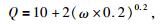
改铸高岭土的Q值随频率变化的趋势与函数类似,函数公式为
|
(11) |
当L=5时,建模结果如图 12所示.最大相对误差为5.3%,平均相对误差1.0%.建模误差远大于图 11中的结果.在我们的研究中发现,对于类似于式(11)中的随频率增大而减小的Q值的建模精度往往比其他情况更低.类似的情况也发生在基于广义Maxwell模型建模的过程中(Liu and Archuleta, 2006).

|
图 12 对近似于改铸高岭土的Q值函数建模的结果 Q值函数由式(11)给出,L=5. Figure 12 Optimal approximation of the Q value corresponds to remolded kaolin Q function is given by Eq. (11), L=5. |
若将SLS的个数增加5个,即L=10,建模结果如图 13所示.最大相对误差为0.28%,平均相对误差0.043%.此时建模精度有了显著的提高.因此,对于类似的情况,若建模精度较低,可以采用增加SLS个数的方法来提高精度.

|
图 13 对近似于改铸高岭土的Q值函数建模的结果 Q值函数由式(11)给出,L=10. Figure 13 Optimal approximation of the Q value corresponds to remolded kaolin Q function is given by Eq. (11), L=10. |
本文基于广义线性固体给出了一种Q值的松弛时间建模方法,这种方法适用于恒定Q值和随频率变化的Q值.通过对应力松弛时间选取的研究,发现当将应力松弛时间的倒数的对数均匀分布在最小频率的一半到最大频率的二倍区间内时建模精度最高,分布区间过大或过小都会导致建模误差增大,因此建议采用这种方法选取应力松弛时间.通过对实际场地的恒定Q值数据建模发现利用该方法可以得到较高的建模精度.通过分别对近似于有机玻璃和改铸高岭土的随频率变化的Q值函数进行建模发现本文中的方法同样适用于随频率变化Q值.对于一些随频率逐渐减小的Q值函数的建模精度相对较低,可以通过增加SLS个数来提高精度.本文中的研究对基于广义线性固体的时域波场模拟有一定意义.
致谢 感谢审稿专家提出的修改意见和编辑部的大力支持!| [] | An Y. 2015. Fracture prediction using prestack Q calculation and attenuation anisotropy[J]. Applied Geophysics, 12(3): 432–440. DOI:10.1007/s11770-015-0493-1 |
| [] | Asvadurov S, Knizhnerman L, Pabon J. 2004. Finite-difference modeling of viscoelastic materials with quality factors of arbitrary magnitude[J]. Geophysics, 69(3): 817–824. DOI:10.1190/1.1759468 |
| [] | Blanch J O, Robertsson J O A, Symes W W. 1995. Modeling of a constant-Q:Methodology and algorithm for an efficient and optimally inexpensive viscoelastic technique[J]. Geophysics, 60(1): 176–184. DOI:10.1190/1.1443744 |
| [] | Cai W T, Hu G Y, Fan T E, et al. 2014. Quality factor extraction by spectral simulation method[J]. Progress in Geophysics , 29(2): 642–649. DOI:10.6038/pg20140223 |
| [] | Carcione J M. 1992. Modeling anelastic singular surface waves in the earth[J]. Geophysics, 57(6): 781–792. DOI:10.1190/1.1443292 |
| [] | Day S M, Minster J B. 1984. Numerical simulation of attenuated wavefields using a Padé approximant method[J]. Geophysical Journal of International, 78(1): 105–118. DOI:10.1111/j.1365-246X.1984.tb06474.x |
| [] | Emmerich H, Korn M. 1987. Incorporation of attenuation into time-domain computations of seismic wave fields[J]. Geophysics, 52(9): 1252–1264. DOI:10.1190/1.1442386 |
| [] | Hesthom S, Ketcham S, Greenfield R, et al. 2006. Quick and accurate Q parameterization in viscoelastic wave modeling[J]. Geophysics, 71(5): T147–T150. DOI:10.1190/1.2329864 |
| [] | Jeng Y, Tsai J Y, Chen S T. 1999. An improved method of determining near-surface Q[J]. Geophysics, 64(5): 1608–1617. DOI:10.1190/1.1444665 |
| [] | Johnston D H, Toksöz M N, Timur A. 1979. Attenuation of seismic waves in dry and saturated rocks:Ⅱ. Mechanisms[J]. Geophysics, 44(4): 691–711. DOI:10.1190/1.1440970 |
| [] | Lagarias J C, Reeds J A, Wright M H, et al. 1998. Convergence properties of the Nelder-Mead simplex method in low dimensions[J]. SIAM Journal of Optimization, 9(1): 112–147. DOI:10.1137/S1052623496303470 |
| [] | Liu P C, Archuleta R J. 2006. Efficient modeling of Q for 3D numerical simulation of wave propagation[J]. Bulletin of the Seismological Society of America, 96(4A): 1352–1358. DOI:10.1785/0120050173 |
| [] | Rix G J, Meng J W. 2005. A non-resonance method for measuring dynamic soil properties[J]. Geotechnical Testing Journal, 28(1): 1–8. |
| [] | Wang X J, Yin X Y. 2011. Estimation of layer quality factors based on zero-phase wavelet[J]. Progress in Geophysics , 26(6): 2090–2098. DOI:10.3969/j.issn.1004-2903.2011.06.025 |
| [] | Wang Z J, Cao S Y, Zhang H R, et al. 2015. Estimation of quality factors by energy ratio method[J]. Applied Geophysics, 12(1): 86–92. DOI:10.1007/s11770-014-0471-7 |
| [] | Wu X Y, Zou Y, Chen Z A, et al. 1993. An experimental study of compressive wave velocity and Q value of sandstone and marble[J]. Progress in Geophysics , 8(4): 186–191. |
| [] | Xia J H, Miller R D, Park C B, et al. 2002. Determining Q of near-surface materials from Rayleigh waves[J]. Journal of Applied Geophysics, 51(2-4): 121–129. DOI:10.1016/S0926-9851(02)00228-8 |
| [] | Zhang K, Luo Y H, Xia J H, et al. 2011. Pseudospectral modeling and dispersion analysis of Rayleigh waves in viscoelastic media[J]. Soil Dynamics and Earthquake Engineering, 31(10): 1332–1337. DOI:10.1016/j.soildyn.2011.05.004 |
| [] | 蔡文涛, 胡光义, 范廷恩, 等. 2014. 谱模拟法提取地层品质因子[J]. 地球物理学进展, 29(2): 642–649. DOI:10.6038/pg20140223 |
| [] | 王小杰, 印兴耀. 2011. 基于零相位子波地层Q值估计[J]. 地球物理学进展, 26(6): 2090–2098. DOI:10.3969/j.issn.1004-2903.2011.06.025 |
| [] | 伍向阳, 邹勇, 陈祖安, 等. 1993. 砂岩和大理岩纵波速度及Q值实验研究[J]. 地球物理学进展, 8(4): 186–191. |