 2017, Vol. 32


2. 昆明南方地球物理技术开发有限公司, 昆明 650231
2. Kunming Southern Geophysical Technology Development, Inc, Kunming 650231, China
由于印度板块与欧亚大陆自50 Ma以来的连续碰撞, 导致了青藏高原的不断隆升.缝合区地壳增厚的同时,伴随着发生了地壳物质的侧向逃逸(Molnar and Tapponnier, 1975; Tapponnier and Molnar, 1977; Royden et al., 2008).云南地区地处青藏高原东南缘,这里是高原内部物质挤出的一个重要通道(Royden, 1996; Clark and Royden, 2000; Klemperer, 2006;Royden et al., 2008).受西侧印度板块在缅甸下方产生的向东俯冲作用,以及青藏高原向东南方向挤出的影响,导致该区岩石圈变形十分强烈.在云南南部地区,地表高程仅为500 m,而在西北部却达到了4000 m(如图 1).在700 km的水平距离内,地表高程竟发生如此剧烈变化实属罕见.另外,该区的构造运动十分强烈,地质构造十分复杂、地震活动频繁,自20世纪70年代以来,云南地区相继发生了大于7.0级强震共7次.如图 1所示,近南北向的大型走滑断裂:怒江断裂、澜沧江断裂、金沙江—红河断裂、丽江—小金河断裂、鲜水河—小江断裂,形成了该区的主要构造格局,并将该区分割成了滇东块体、川滇菱形块体、印支块体和滇缅泰块体.

|
图 1 (a) 云南地区的地形、地震分布(红色圆圈,从公元1500至2013年,震级范围6.0≤MS≤8.0)、主要的活动断裂(黑色细实线)和宽频台站(黑色三角形).F1-怒江断裂带; F2-澜沧江断裂带; F3-金沙江—红河断裂带; F4-丽江—小金河断裂带; F5-鲜水河—小江断裂带); Ⅰ-滇东块体; Ⅱ-川滇菱形块体; Ⅲ-印支块体; Ⅳ-滇缅泰块体.左上角的插图表示青藏高原东南缘平滑后的高程,其间隔为1000 m,红色矩形代表研究区域;(b)本研究中用到的震中分布图,震中距在28°~95°的事件用于提取P波接收函数,55°~150°的事件用于提取S波接收函数 Figure 1 (a)Topography, earthquake distribution of Yunnan and its adjacent (red circles, since the B.C. 1500 to 2013, 6.0≤MS≤8.0), major active faults (black thin solid lines) and broad-band stations (black triangles). Key to symbols: Faults: F1-Nujiang Fault; F2-Lancangjiang Fault; F3-Jinshajiang-Red river Fault; F4-Lijiang-Jinhe Fault; F5-Xianshuihe-Xiaojiang Fault. Tectonic units: Ⅰ-eastern Yunnan Block; Ⅱ-Sichuan-Yunnan diamond-shaped Block; Ⅲ-Indochina block; Ⅳ-Yunnan-Burma-Thailand Block. The inset in the top left corner: Contour of smoothened elevations of southeastern Tibet, with interval being 1000 m. The red rectangle on the inset map is showing the study region; (b)Locations of the earthquakes used in this study. Events with epicentral distance between 28° and 95° are used for computation of PRFs, while those events with epicentral distance between 55° and 150° are used for computation of SRFs |
岩石圈由地壳和上地幔盖层组成,其下是软流圈.在研究岩石圈构造演化的过程中,上地幔间断面(例如Moho、LAB)的深度及形态特征是最重要的参数之一,其主要特点是P波、S波在间断面上会发生速度变化.在地球动力学模型中,虽然岩石圏和软流圈边界(LAB)是一级分界面,但是在地震学意义上的地球模型中,它们仅是弱的分界特征(Dziewonski and Anderson, 1981; Kennett and Engdahl, 1991).宽角观测意味着传播路径的水平部分要大于竖向部分,这一技术探测地壳结构较为有效(Kind et al., 2012).地震层析成像技术(体波或面波)通常被用于研究上地幔间断面的结构特征(Kanamori and Press, 1970; Knopoff, 1972),它们对速度呈梯度变化的区域较为敏感,但对间断面的变化不敏感(Kind et al., 2012).另外,区域面波层析成像的横向分辨尺度为300~400km,竖向分辨尺度为30~50 km(Rychert and Shearer, 2009);虽然远震体波层析成像的横向分辨较高,但竖向分辨较差(McKenzie and Priestley, 2008; Priestley and Tilmann, 2009).由于这些原因,精确测定岩石圈的厚度仍然是一项困难的工作(Kind et al., 2012).
过去30年里,云南地区已经取得了几千公里的地壳测深剖面(阚荣举和林中洋,1986;张中杰等,2002;Zhang and Wang, 2009),还完成了面波反演(胡家富等, 2008, Yao et al., 2008, 2010)、接收函数反演(Hu et al., 2005;Li et al., 2008a;Wu and Zhang, 2011; Xu et al., 2013)、接收函数与面波联合反演(胡家富等, 2005; Bao et al., 2015; 郑晨等,2016)、远震P波走时层析成像(Li et al., 2008b;Lei et al., 2009), 以及大地电磁测深(Bai et al., 2010;李冉等, 2014).这些结果主要提供了云南地区的地壳结构信息,由于受当时的观测条件和分辨率限制,导致该地区的下岩石圈结构信息尚很缺乏.
Langston(1977, 1979)提出了震源等效假定, 并从长周期远震体波中分离出了接收函数, Owens等(1984)把这一方法扩展到了宽频带记录.在过去的30多年里,作为探测台站下方地壳、上地幔间断面结构的有效手段, 接收函数技术得到了快速发展(Kind et al., 2012).虽然P波接收函数探测地壳结构十分有效,由于Moho面的多次相可能污染了来自岩石圈底部的转换相,以致很少用它来探测LAB的深度,成功用P波接收函数获得LAB深度的例子仅限于一些特殊地区(Rychert et al., 2007).最近发展起来的S波技术主要分离界面上的S-to-P转换相,而这一转换相比入射S波提前到达台站,可以有效防止了与多次波的叠加(Yuan et al., 2006).
本文利用云南地区13个固定台站记录的三分量远震资料,分别反褶积出各台站下方的P、S波接收函数,并在叠加的P波接收函数里识别相关的转换相,判识来自LAB的转换相,以此确定岩石圈的厚度.将P波接收函数与S波接收函数的结果进行对比,以此验证用P波接收函数探测岩石圈厚度的可靠性,并对这两种方法的探测误差进行总结.
1 方法 1.1 接收函数技术当P波入射到一个分界面上时,一部分会转换成S波,称之为Ps转换波,而另一部分仍然以P波的形式传播.如图 2a所示,为了分离Ps转换波,三分量记录(ZNE)中的两个水平分量(NE)被旋转到径向(R)和切向(T);由于地震波不一定是垂直入射到地表,故径向(R)不一定垂直入射波方向,于是径向(R)和垂直向(Z)分量被旋转到射线坐标系(LQT)下,以保证Q、T分量垂直于入射波L.因而L分量主要包含P波(入射P波或Sp转换波),Q分量主要包含S波(入射S波或Ps转换波).对于均匀和各向同性介质而言,切向分量能量较弱而被抛弃.当远震P波入射到地表时,垂直分量的尾波很弱,介质响应近似为δ函数,这就是所谓的震源等效性(Langston, 1979).故把径向分量对垂直分量进行反褶积得到的时间序列称之为P波接收函数.经过反褶积后,最大限度地消除了直达P波的影响,因而径向分量接收函数主要以S波(这里指Ps波)为主.在实际处理过程中,为了压制直达P波,增强Ps波,常以L分量对Q分量作反褶积(Yuan et al., 1997).除了Ps相外,还存在地表与界面之间的多次波PpPs和PsPs+PpSs(如图 2b).一般而言,在P波接收函数里,Ps和PpPs相与入射波的极性相同,而PsPs+PpSs相与入射波的极性相反(如图 2c).

|
图 2 不同地震分量的旋转、地震转换相和接收函数波形 (a)入射波路径与不同的坐标系,南北分量(N)和东西分量(E)被旋转到径向(R)和切向(T),R指向事件震中,T垂直R (见小阴影图).联合Z分量,这些分量被投影到正交的L和Q方向.BAZ是地震事件后方位角,i是P波入射角;(b)Moho面P-to-S转换波;(c)地表记录的理论接收函数波形. Figure 2 Rotation scheme of the displacement components, converted seismic phases and receiver functions waveforms (a) Incident rays and different coordinate systems. The north (N) and east (E) components are rotated to the radial (R) and transversal (T) components, where R is pointing to the event epicenter and T is perpendicular to R (inset in the lower right corner). These two components are then projected onto the orthogonal L and Q components (both in the same vertical plain) with the help of the vertical (Z) component. BAZ is the back azimuth of the event-station pair with respect to the north direction. The angle i is the incidence angle of the incoming P-wave; (b) Schematic representation of converted P-to-S phases at the Moho; (c) Theoretical receiver function waveforms (standard notation) recorded at surface. |
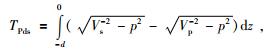
如图 2所示,若Moho面是最深的界面,地壳厚度H可以用直达P波与Ps转换波的时差tPs-tP表示为(Zhu and Kanamori, 2000)):

|
(1) |
其中,p是射线参数,Vp和Vs分别为P和S波的速度.类似地,延时tPpPs-tPs与地壳厚度H之间存在关系为

|
(2) |
而且有:

|
(3) |
从方程(1)和(2)我们可以得到:
|
(4) |
由于p是一个小量,故用Taylor展开下列式子,并取到二阶项有:
|
(5) |
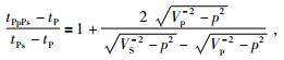
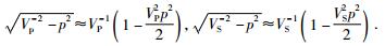
由于射线参数p与震中距有关,对于震中为67°时,p=0.057 s/km,若波速Vp=6.5 km/s,则VP2p2/2仅为0.07,而VS2p2/2则更小,它们均远远小于1,于是有:

|
(6) |
在式(6)中,若地壳波速比Vp/Vs在1.732~2.0之间,因而有:
|
(7) |
把方程(3)代入(7)则有:
|
(8) |
一般而言,Ps相较为清楚,其到时较为准确,而多次相PpPs和PsPs+PpSs为弱信号,其到时不易精确获得,通过方程(7)和(8)就可预测它们的达到时,可以帮助识别Moho面的多次相.
与P波入射的情况类似,当S波入射到界面上也会产生Sp转换波.然而,S波并不是先到达台站的震相,它常与P波的尾波同时到达,频率较低,且易受干扰.为了计算S波接收函数,通常是用Q分量对L分量作反褶积(Yuan et al., 1997).由于P波接收函数主要依据直达P波与Ps转换波之间的到时差来估算界面的厚度,其原理完全适用于S波接收函数.不过,Sp转换波先于直达S波到达台站,为了方便计算,实际处理中常把S波接收函数的时间轴和极性反转.另外,Sp转换相并不能在所有远震事件里观测到,有时可能仅发生于特定的入射角和转换深度(Li et al., 2007).
1.2 从时间域到深度域的转换技术由于接收函数是弱信号,故可以将很多个地震事件的接收函数进行叠加以达到增强信噪比的目的.然而,转换相的到时是入射角的函数,并受控于射线参数p.对于地表台站而言,要用叠加技术增强来自地下同一深度界面上的弱转换相,首先应保证这些相应该有相同的到时.若存在深度为d的界面,则该界面产生的Ps转换相的延时(Ps相与直达P波的到时差)为(Dueker and Sheehan, 1997, 1998):
|
(9) |
其中,Vp、Vs分别为P波和S波的速度,均为深度z的函数,p是射线参数.若给定速度模型,式(9)还表明:在深度为d的界面上产生的Ps转换相的延时随射线参数p而变化,这意味着界面深度d对应于多个Ps转换相的延时.由于射线参数p依赖于震中距,因而,在时间域里叠加接收函数时,必须将接收函数校正到同一参考震中距处.在校正过程中必须给定一个参考地球模型,以IASP91模型(Kennett and Engdahl, 1991)为例,在0~700 km的深度范围内,分别计算了射线参数p为8.98、6.40和4.70 s/(°)(相应的震中距分别为30°,67°和90°)时的Ps相与直达P波的延时(如图 3).如图 3所示,对于同一转换深度而言,Ps转换波与直达P波的延时随着震中距的减小(对应射线参数p增大)而增加.当射线参数p分别为8.98和4.70 s/(°)(相应的震中距分别为30°和90°)时,深度660 km的间断面产生的Ps相的到时差大于10 s.因此,为了用叠加技术来增强来自同一界面的转换相,需要在叠加之前先将地震事件校正到某一参考距离上(例如67°,相应的P波射线参数p=6.40 s/(°),而S波的射线参数则为p=12.07 s/(°).另外,利用上式还可进行时间域到深度域的转换,从而可在深度域里叠加接收函数.对于给定射线参数为p的接收函数,利用方程(9)计算出Ps相到时与深度的关系,并把接收函数的时间坐标映射成深度坐标,从而完成时间域到深度域的转换.

|
图 3 根据IASP91模型(Kennett and Engdahl, 1991)计算出的Ps相与转换深度的关系 b和c的射线参数分别为8.98、6.40和4.70 s/(°), 它们对应的震中距分别为30°、67°和90°.另外,曲线d的射线参数为12.07 s/(°), 相应于入射S波的震中距为67°. Figure 3 Relationship between conversion depth (in km) and time delay (in s) of the Ps phase computed from IASP91 model (Kennett and Engdahl, 1991) parameters for the curves a、b and c are 8.98, 6.40 and 4.70 s/(°), which correspond to epicentral distances 30°, 67° and 90°, respectively. Additionally, the ray parameter for curve d is 12.07 s/(°), which correspond to S wave incidence from distance 67°. |
本文收集了2007年1月1日到2009年5月13日之间云南区域地震台网13个台站记录的211个远震事件(如图 1b所示),这些地震事件的震级均在6.5级以上.震中距在28°~95°之间的事件用于提取P波接收函数,而震中距在55°~150°之间的事件用于提取S波接收函数.另外,所记录的远震事件大部分来自台网的东边,而来自台网西边的事件较少.
提取P波接收函数的计算过程如下:(1)截取P波之前10s,P波之后100s的时间信号,一个带宽为0.08~0.12 Hz的Butteworth滤波器用于消除高频信号;(2)三分量记录ENZ被旋转到ZRT坐标系下;(3)ZR分量被旋转到LQ方向;(4)在时间域里完成L分量对Q分量的反褶积(Ligorría and Ammon, 1999);(5)一个宽度为1 Hz的高斯滤波器用于去除高频噪声的影响.在本文中共获得了2002个P波接收函数,平均每个台站记录到了154个.
类似于P波接收函数的处理方法,S波接收函数的处理过程如下:(1)截取S波之前100s,S波之后20 s的时间信号,然后反转时间轴,以致Sp转换相具有正的到时,一个带宽为0.08~0.12 Hz的Butteworth滤波器用于消除高频信号;(2)三分量记录ENZ被旋转到ZRT坐标系下;(3)ZR分量被旋转到LQ方向;(4)在时间域里完成Q分量对L分量的反褶积(Ligorría and Ammon, 1999);(5)一个宽度为1 Hz的高斯滤波器用于去除高频噪声的影响.为了与P波接收函数保持一致,反转S波接收函数的极性,以保证来自Moho面的转换相SMp具有正极性.在本文中共获得了312条S波接收函数,平均每个台站记录到了24个.
为了分析P波接收函数中的Ps震相及其多次相,每一台站记录的所有接收函数被叠加成一道以增强信噪比.在叠加之前,根据IASP91模型(Kennett and Engdahl, 1991)将单道接收函数校正到了67°的参考震中距处,以保证同一界面的转换相具有相同的到时.如图 4给出了GEJ和TOH台的P波接收函数的单道及叠加道信号,可以清晰的分辨出GEJ和TOH台下方的Moho界面对应的PMs转换相与直达P波之间的时差分别为5.0 s和5.5 s,从图 3中查表知,P波接收函数给出这两个台站下方Moho界面的深度分别为42 km和44 km.按照方程(7)和(8),预测多次相PpPs的到时应该出现在15.0~26.0 s之间,而PsPs+PpSs应该出现在22.00~26.02 s之间.从图 4的叠加道读出GEJ台记录的PpPs和PsPs+PpSs的到时分别为15.8 s和21.9 s,TOH台记录的PpPs和PsPs+PpSs的到时分别为17.5 s和23.2 s,观测到时与预测关系较一致.另外,无论在单道接收函数还是叠加接收函数上,在PMs转换相后紧跟着一个负极性的转换相,这里称之为PLs相,它与直达P波之间的时差分别为8.5 s和9.0 s.在地球内部,速度随深度增加而增加的界面上产生的Ps相呈正极性,反之则呈负极性.既然PLs相已排除了Moho面多次相的可能性,它应该是一个新的转换相,这里解释为来自LAB的转换相,从图 3中查表知GEJ台和TOH台下方LAB的深度分别为67 km和75 km.

|
图 4 GEJ台(a)和TOH台(b)记录的单个P波接收函数和叠加道 单个接收函数按自然顺序排列,并且被校正到67°的参考震中距处,最上部的小图表示叠加道. Figure 4 The individual P-wave receiver functions and the stacked traces for (a) GEJ and (b) TOH stations The individual receiver functions are ordered randomly and moveout corrected to the reference distance of 67°, the top panel is the stacked receiver functions. |
由于S波在地幔中衰减较快,因此S波接收函数的频率比P波接收函数的低,导致了空间分辨率较低.有时它不能分辨精细的地壳结构,但比较适合于探测渐变的过渡区,例如LAB的情况(Li et al., 2007).为了比较P,S波接收函数得到的同一个台站下方的岩石圈厚度,如图 5给出了GEJ和TOH台的S波接收函数,单道接收函数在叠加之前被校正到了67°参考震中距处.这两个台站的叠加接收函数可以清晰的分辨出Moho界面与LAB界面对应的SMp和SLp转换相,而且具有较高的信噪比.然而,单道S波接收函数的一致性比P波接收函数差,尤其是GEJ台最明显.其原因可能是S波接收函数扫描的空间较大,地壳横向不均匀的影响不可忽略,另外,GEJ台处于小江断裂系和红河断裂系的交汇区(见图 1),深大断裂的影响也是一个因素.GEJ台和TOH台的SMp相对应的延时分别为7.4 s和6.8 s,从图 3查表知对应的深度分别为52 km和46 km.而SLp相对应的延时分别为13.5 s和11.1 s,查表知对应的深度分别为90 km和89 km.在这两个例子中,P、S波接收函数得到GEJ台下方的地壳厚度分别为42 km和52 km,LAB的深度分别为67 km和90 km;而TOH台下方的地壳厚度分别为44 km和46 km,LAB的深度分别75 km和89 km.由于GEJ台的单个S波接收函数相干性较差(见图 5a),导致S波得到的界面深度比P波接收函数得到的系统性偏大.对TOH而言,用P、S波接收函数得到的地壳厚度,LAB深度偏差较小.

|
图 5 GEJ台(a)和TOH台(b)记录的单个S波接收函数和叠加道 单个接收函数按自然顺序排列,并且被校正67°的参考震中距处,最上部的小图表示叠加道. Figure 5 The individual S-wave receiver functions and the stacked traces for (a) GEJ and (b) TOH stations The individual receiver functions are ordered randomly and moveout corrected to the reference distance of 67°, the top panel is the stacked receiver functions. |
为了对比分析这13个台的P、S波接收函数的探测结果,根据IASP91模型(Kennett and Engdahl, 1991)将接收函数先校正到了67°参考震中距处,利用方程(7)和(8)识别相关震相,确认来自Moho面的PMs相和来自LAB的PLs相.最后,利用方程(9)将叠加道信号转换到深度域,并读取来自Moho面的PMs相和来自LAB的PLs相的深度.与P波接收函数的处理方法类似,在每一个台站记录的S波接收函数叠加道上,取正极性的震相为来自Moho的SMp相,负极性的相为来自LAB界面的SLp相.为了方便查阅,我们将每个台站的叠加道里的转换相的到时及其深度汇编成表 1.根据台站的位置分布,我们将LUS、ERY、DAY、YUM和DOC五个台站叠加的P、S波接收函数投影到AB剖面上(如图 6),由PMs相得到地壳厚度在42~56 km之间,而SMp相得到的地壳厚度在45~54 km之间;由PLs相得到LAB的深度在74~84 km之间,而SLp相得到的LAB的深度在76~104 km之间.如图 7所示,我们将WAD、YOD、LIC、JIG、YUJ、TOH、GEJ和WES八个台站叠加的P、S波接收函数投影到CD剖面上,由PMs相得到地壳厚度在32~44 km之间,而SMp相得到的地壳厚度在41~52 km之间;由PLs相得到LAB深度在65~110 km之间,而SLp相得到的LAB的深度在66~135 km之间.
|
|
表 1 P、S波接收函数里各转换相的到时及对应的界面深度 Table 1 The arrival and depth of the converted phases on the P and the S receiver functions, respectively |

|
图 6 从P波接收函数(a)和S波接收函数(b)叠加道信号分别得到的地震剖面AB 接收函数顶部的大写字母代表台站名,台站和剖面位置见图 1. Figure 6 The seismic profile AB revealed by the stacked P receiver functions (a) and the stacked S receiver functions (b), respectively The upper letters on the top of the receiver functions denote the station code, the locations of the stations and the profile can be seen in the Fig. 1. |

|
图 7 从P波接收函数(a)和S波接收函数(b)叠加道信号分别得到的地震剖面CD 接收函数顶部的大写字母代表台站名,台站和剖面位置见图 1. Figure 7 The seismic profile CD revealed by the stacked P receiver functions (a) and the stacked S receiver functions (b), respectively The upper letters on the top of the receiver functions denote the station code, the locations of the stations and the profile can be seen in the Fig. 1. |
P波接收函数主要是分离界面产生的Ps相(Ammon et al., 1990; Ammon, 1991),而S波接收函数主要分离界面产生的Sp相(Yuan et al., 2006).对P波接收函数而言,Zhu和Kanamori (2000)使用H-k技术来估算地壳厚度,其原理是利用PMs相,以及多次振荡相PpPs和PpSs+PsPs的时差约束地壳厚度,优点是不依赖于参考地球模型,也不需要识别震相,特别适合计算机程序处理.然而,由于来自岩石圈底部的多次相几乎观测不到,故该方法不能用于探测LAB的深度.本文利用IASP91模型(Kennett and Engdahl, 1991)进行接收函数动校正、以及时间域到深度域的转换,虽然这一模型可能与云南地区存在差异,但这一偏差是系统性的,不会影响局部的异常特征.另外,P波走时层析成像(Lei et al., 2009;Li et al., 2008b)证实,云南地区的速度异常仅为1.0%~1.5%,由速度模型引起的深度估计偏差比较小,不影响对结果的评价.P波接收函数的结果表明,南部地区地壳较薄(见图 7),仅为32~35 km之间,北部地区地壳较厚(见图 6),可达到42~56 km之间,这与前人反演P波接收函数所得结果(Li et al., 2008a; Chen et al., 2013;Bao et al., 2015)以及贡山—贵阳的被动源地震观测剖面(Chen et al., 2015)较一致.S波接收函数的结果表明,在云南北部(见图 6),SMp相得到的地壳厚度在45~54 km之间,与PMs相得到的结果相比较,二者的偏差较小.然而,在云南南部地区(见图 7),由SMp相得到的地壳厚度在41~52 km之间,与P波接收函数的结果相比,呈现出系统性偏厚.从PMs相得到的结果与前人的结果一致,证实云南地区从南到北地壳呈增厚的变化趋势(Li et al., 2008a; Chen et al., 2013;Bao et al., 2015),而S波接收函数的结果并没有反映出这一变化趋势.其原因可能是S波接收函数的频率较低,对于较浅界面缺乏足够的分辨所致.
沿两个剖面的LAB深度表明(见图 6和7),云南大部分地区的岩石圈厚度仅为70~90 km.滇西地区大地热流值高达75~85 mW/m2(汪缉安等, 1990;Hu et al., 2000),该区已有的层析成像结果(Huang et al., 2002; Wang et al., 2003; Wang and Huangfu, 2004; Huang and Zhao, 2006; Li et al., 2008b; Lei et al., 2009)表明,滇西特提斯造山带下方的壳幔存在大尺度的低速区,一般认为这些低速区很可能是印度板块在缅甸下方向东俯冲,引起上幔热物质上涌所致(胡家富等,2005;2008;Lei et al., 2009).然而,受分辨率所限,这些结果并没有给出岩石圈的结构.Lei等(2014)利用青藏高原东缘的台阵记录的Pn走时数据,反演出云南地区Pn波的速度表明,上地幔顶部的低速区主要分布在红河断裂西侧,并沿丽江—小金河断裂向北东展布,这一低速区不但加热了岩石圈,而且剥离了岩石圈底部,导致滇西地区形成了较薄的岩石圈,这与本文的结果较一致.
本文分别从P、S波接收函数中提取的岩石圈厚度总体分布趋势较为一致,但局部存在较大差异.例如,GEJ台的S波接收函数得到的岩石圈厚度为90 km,而P波接收函数得到的岩石圈厚度为67 km,二者相差了23 km;WES台的S波接收函数得到的岩石圈厚度为135 km,而P波接收函数得到的岩石圈厚度为110 km,二者相差了25 km.这是因为来自LAB界面的PLs相面临两种情况:(1)岩石圈厚度较薄时,台站的PLs相较为清楚,此时从P和S波接收函数得到的结果相差较小;(2)当岩石圈厚度较大时(例如,大于100 km),尽管S波接收函数显示Sp相很清楚,但Sp相的转换点偏离台站较远,并不完全代表台站附近情况.另外,在P波接收函数里,来自LAB界面的PLs相可能与来自Moho界面的多次相出现在同一时间窗口内,导致误判PLs相,从而引起偏差.然而,已有的研究(Li et al., 2007)证实S波接收函数的测量误差大约为15 km,这一结论与本文的观测结果是一致的.
P波接收函数对界面较为敏感,由于频率较高,因而比S波接收函数的探测精度高.除了Moho面多次相的影响外,壳内界面产生的Ps相对识别PLs相也会产生影响,因此识别震相是关键.如图 6所示,DOC(东川)台的P波接收函叠加道上,在35 km附近出现了一个正极性的Ps相,根据前人的研究工作(Li et al., 2008a; Chen et al., 2013;Bao et al., 2015)和经过东川的被动源地震剖面(Chen et al., 2015),东川的地壳厚度为50~56 km.因此,我们认为这一个相不是来自Moho面的转换相,而是一个壳内的转换相.根据方程(7)和(8)预测它的多次相PpPs应该出现大约120 km左右,而负极性的PpSs+PsPs则应该在150 km附近.如图 6所示,这个预测结果与观测比较一致,因此我们认为出现在84 km附近的负极性相就是来自LAB的转换相PLs.另外,从S波接收函数得到的LAB深度为94 km,与P波接收函数得到的一致,证明对P波接收函数的震相识别是正确的.
4 结论 4.1岩石圏和软流圈边界(LAB)是地震学的弱界面,并不像Moho界面那样尖锐,探测其深度是一项很困难的工作.本文分离了云南区域地震台网13个台站记录的远震P、S波接收函数,在时间域里叠加后识别出来自Moho面的转换相和多次相,以及LAB界面的转换相,最后转换到深度域得到Moho面和LAB的深度.结果表明,P波接收函数得到的地壳厚度在32~56 km之间,S波接收函数得到的地壳厚度在41~54 km之间,S波接收函数得到地壳厚度系统地偏大8~9 km.P波接收函数得到的LAB深度在65~110 km之间,S波接收函数得到的LAB深度在66~135 km之间.一般而言,S波接收函数得到的LAB深度偏大15~20 km,最大偏差达到了25 km.
4.2P波接收函数的频率较高,而扫描的空间范围较S波小,它对界面深度变化最敏感,具有较高的分辨率.一般情况下,来自岩石圈底部的PLs相较弱,而且容易被Moho多次相污染.因此,P波接收函数只能适用于岩石圈较薄的情况,而且还必须仔细识别相关的震相.与此相反,由于Sp转换波比入射S波快,界面上的多次相与直达波是相互分离的,它不会受多次波的影响,因此特别适合探测岩石圈的底界面.不过,S波接收函数的频率较低,因而空间分辨率较P波接收函数的低.由于S波接收函数扫描的空间范围较大,若岩石圈厚度较大时,所得的岩石圈厚度并不完全代表台站下方的情况,而且会导致Sp相失去相干性,从而降低了探测精度.接收函数方法已经成为探测地壳上地幔的主要工具,P、S波接收函数处理的方法类似,但二者之间各有优缺点,实际应用中应相互补充.通过本文的对比分析,我们认为S波接收函数对浅部界面的分辨大致为35~40 km; 当岩石圈的厚度在120~200 km之间,由于Moho面多次相的干扰,P波接收函数可能无法确定PLs相.
致谢 感谢审稿专家提出的修改意见和编辑部的大力支持!| [] | Ammon C J. 1991. The isolation of receiver effects from teleseismic P wave forms[J]. Bulletin of the Seismological Society of America, 81(6): 2504–2510. |
| [] | Ammon C J, Randall G E, Zandt G. 1990. On the nonuniqueness of receiver function inversions[J]. Journal of Geophysical Research:Solid Earth, 95(B10): 15303–15318. DOI:10.1029/JB095iB10p15303 |
| [] | Bai D H, Unsworth M J, Meju M A, et al. 2010. Crustal deformation of the eastern Tibetan plateau revealed by magnetotelluric imaging[J]. Nature Geoscience, 3(5): 358–362. DOI:10.1038/ngeo830 |
| [] | Bao X W, Sun X X, Xu M J, et al. 2015. Two crustal low-velocity channels beneath SE Tibet revealed by joint inversion of Rayleigh wave dispersion and receiver functions[J]. Earth and Planetary Science Letters, 415: 16–24. DOI:10.1016/j.epsl.2015.01.020 |
| [] | Chen Y, Xu Y G, Xu T, et al. 2015. Magmatic underplating and crustal growth in the Emeishan Large Igneous Province, SW China, revealed by a passive seismic experiment[J]. Earth and Planetary Science Letters, 432: 103–114. DOI:10.1016/j.epsl.2015.09.048 |
| [] | Chen Y, Zhang Z J, Sun C Q, et al. 2013. Crustal anisotropy from Moho converted Ps wave splitting analysis and geodynamic implications beneath the eastern margin of Tibet and surrounding regions[J]. Gondwana Research, 24(3-4): 946–957. DOI:10.1016/j.gr.2012.04.003 |
| [] | Clark M K, Royden L H. 2000. Topographic ooze:Building the eastern margin of Tibet by lower crustal flow[J]. Geology, 28(8): 703–706. DOI:10.1130/0091-7613(2000)28<703:TOBTEM>2.0.CO;2 |
| [] | Dueker K G, Sheehan A F. 1997. Mantle discontinuity structure from midpoint stacks of converted P to S waves across the Yellowstone hotspot track[J]. Journal of Geophysical Research:Solid Earth, 102(B4): 8313–8327. DOI:10.1029/96JB03857 |
| [] | Dueker K G, Sheehan A F. 1998. Mantle discontinuity structure beneath the Colorado Rocky Mountains and High Plains[J]. Journal of Geophysical Research:Solid Earth, 103(B4): 7153–7169. DOI:10.1029/97JB03509 |
| [] | Dziewonski A M, Anderson D L. 1981. Preliminary reference Earth model[J]. Physics of the Earth and Planetary Interiors, 25(4): 297–356. DOI:10.1016/0031-9201(81)90046-7 |
| [] | Hu J F, Hu Y L, Xia J Y, et al. 2008. Crust-mantle velocity structure of S wave and dynamic process beneath Burma Arc and its adjacent regions[J]. Chinese Journal of Geophysics , 51(1): 140–148. DOI:10.3321/j.issn:0001-5733.2008.01.018 |
| [] | Hu J F, Su Y J, Zhu X G, et al. 2005. S-wave velocity and Poisson's ratio structure of crust in Yunnan and its implication[J]. Science in China Series D:Earth Sciences, 48(2): 210–218. DOI:10.1360/03yd0062 |
| [] | Hu J F, Zhu X G, Xia J Y, et al. 2005. Using surface wave and receiver function to jointly inverse the crust-mantle velocity structure in the West Yunnan area[J]. Chinese Journal of Geophysics , 48(5): 1069–1076. DOI:10.3321/j.issn:0001-5733.2005.05.013 |
| [] | Hu S B, He L J, Wang J Y. 2000. Heat flow in the continental area of China:A new data set[J]. Earth and Planetary Science Letters, 179(2): 407–419. DOI:10.1016/S0012-821X(00)00126-6 |
| [] | Huang J L, Zhao D P. 2006. High-resolution mantle tomography of China and surrounding regions[J]. Journal of Geophysical Research:Solid Earth, 111(B9): B09305. DOI:10.1029/2005JB004066 |
| [] | Huang J L, Zhao D P, Zheng S H. 2002. Lithospheric structure and its relationship to seismic and volcanic activity in southwest China[J]. Journal of Geophysical Research:Solid Earth, 107(B10): 2255. |
| [] | Kan R J, Lin Z Y. 1986. A preliminary study on crustal and upper mantle structures in Yunnan[J]. Earthquake Research in China , 2(4): 50–61. |
| [] | Kanamori H, Press F. 1970. How thick is the lithosphere?[J]. Nature, 226(5243): 330–331. DOI:10.1038/226330a0 |
| [] | Kennett B L N, Engdahl E R. 1991. Traveltimes for global earthquake location and phase identification[J]. Geophysical Journal International, 105(2): 429–465. DOI:10.1111/gji.1991.105.issue-2 |
| [] | Kind R, Yuan X H, Kumar P. 2012. Seismic receiver functions and the lithosphere-asthenosphere boundary[J]. Tectonophysics, 536-537: 25–43. DOI:10.1016/j.tecto.2012.03.005 |
| [] | Klemperer S L. 2006. Crustal flow in Tibet:Geophysical evidence for the physical state of Tibetan lithosphere, and inferred patterns of active flow[A].//Law R D, Searle P, Godin L eds. Channel Flow, Ductile Extrusion and Exhumation in Continental Collision Zones[M]. Geological Society, London, Special Publications, 268(1):39-70. |
| [] | Knopoff L. 1972. Observation and inversion of surface-wave dispersion[J]. Tectonophysics, 13(1-4): 497–519. DOI:10.1016/0040-1951(72)90035-2 |
| [] | Langston C A. 1977. Corvallis, Oregon, crustal and upper mantle receiver structure from teleseismic P and S waves[J]. Bulletin of the Seismological Society of America, 67(3): 713–724. |
| [] | Langston C A. 1979. Structure under Mount Rainier, Washington, inferred from teleseismic body waves[J]. Journal of Geophysical Research:Solid Earth, 84(B9): 4749–4762. DOI:10.1029/JB084iB09p04749 |
| [] | Lei J S, Li Y, Xie F R, et al. 2014. Pn anisotropic tomography and dynamics under eastern Tibetan plateau[J]. Journal of Geophysical Research:Solid Earth, 119(3): 2174–2198. DOI:10.1002/2013JB010847 |
| [] | Lei J S, Zhao D P, Su Y J. 2009. Insight into the origin of the Tengchong intraplate volcano and seismotectonics in southwest China from local and teleseismic data[J]. Journal of Geophysical Research:Solid Earth, 114(B5): B05302. DOI:10.1029/2008JB005881 |
| [] | Li C, van der Hilst R D, Meltzer A S, et al. 2008a. Subduction of the Indian lithosphere beneath the Tibetan Plateau and Burma[J]. Earth and Planetary Science Letters, 274(1-2): 157–168. DOI:10.1016/j.epsl.2008.07.016 |
| [] | Li R, Tang J, Dong Z Y, et al. 2014. Deep electrical conductivity structure of the southern area in Yunnan Province[J]. Chinese Journal of Geophysics , 57(4): 1111–1122. DOI:10.6038/cjg20140409 |
| [] | Li X Q, Yuan X H, Kind R. 2007. The lithosphere-asthenosphere boundary beneath the western United States[J]. Geophysical Journal International, 170(2): 700–710. DOI:10.1111/gji.2007.170.issue-2 |
| [] | Li Y H, Wu Q J, Zhang R Q, et al. 2008b. The crust and upper mantle structure beneath Yunnan from joint inversion of receiver functions and Rayleigh wave dispersion data[J]. Physics of the Earth and Planetary Interiors, 170(1-2): 134–146. DOI:10.1016/j.pepi.2008.08.006 |
| [] | Ligorría J P, Ammon C J. 1999. Iterative deconvolution and receiver-function estimation[J]. Bulletin of the Seismological Society of America, 89(5): 1395–1400. |
| [] | McKenzie D, Priestley K. 2008. The influence of lithospheric thickness variations on continental evolution[J]. Lithos, 102(1-2): 1–11. DOI:10.1016/j.lithos.2007.05.005 |
| [] | Molnar P, Tapponnier P. 1975. Cenozoic tectonics of Asia:Effects of a continental collision[J]. Science, 189(4201): 419–426. DOI:10.1126/science.189.4201.419 |
| [] | Owens T J, Zandt G, Taylor S R. 1984. Seismic evidence for an ancient rift beneath the Cumberland Plateau, Tennessee:A detailed analysis of broadband teleseismic P waveforms[J]. Journal of Geophysical Research:Solid Earth, 89(B9): 7783–7795. DOI:10.1029/JB089iB09p07783 |
| [] | Priestley K, Tilmann F. 2009. Relationship between the upper mantle high velocity seismic lid and the continental lithosphere[J]. Lithos, 109(1-2): 112–124. DOI:10.1016/j.lithos.2008.10.021 |
| [] | Royden L. 1996. Coupling and decoupling of crust and mantle in convergent Orogens:Implications for strain partitioning in the crust[J]. Journal of Geophysical Research:Solid Earth, 101(B8): 17679–17705. DOI:10.1029/96JB00951 |
| [] | Royden L H, Burchfiel B C, van der Hilst R D. 2008. The geological evolution of the Tibetan Plateau[J]. Science, 321(5892): 1054–1058. DOI:10.1126/science.1155371 |
| [] | Rychert C A, Rondenay S, Fischer K M. 2007. P-to-S and S-to-P imaging of a sharp lithosphere-asthenosphere boundary beneath eastern North America[J]. Journal of Geophysical Research:Solid Earth, 112(B8): B08314. |
| [] | Rychert C A, Shearer P M. 2009. A global view of the lithosphere-asthenosphere boundary[J]. Science, 324(5926): 495–498. DOI:10.1126/science.1169754 |
| [] | Tapponnier P, Molnar P. 1977. Active faulting and tectonics in China[J]. Journal of Geophysical Research, 82(20): 2905–2930. DOI:10.1029/JB082i020p02905 |
| [] | Wang C Y, Chan W W, Mooney W D. 2003. Three-dimensional velocity structure of crust and upper mantle in southwestern China and its tectonic implications[J]. Journal of Geophysical Research:Solid Earth, 108(B9): 2442. DOI:10.1029/2002JB001973 |
| [] | Wang C Y, Huangfu G. 2004. Crustal structure in Tengchong Volcano-Geothermal Area, western Yunnan, China[J]. Tectonophysics, 380(1-2): 69–87. DOI:10.1016/j.tecto.2003.12.001 |
| [] | Wang J A, Xu Q, Zhang W R. 1990. Heat flow data and some geologic-geothermal problems in Yunnan province[J]. Seismology and Geology , 12(4): 367–377. |
| [] | Wu J, Zhang Z J. 2011. Spatial distribution of seismic layer, crustal thickness, and Vp/Vs ratio in the Permian Emeishan Mantle Plume region[J]. Gondwana Research, 22(1): 127–139. DOI:10.1016/j.gr.2011.10.007 |
| [] | Xu X M, Ding Z F, Shi D N, et al. 2013. Receiver function analysis of crustal structure beneath the eastern Tibetan plateau[J]. Journal of Asian Earth Sciences, 73: 121–127. DOI:10.1016/j.jseaes.2013.04.018 |
| [] | Yao H J, Beghein C, van der Hilst R D. 2008. Surface wave array tomography in SE Tibet from ambient seismic noise and two-station analysis-Ⅱ. Crustal and upper-mantle structure[J]. Geophysical Journal International, 173(1): 205–219. DOI:10.1111/gji.2008.173.issue-1 |
| [] | Yao H J, van der Hilst R D, Montagner J P. 2010. Heterogeneity and anisotropy of the lithosphere of SE Tibet from surface wave array tomography[J]. Journal of Geophysical Research:Solid Earth, 115(B12): B12307. DOI:10.1029/2009JB007142 |
| [] | Yuan X H, Kind R, Li X Q, et al. 2006. The S receiver functions:Synthetics and data example[J]. Geophysical Journal International, 165(2): 555–564. DOI:10.1111/gji.2006.165.issue-2 |
| [] | Yuan X H, Ni J, Kind R, et al. 1997. Lithospheric and upper mantle structure of southern Tibet from a seismological passive source experiment[J]. Journal of Geophysical Research:Solid Earth, 102(B12): 27491–27500. DOI:10.1029/97JB02379 |
| [] | Zhang X, Wang Y H. 2009. Crustal and upper mantle velocity structure in Yunnan, Southwest China[J]. Tectonophysics, 471(3-4): 171–185. DOI:10.1016/j.tecto.2009.02.009 |
| [] | Zhang Z J, Teng J W, Li Y K, et al. 2004. Crustal structure of seismic velocity in southern Tibet and east-westward escape of the crustal material[J]. Science in China Series D:Earth Sciences, 47(6): 500–506. DOI:10.1360/03yd0518 |
| [] | Zheng C, Ding Z F, Song X D. 2016. Joint inversion of surface wave dispersion and receiver functions for crustal and uppermost mantle structure in Southeast Tibetan Plateau[J]. Chinese Journal of Geophysics , 59(9): 3223–3236. DOI:10.6038/cjg2016 |
| [] | Zhu L P, Kanamori H. 2000. Moho depth variation in southern California from teleseismic receiver functions[J]. Journal of Geophysical Research:Solid Earth, 105(B2): 2969–2980. DOI:10.1029/1999JB900322 |
| [] | 胡家富, 胡毅力, 夏静瑜, 等. 2008. 缅甸弧及邻区的壳幔S波速度结构与动力学过程[J]. 地球物理学报, 51(1): 140–148. DOI:10.3321/j.issn:0001-5733.2008.01.018 |
| [] | 胡家富, 朱雄关, 夏静瑜, 等. 2005. 利用面波和接收函数联合反演滇西地区壳幔速度结构[J]. 地球物理学报, 48(5): 1069–1076. DOI:10.3321/j.issn:0001-5733.2005.05.013 |
| [] | 阚荣举, 林中洋. 1986. 云南地壳上地幔构造的初步研究[J]. 中国地震, 2(4): 50–61. |
| [] | 李冉, 汤吉, 董泽义, 等. 2014. 云南南部地区深部电性结构特征研究[J]. 地球物理学报, 57(4): 1111–1122. DOI:10.6038/cjg20140409 |
| [] | 汪缉安, 徐青, 张文仁. 1990. 云南大地热流及地热地质问题[J]. 地震地质, 12(4): 367–377. |
| [] | 张中杰, 滕吉文, 李英康, 等. 2002. 藏南地壳速度结构与地壳物质东西向"逃逸"——以佩枯错-普莫雍错宽角反射剖面为例[J]. 中国科学(D辑), 32(10): 793–798. |
| [] | 郑晨, 丁志峰, 宋晓东. 2016. 利用面波频散与接收函数联合反演青藏高原东南缘地壳上地幔速度结构[J]. 地球物理学报, 59(9): 3223–3236. DOI:10.6038/cjg2016 |