 2021, Vol. 64


2. 东华理工大学核资源与环境国家重点实验室, 南昌 330013;
3. 核工业230研究所, 长沙 410011
2. State Key Laboratory of Nuclear Resources and Environment, East China University of Technology, Nanchang 330013, China;
3. No. 230 Research Institute of Nuclear Industry, Changsha 410011, China
磁法数据处理与解释是磁法勘探工作的核心环节,选取适当的方法技术是获得良好地质解释的关键.受磁化方向影响,磁异常往往与地质体分布之间存在一定偏差,直接进行异常解释难度较大.化极处理可以将感应磁化磁异常转换为垂直磁化异常,在一定程度上有利于异常的解释和推断.另外,许多数据处理方法建立在化极磁异常基础上,如归一化标准差(Cooper and Cowan, 2008)和Tilt-depth法(Salem et al., 2007).然而,当磁化角度变化较大,研究区位于低纬度,或工区存在强剩磁时,化极很难获得满意的效果.解析信号是磁异常解释的一类有效方法(Bastani and Pedersen, 2001; Srivastava and Agarwal, 2010; Cooper, 2015),二维解析信号不受磁化方向影响(Atchuta et al., 1981),三维磁异常解析信号受磁化方向影响较小,但仍不能无视斜磁化的影响(Huang and Guan, 1998; Li, 2006).Stavrev和Gerovsk(2000)在磁三分量和梯度张量基础上给出了R、L、E、Q四个模量转换量,并证实了这些转换量在三维中对磁化方向敏感度较小,二维中不受磁化方向影响.Verduzco等(2004)在tilt梯度的基础上提出了tilt梯度水平导数模,同样在二维磁异常处理中不受斜磁化影响,在三维中受磁化角度影响较小,也被广泛运用于磁异常识别中,不过该方法使用了磁异常二阶导数,易受噪声干扰影响,同时还会产生假异常.Wijns等(2005)提出了Theta map,这种方法可以有效识别低纬度磁异常的边界信息,但在中高纬度地区的应用效果较差.梯度全张量能够更好地描述场源的异常特征,近年来已被广泛应用于磁法数据处理中(Oruç, 2010; Beiki et al., 2011; 马国庆等,2012a),其中张量不变量(Schmidt and Clark, 2006)受磁化方向影响较小,但也依旧无法消除斜磁化的影响;归一化磁源强度(Beiki et al., 2012)同样是基于梯度张量的,该方法受磁化方向影响的程度更小,已被广泛重视与使用(Pilkington and Beiki, 2013; 饶椿锋等,2017).
磁异常的快速反演可以自动、快捷地获取场源位置信息,在磁异常解释中具有重要意义.欧拉反褶积(Thompson, 1982)是一种常用的方法,因其不需要先验信息、计算效率高而得到广泛的研究与应用(张季生等, 2011; Guo et al., 2014; 王林飞, 2016).Salem和Ravat(2003)基于欧拉反褶积和解析信号,提出了AN-EUL法,用于估计场源深度及构造指数,但该方法使用了三阶导数,更易受干扰影响.Salem等(2008)将tilt梯度和欧拉反褶积相结合提出了tilt-Euler法,该方法不仅削弱了斜磁化对反演结果的影响,还无需事先给定构造指数,推动了欧拉反褶积的实用化发展.Zhang等(2000)提出的张量欧拉反褶积在不提高导数阶次情况下,扩充了常规欧拉反褶积方程组个数,使得反演效果更佳,但该方法需要事先已知场源构造指数.马国庆等(2012b)提出了张量局部波数法的欧拉反褶积,实验显示该方法明显优于常规局部波数法.陈国强和马国庆(2016)在Theta图和欧拉反褶积方法基础上提出了Theta-Depth法,可有效反演场源的位置和深度,但这种方法需要事先对原始磁异常进行化极处理.
本文在方向tilt梯度(王彦国等, 2019)基础上,推导出了两个方向tilt梯度的不同方向导数,并同时将方向tilt梯度的导数与三个方向导数形式下的欧拉反褶积方程组相结合,推导出了方向tilt-Euler方程组,用于反演磁源参数.最后,通过模型实验和实例应用证实了该方法在斜磁化磁异常解释中的有效性及优越性.
1 基本原理 1.1 方向tilt梯度及其导数Tilt梯度(Miller and Singh, 1994)是一种可以均衡不同异常强度的位场数据处理方法,其理论公式为
|
(1) |
式中

方向tilt梯度(王彦国等,2019)的表达式为:
|
(2) |
|
(3) |
θx、θy分别为x,y方向上的方向tilt梯度.
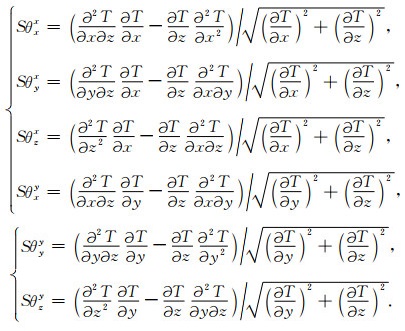
对公式(2)、(3)分别求x,y,z三个方向的导数,并对分母进行均方根处理,则得:
|
(4) |
公式(4)中的每一个表达式单位为nT·m-2或nT·km-2,与该式中使用的导数阶次相一致.王彦国等(2019)指出,利用方向tilt梯度水平导数模可以进行磁异常识别,其表达式为:
|
(5) |
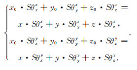
三维欧拉反褶积(Reid et al., 1990)的公式为:

|
(6) |
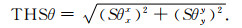
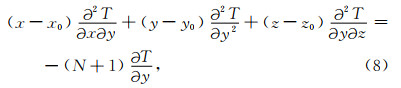
其中,x,y,z是观测点的坐标,x0,y0,z0是场源的位置坐标,N是构造指数.公式(6)对x,y,z三个方向求导,得:

|
(7) |
|
(8) |
|
(9) |
公式(9)乘以


|
(10) |
公式(9)乘以


|
(11) |
将公式(4)中的6个表达式代入公式(10)和(11),得:
|
(12) |
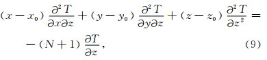
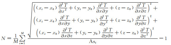
公式(12)即为方向tilt-Euler反演方程组.给定一个滑动计算窗口D(文中均选为5),通过求解超定方程组获得窗口下的场源位置反演解(x0, y0, z0).获得场源位置(x0, y0, z0)后,将公式(7)、(8)和(9)两边取平方,相加后取平方根,则得构造指数计算公式为:
|
(13) |
其中,解析信号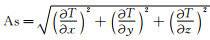
通过逐步滑动窗口直至完成全区的数据覆盖,则可以获得大量的反演解.然而,远离场源位置的反演解是不可靠的,需要进行有效的剔除处理.由于方向tilt梯度水平导数模THSθ极大值可作为磁性体的有效水平位置,因此可以剔除离THSθ极大值较远的反演解(文中删除了偏离THSθ极大值大于计算窗口宽度D的解),另外,还需要剔除反演深度小于0及构造指数大于4的反演解.
2 模型试验 2.1 单一模型首先设计一个磁化倾角为60°,磁化偏角为15°的单一长方体模型进行方法检验.模型体的长宽分别为20 km,上顶面埋深为1 km,下底面埋深为20 km,磁化强度为1 A·m-1.图 1为ΔT磁异常图,其中网格间距为0.5 km×0.5 km,黑色实线为模型体的理论边界位置.图 2为该模型磁异常方向tilt梯度的6个改进导数异常,可以看出,Sθxx突出的是地质体y方向的边界,Sθyx主要反映了长方体的四个角点,Sθzx异常主要分布在长方体y方向边界左右,边界上的异常值基本接近0值;Sθxy在一定程度上反映的也是y方向边界,Sθyy则明显突出了x方向上的边界,Sθzy异常则主要分布在场源边界附近,边界上异常值同样接近于0值,因此6个导数可以从不同方向和角度反映地质体的磁异常信息,有助于异常解释.图 3是方向tilt梯度水平导数模(公式(5))和方向tilt-Euler法(公式(12)、(13))计算结果.可以看出,方向tilt梯度水平导数模可以有效地识别场源边界,方向tilt-Euler法获得了较为准确的场源位置及构造指数.这表明基于方向tilt-Euler法可以进行斜磁化磁异常的有效解释工作.

|
图 1 单一长方体模型磁异常 Fig. 1 Magnetic anomaly of a single cuboid model |

|
图 2 单一长方体模型方向tilt梯度的改进导数 Fig. 2 The improved derivatives of the directional magnetic tilt-gradient of the single cuboid model (a) Sθxx; (b) Sθyx; (c) Sθzx; (d) Sθxy; (e) Sθyy; (f) Sθzy. |

|
图 3 单一长方体模型磁异常的方向tilt-Euler反演结果 (a) 方向tilt梯度水平导数模及反演解水平位置;(b) 深度反演解直方统计图;(c) 构造指数反演解直方统计图. Fig. 3 The inversion results of magnetic anomaly generated by the single cuboid model using the directional tilt-Euler method (a) The total horizontal derivative of the directional tilt-gradient and the horizontal locations of inversion solutions; (b) Histogram of the estimated depth solutions; (c) Histogram of the estimated structural index solutions. |
为了验证本文方法对复杂磁异常的处理能力,设计了一个由球体、岩脉体、正方棱柱体、薄板及长方体5个不同类型模型构成的组合模型,各模型体具有不同的磁化强度、磁化方向、埋深及水平尺度等参数,具体参数见表 1.图 4a为组合模型的原始磁异常,其中网格间距为0.1 km×0.1 km,可以看出,受磁化方向影响,磁异常与地质体并无明显对应关系.图 4b是tilt梯度的水平导数模,可以看出,该方法能够较好地识别出岩脉②的位置、长方体⑤的边界位置及正方棱柱体③部分边界,但是在球体①、岩脉②及薄板④附近存在着假异常.另外,极大值出现在薄板④边界的两侧.图 4c是方向tilt梯度水平导数模,可以看出,该方法可以很好地反映出所有模型体的位置,且不存在多余异常.
|
|
表 1 叠加模型参数 Table 1 The parameters of the multisource model |

|
图 4 组合模型磁异常及识别结果 (a) 理论磁异常;(b) Tilt梯度的水平导数模;(c) 方向tilt梯度的水平导数模. Fig. 4 Magnetic anomaly generated by multisource model and the recognized results (a) Forward magnetic anomaly; (b) The total horizontal derivative of the tilt gradient; (c) The total horizontal derivative of the directional tilt-gradient. |
图 5是tilt-Euler及方向tilt-Euler法反演解的平面分布图,从图中可以看出,tilt-Euler及方向tilt-Euler法都能够很好地反演出所有模型体的位置,但是tilt-Euler的反演解连续性及聚集度都没有方向tilt-Euler的强,且在球体下方(S1)、岩脉左上方(S2)及薄板右方(S3)存在三组虚假反演解.图 6和图 7分别是场源深度及构造指数的tilt-Euler法和方向tilt-Euler反演解直方分布图,可以看出,两者都很好地反演出了所有模型的深度及构造指数,不过方向tilt-Euler法精度更高,其深度及构造指数的均方误差分别为0.05 km和0.20,小于tilt-Euler法的0.09 km和0.32.且方向tilt-Euler法的反演解更接近正态分布,解的偏差也更小.另外,tilt-Euler法还获得了埋深分别为1.21 km,0.19 km和0.72 km的三个假源,这显然会给解释工作带来一定的干扰.

|
图 5 Tilt-Euler及方向tilt-Euler反演解平面位置 (a) Tilt-Euler; (b) 方向tilt-Euler. Fig. 5 The horizontal locations of inversion solutions by using the tilt-Euler and the directional tilt-Euler methods (a) The tilt-Euler; (b) The directional tilt-Euler. |

|
图 6 Tilt-Euler法反演结果 (a1), (b1), (c1), (d1), (e1) 分别是模型体1—5的深度反演解直方图;(a2), (b2), (c2), (d2), (e2) 分别是模型体1—5的构造指数反演解直方图;(f1), (g1), (h1) 是三个虚假源S1—S3的深度反演解直方图;(f2), (g2), (h2) 是三个虚假源S1—S3的构造指数反演解直方图. Fig. 6 Inversion results of the tilt-Euler method (a1), (b1), (c1), (d1), (e1) Histograms of the estimated depths of the models 1—5; (a2), (b2), (c2), (d2), (e2) Histograms of the estimated structural indices of the models 1—5; (f1), (g1), (h1) Histograms of the estimated depths of the three spurious sources; (f2), (g2), (h2) Histograms of the estimated structural indices of the three spurious sources. |

|
图 7 方向tilt-Euler法反演结果 (a1), (b1), (c1), (d1), (e1) 分别是模型体1—5的深度反演解直方图;(a2), (b2), (c2), (d2), (e2) 分别是模型体1-5的构造指数反演解直方图. Fig. 7 Inversion results of the directional tilt-Euler method (a1), (b1), (c1), (d1), (e1) Histograms of the estimated depths of the models 1—5; (a2), (b2), (c2), (d2), (e2) Histograms of the estimated structural indices of the models 1—5. |
为了了解噪声干扰对反演结果的影响,对叠加磁异常(图 4a)添加了0.5%的随机噪声(图 8a),图 8b和8c分别是tilt梯度及方向tilt梯度的水平导数模,不过对含噪磁数据进行了2倍点距的向上延拓处理.从图 8b和8c可以看出,tilt梯度的水平导数模更易受噪声影响,存在明显的数据波动,另外岩脉模型②左上侧的多余异常与岩脉异常基本连在一起,易被看作是有效异常;正方棱柱体③与长方体⑤之间存在一条明显的假异常.方向tilt梯度的水平导数模THSθ仍能够很好地识别出所有模型体的位置,不过岩脉和薄板的异常较为模糊.

|
图 8 含噪磁异常及识别结果 (a) 含0.5%噪声的磁异常;(b) 向上延拓2倍点距的tilt angle水平导数模;(c) 向上延拓2倍点距的方向tilt梯度水平导数模. Fig. 8 The noisy magnetic anomaly and its recognized results (a) Magnetic anomaly added by 0.5% random noise; (b) and (c) The total horizontal derivatives of the tilt gradient and the directional tilt gradient, but the data smoothed by upward continuation of 2 intervals. |
图 9a和9b分别是tilt-Euler及方向tilt-Euler反演解的平面位置展布图,对比可以看出,tilt-Euler反演解分布较为发散,尤其岩脉和正方棱柱体边界位置;在薄板体左边界,反演解呈现为两条带状分布,分别位于薄板边界的两侧;在岩脉左上侧、正方棱柱体与长方体之间均存在一个条带状分布反演解,这也易给解释工作带来麻烦.而方向tilt-Euler反演解具有更强的聚集度,反演解也更接近真实位置,且不存在虚假解.

|
图 9 含噪磁异常向上延拓2倍点距后的tilt-Euler及方向tilt-Euler反演解平面位置 (a) Tilt-Euler; (b) 方向tilt-Euler. Fig. 9 The horizontal locations of inversion solutions by using the tilt-Euler and the directional tilt-Euler methods for the noisy magnetic anomaly, but the data smooth by upward continuation of 2 intervals (a) The tilt-Euler; (b) The directional tilt-Euler. |
图 10与图 11分别是含噪声磁异常的tilt-Euler及方向tilt-Euler反演磁源深度及构造指数解的直方分布图,可以看出,方向tilt-Euler反演解的分布区间较小,解的均方差更小,也更接近于正态分布.方向tilt-Euler反演深度及构造指数的均方误差分别为0.11 km和0.43,也小于tilt-Euler的0.24 km和0.47,尤其深度反演精度是tilt-Euler的2倍.Tilt-Euler法还反演出了深度分别为0.05±0.06 km和0.35±0.31 km的两个假源.

|
图 10 含噪磁异常的tilt-Euler法反演结果 (a1), (b1), (c1), (d1), (e1) 分别是模型体1—5的深度反演解直方图;(a2), (b2), (c2), (d2), (e2) 分别是模型体1—5的构造指数反演解直方图;(f1), (g1)是两个虚假源S1—S2的深度反演解直方图;(f2), (g2)是两个虚假源S1—S2的构造指数反演解直方图. Fig. 10 Inversion results of the tilt-Euler method for the noisy magnetic anomaly (a1), (b1), (c1), (d1), (e1) Histograms of the estimated depths of the models 1—5; (a2), (b2), (c2), (d2), (e2) Histograms of the estimated structural indices of the models 1—5; (f1), (g1) Histograms of the estimated depths of the two spurious sources; (f2), (g2) Histograms of the estimated structural indices of the two spurious sources. |

|
图 11 含噪磁异常的方向tilt-Euler法反演结果 (a1), (b1), (c1), (d1), (e1) 分别是模型体1-5的深度反演解直方图;(a2), (b2), (c2), (d2), (e2) 分别是模型体1-5的构造指数反演解直方图. Fig. 11 Inversion results of the directional tilt-Euler method for the noisy magnetic anomaly (a1), (b1), (c1), (d1), (e1) Histograms of the estimated depths of the models 1-5; (a2), (b2), (c2), (d2), (e2) Histograms of the estimated structural indices of the models 1-5. |
该试验结果表明了方向tilt-Euler法相对于tilt-Euler法,具有反演解聚集度高、精度高、准确度高,及受噪声干扰影响小和无虚假解等优点.
3 实际资料应用为了检验实际资料应用效果,选取了内蒙古塔木素地区的航磁数据进行测试.图 12为研究区的地质简图,工区西北侧以火山岩为主,其他地区则主要是沉积岩分布,局部有火山岩出露,研究区内主构造为近NE向.图中红色实线为已知断裂构造、红色虚线为前人利用地震资料推断的构造,红色箭头方向为地震资料推断的构造倾向.

|
图 12 内蒙古塔木素地区地质图 Fig. 12 Geological map of Tamusu area in Inner Mongolia |
图 13a为塔木素地区航磁异常(网格间距1 km×1 km),研究区北部及东南地区以高磁异常为主,磁异常高低与磁性高低的地质体分布并无明显对应关系.图 13b、13c和13d分别是磁异常的解析信号、tilt梯度水平导数模和方向tilt梯度水平导数模.解析信号(图 13b)整体表现为西北高和中部及东南部低的异常特征,与地质图中的火山岩和沉积岩分布均有良好的对应性,中部及东南部还存在着局部高值区,可能是含有火山岩成分的沉积岩或隐伏火山岩引起的,但解析信号对弱信号的识别能力较差,异常细节特征无法清晰识别.Tilt梯度水平导数模(图 13c)获得了丰富的异常细节信息,异常圈闭走向与地质单元分布及断裂构造走向具有一定的相关性,但该方法的计算结果中存在虚假信息(王彦国等,2019).方向tilt梯度水平导数模同样获得了较为丰富的异常细节信息,看起来像是对解析信号(图 13b)细节特征的突出.另外,在沉积岩分布区内,断裂构造附近基本上都有方向tilt梯度水平总导数模的极大值响应,且这些极值异常恰位于断裂构造倾向方向.

|
图 13 塔木素航磁异常及不同方法的异常识别结果 (a) 航磁异常;(b) 解析信号振幅;(c) Tilt梯度水平导数模;(d) 方向tilt梯度水平导数模. Fig. 13 Aeromagnetic anomaly of Tamusu area and the recognized results using different methods (a) Aeromagnetic anomaly; (b) Analytic signal amplitude; (c) The total horizontal derivative of tilt gradient; (d) The total horizontal derivative of the directional tilt-gradient. |
图 14是tilt-Euler法和方向tilt-Euler法的反演结果.从整体上来看,两种方法计算得到的场源位置及构造指数均较为接近,反演解的水平位置基本上为条带状,反演深度值大多在0~2000 m之间,构造指数则主要分布在-0.6~1.4之间,尤其沉积岩分布区内的构造指数大部分在0值附近.这些信息表明了沉积岩分布区的磁异常主要是由断裂构造产生的.从反演效果来看,方向tilt-Euler法的反演解个数更多、聚集度更强、连续性更好,更能有效地追踪断裂构造的延伸.如图 14中箭头所指位置,方向tilt-Euler法反演解连续,条带状明显,而tilt-Euler法反演解较为发散、连续性较差.另外,可根据方向tilt梯度水平导数模和方向tilt-Euler法反演结果,推断隐伏断裂构造及地下磁性体分布,为研究该地区地下地质结构特征提供了一种依据.如图 14b、d中勾勒出了部分(隐伏)断裂带和一个隐伏岩体,其中断裂带①基本上是岩浆岩与沉积岩的界限断裂,应是东北向地表出露及前人推断断裂带在西南侧的延伸;断裂带②则将西南与东北侧断裂连接在一起;断裂带③推测是东侧断裂带的向西延伸;而断裂带④、⑤、⑥推测为隐伏构造带,这些断裂带在方向tilt梯度水平导数模(图 13d)及方向tilt-Euler(图 14b)都有着清晰的展示,而常规的tilt-Euler反演解(图 14a)偏少,连续性较差,不利于断裂带的精细划分.在圈定的隐伏岩体Ⅰ范围内,地表有花岗岩、闪长岩的零星分布,而解析信号(图 13b)和方向tilt梯度水平总梯度模(图 13d)在该区域存在大面积的强信号,方向tilt-Euler反演的深度较深及构造指数较大,故可推测地下存在大规模的隐伏岩体.

|
图 14 塔木素地区航磁数据tilt-Euler及方向tilt-Euler法反演结果 (a) Tilt-Euler法反演位置解;(b) 方向tilt-Euler法反演位置解;(c) Tilt-Euler反演构造指数解;(d) 方向tilt-Euler反演构造指数解. Fig. 14 The inversion results of the tilt-Euler method and the directional tilt-Euler method for aeromagnetic data of Tamusu area (a) The inversion locations of the tilt-Euler method; (b) The inversion locations of the directional tilt-Euler method; (c) The inversion structural indices of the tilt-Euler method; (d) The inversion structural indices of the directional tilt-Euler method. |
在方向tilt梯度基础上,推导出了方向tilt梯度的6个导数,构建了基于方向tilt梯度的欧拉反褶积(方向tilt-Euler法),用于三维磁异常解释工作.模型试验表明,相对于tilt梯度水平导数模来说,方向tilt梯度水平导数模可以更好地反映不同磁化方向的磁源位置,且不会产生多余异常;而方向tilt-Euler法反演解的连续性、汇聚度及精度也均高于tilt-Euler法的.在内蒙古塔木素地区航磁资料应用中,方向tilt梯度水平总梯度模及方向tilt-Euler法获得了丰富的异常信息和地下磁性体参数,反演信息揭示了沉积岩分布区内磁异常主要源自断裂构造,且解释结果与已知地质资料和地震解释结果吻合较好,同时反演结果也为地下磁性体分布特征研究提供了依据.
致谢 衷心感谢两位匿名评审专家为本文提供的宝贵建议.
Atchuta R D, Babu H V R, Narayan P V S. 1981. Interpretation of magnetic anomalies due to dikes; The complex gradient method. Geophysics, 46(11): 1572-1578. DOI:10.1190/1.1441164 |
Bastani M, Pedersen L B. 2001. Automatic interpretation of magnetic dike parameters using the analytical signal technique. Geophysics, 66(2): 551-561. DOI:10.1190/1.1444946 |
Beiki M, Pedersen L B, Nazi H. 2011. Interpretation of aeromagnetic data using eigenvector analysis of pseudogravity gradient tensor. Geophysics, 76(3): L1-L10. DOI:10.1190/1.3555343 |
Beiki M, Clark D A, Austin J R, et al. 2012. Estimating source location using normalized magnetic source strength calculated from magnetic gradient tensor data. Geophysics, 77(6): J23-J37. DOI:10.1190/geo2011-0437.1 |
Chen G Q, Ma G Q. 2016. Theta-Depth method for the interpretation of potential field data. Chinese Journal of Geophysics (in Chinese), 59(6): 2225-2231. DOI:10.6038/cjg20160625 |
Cooper G R J, Cowan D R. 2008. Edge enhancement of potential-field data using normalized statistics. Geophysics, 73(3): H1-H4. DOI:10.1190/1.2837309 |
Cooper G R J. 2015. Using the analytic signal amplitude to determine the location and depth of thin dikes from magnetic data. Geophysics, 80(1): J1-J6. DOI:10.1190/geo2014-0061.1 |
Guo C C, Xiong S Q, Xue D J, et al. 2014. Improved Euler method for the interpretation of potential data based on the ratio of the vertical first derivative to analytic signal. Applied Geophysics, 11(3): 331-339. DOI:10.1007/s11770-014-0442-4 |
Huang L P, Guan Z N. 1998. Discussion on "Magnetic interpretation using the 3-D analytic signal" by Walter R. Roest, Jacob Verhoef, and Mark Pilkington. Geophysics, 63(2): 667-670. DOI:10.1190/1.1444366 |
Li X. 2006. Understanding 3D analytic signal amplitude. Geophysics, 71(2): L13-L16. DOI:10.1190/1.2184367 |
Ma G Q, Li L L, Du X J. 2012a. Boundary detection and interpretation by magnetic gradient tensor data. Oil Geophysical Prospecting (in Chinese), 47(5): 815-821. |
Ma G Q, Du X J, Li L L. 2012b. Comparison of the tensor local wavenumber method with the conventional local wavenumber method for interpretation of total tensor data of potential fields. Chinese Journal of Geophysics (in Chinese), 55(7): 2450-2461. DOI:10.6038/j.issn.0001-5733.2012.07.029 |
Miller H G, Singh V. 1994. Potential field tilt-a new concept for location of potential field sources. Journal of Applied Geophysics, 32(2-3): 213-217. DOI:10.1016/0926-9851(94)90022-1 |
Oruç B. 2012. Location and depth estimation of point-dipole and line of dipoles using analytic signals of the magnetic gradient tensor and magnitude of vector components. Journal of Applied Geophysics, 70(1): 27-37. |
Pilkington M, Beiki M. 2013. Mitigating remanent magnetization effects in magnetic data using the normalized source strength. Geophysics, 78(3): J25-J32. DOI:10.1190/geo2012-0225.1 |
Rao C F, Yu P, Hu S F, et al. 2017. The 3D inversion of the normalized source strength data based on weighted model parameters. Geophysical Prospecting for Petroleum (in Chinese), 56(4): 599-606. |
Reid A B, Allsop J M, Granser H, et al. 1990. Magnetic interpretation in three dimensions using Euler deconvolution. Geophysics, 55(1): 80-91. DOI:10.1190/1.1442774 |
Salem A, Ravat D. 2003. A combined analytic signal and Euler method (AN-EUL) for automatic interpretation of magnetic data. Geophysics, 68(6): 1952-1961. DOI:10.1190/1.1635049 |
Salem A, Williams S E, Fairhead J D, et al. 2007. Tilt-depth method: A simple depth estimation method using first-order magnetic derivatives. The Leading Edge, 26(12): 1502-1505. DOI:10.1190/1.2821934 |
Salem A, Williams S, Fairhead D, et al. 2008. Interpretation of magnetic data using tilt-angle derivatives. Geophysics, 73(1): L1-L10. DOI:10.1190/1.2799992 |
Schmidt P W, Clark D A. 2006. The magnetic gradient tensor: Its properties and uses in source characterization. The leading Edge, 25(1): 75-78. DOI:10.1190/1.2164759 |
Srivastava S, Agarwal B N P. 2010. Inversion of the amplitude of the two-dimensional analytic signal of the magnetic anomaly by the particle swarm optimization technique. Geophysical Journal International, 182(2): 652-662. DOI:10.1111/j.1365-246X.2010.04631.x |
Stavrev P, Gerovska A. 2000. Magnetic field transforms with low sensitivity to the direction of source magnetization and high centricity. Geophysical Prospecting, 48(2): 317-340. DOI:10.1046/j.1365-2478.2000.00188.x |
Thompson D T. 1982. EULDPH: A new technique for making computer-assisted depth estimates from magnetic data. Geophysics, 47(1): 31-37. DOI:10.1190/1.1441278 |
Verduzco B, Fairhead J D, Green C M, et al. 2004. New insights into magnetic derivatives for structural mapping. The Leading Edge, 23(2): 116-119. DOI:10.1190/1.1651454 |
Wang L F, Guo C C, Xue D J, et al. 2016. Analytic signals of magnetic gradient tensor and their application to estimate source location. Progress in Geophysics (in Chinese), 31(3): 1164-1172. DOI:10.6038/pg20160333 |
Wang Y G, Luo X, Deng J Z, et al. 2019. 3D magnetic data interpretation based on improved tilt angle. Oil Geophysical Prospecting (in Chinese), 54(3): 685-691. |
Wijns C, Perez C, Kowalczyk P. 2005. Theta map: Edge detection in magnetic data. Geophysics, 70(4): L39-L43. DOI:10.1190/1.1988184 |
Zhang C Y, Mushayandebvu M F, Reid A B, et al. 2000. Euler deconvolution of gravity tensor gradient data. Geophysics, 65(2): 512-520. DOI:10.1190/1.1444745 |
Zhang J S, Gao R, Li Q S, et al. 2011. A combined Euler and analytic signal method for an inversion calculation of potential data. Chinese Journal of Geophysics (in Chinese), 54(6): 1634-1641. DOI:10.3969/j.issn.0001-5733.2011.06.023 |
陈国强, 马国庆. 2016. 位场数据解释的Theta-Depth法. 地球物理学报, 59(6): 2225-2231. DOI:10.6038/cjg20160625 |
马国庆, 李丽丽, 杜晓娟. 2012a. 磁张量数据的边界识别和解释方法. 石油地球物理勘探, 47(5): 815-821. |
马国庆, 杜晓娟, 李丽丽. 2012b. 解释位场全张量数据的张量局部波数法及其与常规局部波数法的比较. 地球物理学报, 55(7): 2450-2461. DOI:10.6038/j.issn.0001-5733.2012.07.029 |
饶椿锋, 于鹏, 胡书凡, 等. 2017. 基于加权模型参数的归一化磁源强度三维反演. 石油物探, 56(4): 599-606. DOI:10.3969/j.issn.1000-1441.2017.04.017 |
王林飞, 郭灿灿, 薛典军, 等. 2016. 磁梯度张量解析信号分析法及其在场源位置识别中的应用. 地球物理学进展, 31(3): 1164-1172. DOI:10.6038/pg20160333 |
王彦国, 罗潇, 邓居智, 等. 2019. 基于改进tilt梯度的三维磁异常解释技术. 石油地球勘探, 54(3): 685-691. |
张季生, 高锐, 李秋生, 等. 2011. 欧拉反褶积与解析信号相结合的位场反演方法. 地球物理学报, 54(6): 1634-1641. DOI:10.3969/j.issn.0001-5733.2011.06.023 |