 2020, Vol. 63


2013年11月17日09时04分55秒(UTC), 在南极斯科舍海域发生了一次MW7.8地震, 震中位置在南奥克尼群岛以北、南极板块与斯科舍板块之间(图 1)(下称“2013年南斯科舍海岭MW7.8地震”).南极板块相对于斯科舍板块以6~7mm·a-1的速度向东移动,使南斯科舍海岭转换带成为整个南极地区地震最活跃的区域(Ye et al., 2014).自1976年以来,MW4.9以上地震已经发生24次,多以走滑型震源机制为主,但也伴有其他类型.这说明斯科舍板块与南极板块的交界处应力环境并不均匀,构造也不简单.2013年发生的MW7.8地震是这一地带有地震记录以来最大的一次事件,其余震的空间分布以及USGS和GCMT的震源机制结果(表 1)表明,这次地震断层近东西走向,断层向南倾斜,倾角在44°~68°之间.地震破裂长度超过250 km (Ye et al., 2014), 明显高于同级地震的平均长度.其破裂持续时间也远大于基于标量地震矩估计的时间(Kanamori and Anderson, 1975).

|
图 1 2013年南斯科舍海岭MW7.8地震的构造与地震活动背景 红色六角形和海滩球分别表示主震震中位置和震源机制,红色圈代表余震.绿色六角形和海滩球分别表示2003年南斯科舍海岭MW7.6地震位置和震源机制.灰色五角星和海滩球分别表示1976年至今MW4.9以上历史地震的矩心位置和它们的震源机制.黄色实线表示海沟位置,黄色箭头表示移动方向 Fig. 1 Tectonic and seismicity settings of the 2013 MW7.8 South Scotia Ridge earthquake The red hexagram and beach-ball refer to the mainshock epicenter and focal mechanism solution, respectively, and the red circles are the aftershocks. The green hexagram and beach-ball are the epicenter and focal mechanism solution of the 2003 MW7.6 South Scotia Ridge earthquake, respectively. The gray stars and beach-balls are the centroid and focal mechanism solutions of the historical earthquakes above MW4.9 recorded since 1976, respectively. The yellow curves represent the trench. The yellow arrows indicate the movement directions. |
|
|
表 1 2013年斯科舍海MW7.8地震震源机制解 Table 1 Focal mechanism solutions of the 2013 MW7.8 South Scotia Ridge earthquake |
2013年南斯科舍海岭MW7.8地震矩心东侧约162 km处曾于2003年8月4日发生过一次具有类似震源机制的MW7.6地震(下称“2003年南斯科舍海岭MW7.6地震”).有学者使用W震相(一种在上地幔与地表之间传播的、类似于声学中回音(Whispering)的长周期波(Kanamori,1993)反演了这两次地震的矩心矩张量,用反投影技术和面波视震源时间函数分析了破裂的传播特征,并利用远场体波、面波以及可用的GPS静态位移反演确定了它们的滑动分布(Ye et al., 2014).结果表明2013年南斯科舍海岭MW7.8地震持续时间约120s,平均破裂速度2.5 km·s-1,造成了两个滑动凹凸体的破裂,而2003年南斯科舍海岭MW7.6地震主要的滑动凹凸体位于2013年地震的两个凹凸体之间.然而, 至今还没有这次地震震源机制时空变化的研究.
在国际上,单点的矩心矩张量反演已成为日常工作,例如,全球范围内的大地震发生后,哈佛大学很快用体波、面波以及地幔波反演并发布矩心矩张量解(GCMT)(Dziewonski et al., 1981; Ekström, 1989; Ekström et al., 2012);又如,美国地质调查局(USGS)通常利用W震相反演并发布矩心矩张量解(WCMT)(Kanamori and Rivera, 2008;Hayes et al., 2009; Duputel et al., 2012a).然而,多点的震源机制或矩张量反演一直以来都具有挑战性.有学者把整个观测波形看作多个子事件波形的延迟叠加,从而通过迭代过程逐次剥离子事件以达到反演多个子事件的震源机制的目的(Kikuchi and Kanamori, 1986;1991;Tocheport et al., 2006;Zahradník and Sokos, 2014),也有学者在固定子事件震源时间函数(三角形)的情况下,采用梯度类算法迭代反演各子事件矩张量解(Ekström, 1989; Tsai et al., 2005).还有人采用相邻算法采样器(Neighborhood Algorithm Sampler)(Sambridge, 1999),通过对每个子事件矩心可能出现的空间位置与时间延迟进行采样的方法反演矩心矩张量(Duputel et al., 2012b; Duputel and Rivera, 2017).我们曾经将子事件预设在沿断层走向的一条直线上,通过破裂速度控制子事件位置, 在给定子事件的震源时间函数的情况下反演了2008年汶川MW7.9地震震源机制的时空变化(张勇等,2009;Zhang et al., 2015).但是,无论如何,还没有一种通用的方法能够解决多点震源机制反演的问题.
广义台阵反投影技术是近年来研究大地震破裂时空过程的一种比较成熟的方法,它可以用来快速确定高频源的时空分布.自2004年苏门答腊MW9.2特大地震(Ishii et al., 2005)至今,已衍生诸多新技术(Ishii et al., 2007;Walker and Shearer, 2009; Meng et al., 2011; Yagi et al., 2012; Zhang et al., 2012;Yao et al., 2013; Xu et al., 2013; Wang and Mori, 2016; Qin and Yao, 2017;Yin et al., 2017;王晓欣等,2017;刘志鹏等,2018).我们也曾多次在一些地震中应用该技术研究其破裂时空特征(杜海林,2007;杜海林等,2009; Du et al., 2018;张旭等, 2019).视震源时间函数(Apparent source time function)也常常用来分析大地震破裂的复杂性,它不但可以揭示地震矩或能量释放随时间的起伏变化,还可以揭示破裂传播的方向变化(Lay and Wallace, 1995;Lanza et al., 1999;Duputel et al., 2012b; Park and Ishi, 2015;张旭,2016;张旭等,2019).
本文将介绍一种新的多点矩张量反演的方法并应用于2013年南斯科舍海岭MW7.8地震的多点矩张量解的反演.首先采用单点矩心矩张量反演方法,从W震相资料反演确定矩心矩张量解,然后利用广义台阵反投影方法获得高频源的时空分布,并利用PLD(Projected Landweber Deconvolution)方法(Berterto et al., 1997)从远场P波中提取依赖于方位的视震源时间函数,最后基于矩心矩张量解、高频源的时空分布以及视震源时间函数特征反演这次地震随时空变化的多点震源机制.这种方法利用矩心矩张量解、高频源的时空分布以及视震源时间函数的信息为约束,大大提高了多点震源机制解的稳定性和物理意义,且适用于非连续断层的复杂震源.
1 矩心矩张量大地震矩心矩张量反演可以使用体波、面波和地幔波(例如:GCMT),也可以使用W震相(例如:USGS-WCMT).由于W震相具有传播速度快、周期长、不易受浅层反折射震相干扰等优点(Kanamori,1993),在快速获取大地震、尤其特大地震的矩心矩张量解时具有一定优势,近年来广泛应用于震源机制快速求解甚至海啸预警(Duputel et al., 2012a).因此,在这项研究中我们利用W震相反演矩心矩张量.
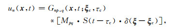
设τc为矩心时间,ξθ为矩心纬度,ξφ为矩心经度,ξh为矩心深度,则远场位移某个分量un(x, t)可表述为
|
(1) |
式中,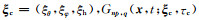

|
(2) |
这个线性系统因矩心位置的变化而变化.
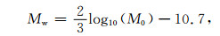
为了获取2013年南斯科舍海岭MW7.8地震的矩心矩张量,我们从全球台网(GSN)以及数字地震台网联合会(FDSN)数据网站下载了震中距范围在34°~86°的长周期地震记录和仪器响应数据,并根据背景噪声水平,以5°为方位间隔,挑选了23个台(图 2a)高质量的垂直向长周期记录(图 2b), 采用时间域剔除仪器响应的技术(Kanamori et al., 1999;Kanamori and Rivera, 2008)从观测数据中消除了仪器影响,并基于已有的研究经验(Kanamori and Rivera, 2008; Duputel et al., 2012a)将频率控制在0.0017~0.005 Hz范围内.首次搜索矩心时间时所使用的半持续时间τpre由标量地震矩加以估计(Kanamori and Anderson, 1975).在搜索矩心的水平位置时,在仪器震中位置的一定范围内构建网格,在每个格点求解震源机制,并将相应的合成波形与观测波形进行对比,波形匹配最佳的格点即为矩心的水平位置.矩心的水平位置确定后,再利用在不同深度计算的格林函数(Wang, 1999)逐一搜索,寻找观测资料和合成资料之间的残差达到最小的深度.需要说明的是,在矩张量反演时各向同性部分被约束为0.矩震级的计算则统一采用Kanamori等(Kanamori,1977)给出的如下公式:
|
(3) |

|
图 2 本研究中使用的地震台站分布及其长周期波形记录 (a)台站分布.红色六角星为主震震中,三角形为台站; (b)去除仪器响应并经0.0017~0.005 Hz带通滤波的垂直向记录.红色直线表示初至时刻,蓝色圆点表明W震相截止时间. Fig. 2 Distribution of the seismic stations with long-period recordings used in this study (a) Distribution of the stations. Red hexagram is the mainshock epicenter, and yellow triangles are the stations; (b) Vertical components of the long-period recordings after instrument response was removed and being filtered with a frequency band of 0.0017~0.005 Hz. The red vertical line shows the initial times of the W-phases while the blue dots indicate the ends. |
式(3)中,M0为标量地震矩,单位:dyne·cm.
图 3展示了2013年南斯科舍海岭MW7.8地震矩心矩张量反演过程与结果.尽管震源时间函数的初始半持续时间为18s,但最终搜索的结果为49 s (图 3a).仪器震中在60.37°S,46.58°W,深度为7.9 km,而矩心空间搜索得到的矩心水平位置为60.18°S、44.50°W,矩心深度约19 km(图 3b,3c).同时可以看到,从仪器震中位置得到的矩张量解也不同于最终反演得到矩心矩张量解(图 3d).反演结果表明,整个地震释放标量地震矩4.71×10²⁰N·m,相应的矩震级为MW7.75, 其中双力偶成分占比88%(图 3d).表 2列出了矩心位置和矩张量解参数,并与GCMT的相应参数进行了比较.比较发现,我们的位置在GCMT矩心位置的东北,矩心深度略浅,但矩张量解非常相似.与USGS、Ye等(Ye et al., 2014)以及GFZ的最佳双力偶解的比较展示于表 1.尽管已经发布的结果之间存在一定差异,但可以确定,2013年南斯科舍海岭MW7.8地震以走向近正东的断层的左旋走滑为主,倾角在44°至66°之间.GCMT和我们的矩张量解中都存在很强的非双力偶成分,这可能是由多个不同震源机制的子事件叠加所致.

|
图 3 矩心矩张量反演过程与结果 (a)二次失配函数值随矩心时间的变化轨迹(蓝色)以及最终采纳的震源时间函数(背景三角形).红色六角星和红色圆圈表示矩心时间预估值和最后采纳值对应的点; (b)二次失配函数值随矩心水平位置的变化.红色六角星和黑色五角星分别表示震中位置和矩心位置; (c)均方根残差随矩心深度的变化; (d)震中位置(PDE)和矩心位置对应的矩张量解(CMT). Fig. 3 The inversion of centroid moment tensor and the inverted results (a) The variation trace (blue) of the quadratic misfits with centroid times and the final source time function (background triangle). Red hexagonal star and dot refer to the predicted centroid time and final value, respectively; (b) The variation of the quadratic misfits with horizontal locations of the centroid. Red hexagonal and black stars indicate the locations of instrumental epicenter and centroid, respectively; (c) The variation of the RMS residuals with the centroid depth; (d) Centroid moment tensor solutions obtained at the instrumental epicenter(PDE) and centroid(CMT), respectively. |
|
|
表 2 与GCMT矩心矩张量解对比 Table 2 Comparison of our result with the global centroid moment tensor solution |
利用得到的矩心矩张量解计算的合成波形与观测波形的比较展示于图 4.我们把23个台站观测波形和合成波形连接起来进行比较,发现二者的均方根误差为2.06×10⁻⁷m·s-1,相关系数为0.89(图 4).

|
图 4 观测波形与合成波形的比较 红色圆点表示每个台站资料的起始点.台站和分向名展示在图顶部. Fig. 4 Comparison of the synthetic and observed data Red dots indicate the beginnings of the data from various stations and channels presented at top. |
视震源时间函数不仅携带着地震能量随时间变化的信息,而且还携带着破裂的方向性信息,因此得到广泛的关注和应用(Duputel et al., 2012b;Park and Ishi, 2015;张旭,2016;张旭等,2019).截至目前,已经有很多提取视震源时间函数的具体技术(Mori and Hartzell, 1990; Radulian and Popa, 1996;许力生等, 1999, 2002; Venkataraman et al., 2002),但Bertero(Berterto et al., 1997)提出的PLD方法,因为其独特的优势被广泛采用.这种方法把时间域里的褶积转化为频率域中的点积,大大提高了计算效率;同时在时间域添加物理约束,克服了频率域添加约束的困难.在前面的研究中,我们已经对这种方法进行过详细介绍并多次应用(张勇,2008;张旭,2016;张旭等,2019).概而言之,首先给定一个简单的震源时间函数(多为三角形函数),并通过傅里叶变换得到震源谱


|
(4) |
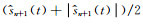
式(4)中,τ是松弛因子,其取值一般为


提取视震源时间函数的地震记录均来自全球地震台网.依据记录的信噪比、台站的空间分布以及观测地震图和合成地震图的拟合情况,最终选择了23个台站(图 5).提取视震源时间函数时,截取直达P波120 s(前10 s,后110 s),以GCMT的矩心矩张量参数计算相应的格林函数,依据波形复杂性与持续时间采用了0.01~0.05 Hz的频率范围(Lanza et al., 1999;Chen and Xu, 2000),并根据经验设定最大持续时间110 s.经过200次的迭代,最后获得如图 5a所示的视震源时间函数.可以看出这些视震源时间函数彼此之间具有相似性,但也随着台站的方位具有规律性变化.这不仅表明震源破裂的复杂性,也表明破裂具有明显的破裂优势方向.

|
图 5 依赖于台站方位的视震源时间函数分析 (a)视震源时间函数.横轴为时间,纵轴为台站方位,颜色表示峰值的相对时间,六角形表示峰值位置,红色曲线为优势破裂方向的最佳拟合,蓝色倒三角为优势方向,红色三角表示反方向; (b)台站分布.颜色含义与(a)中相同,粗虚线表示破裂优势方向,震中位置即矩张量解所在位置; (c)矩率函数(MRF:Moment Rate Function)的极坐标系展示.颜色为归一化的矩率,用不同色彩填充的圆圈既展示其峰值时刻,也表示台站方位. Fig. 5 Analysis of the azimuth-dependant apparent source time functions (ASTFs) (a) ASTFs. Horizontal axis shows time while vertical axis shows azimuths of stations, where color indicates relative times, hexagonal star refers to location of the peak, red curve exhibits the best fit for optimal rupture direction, inversed blue triangle indicates the optimal direction and red normal triangle shows opposite direction of the rupture; (b) Station distribution. The color has the same meaning as that in (a), dashed wide line indicates the optimal direction, epicenter is at the location of the beach-ball showing focal mechanism solution; (c) Display of the ASTFs in polo-coordinate frame. Normalized moment rate is presented in color, peak times are shown with circles filled with various color showing the azimuth. |
为了获得总体的破裂优势方位,我们利用各台站视震源时间函数的最大峰值时间τp以及台站相对于震中的离源角ih,基于Haskell模型(Lay and Wallace, 1995; Park and Ishii, 2015),通过公式
|
(5) |
进行了最小二乘拟合,得到最优破裂方位角φr=96°.上式中,a和b为拟合参数,φ为台站相对于震中的方位角.为了揭示依赖于方位的破裂复杂性的更多细节,我们将视震源时间函数投影到以时间为径向、台站方位角为切向的极坐标平面(图 5).除总体的破裂优势方向和地震矩的分段释放特征外,我们还可以看到更多地震矩率的时空复杂性.为了突显震源复杂性的总体认识,我们计算了所有台站的平均视震源时间函数(如图 6).可以看到,地震刚开始时能量释放率较低,但很快快速爬升,到60 s左右,能量释放率再次进入低谷,约80 s左右能量释放率达到最大,随后急速下行直到地震结束.总体上地震过程以60 s为界限分为前后两个阶段.但是,前60 s的视震源时间函数还呈现出两个峰,分别在23 s和44 s左右.

|
图 6 平均视震源时间函数 Fig. 6 The average of apparent source time functions |
图 7展示了不同台站得到的视震源时间函数、观测资料以及用视震源时间函数计算的合成资料.注意到,虽然个别台站(SBA)的观测资料和合成资料的拟合并不理想,相关系数为0.77,但总体上二者的匹配都很好,相关系数都在0.9以上.

|
图 7 不同台站的视震源时间函数(填充部分)以及用视震源时间函数合成的理论地震图与观测地震图的比较 Fig. 7 The apparent source time functions (ASTFs) retrieved from various stations (color-filled) and the comparison of the observed data (black) with the synthesized data (red) using the ASTFs |
我们采用的广义台阵技术是聚束能量技术(Ishii et al., 2005, 2007;杜海林等,2009).如果用u′j表示滤波后的原始波形记录,Aj表示振幅归一化因子,δt′j为观测走时与理论走时之差,wj为权重因子,则走时校正后的记录可表示为
|
(6) |
进一步,M个台站构成的台阵的聚束可定义为
|
(7) |
那么,在时间t1~t2之间的能量E为
|
(8) |
如果无需对聚束进行非线性处理,则N=1.
根据宽频带地震台在全球的分布, 针对非洲、澳洲和美洲等台站相对密集的区域, 通过考察地震记录走时校正后波形的相关度,我们最终从非洲大陆的133个台站中挑选了81个(图 8a).这些台站震中距范围为62.05°~89.01°,方位角在57.70°~107.44°之间,构成一个以W07CR台为中心、孔径达6428 km的台阵.尽管台阵的孔径非常大,但经走时校正(张喆等,2019)后首个10 s时窗的波形相关系数仍能达到0.92(图 9).根据地震记录的幅频特性(图 2)(张喆等,2019),我们选取0.3~2 Hz的信号作为反投影的观测数据.反投影时采用的积分时窗宽度为10 s, 滑动步长为0.5 s,数据总长为120 s,投影范围为59.5°S—61.5°S、47.2°W—40.0°W,网格大小为0.01°×0.01°,并采用AK135模型计算理论走时(Kennett et al., 1995).

|
图 8 台站与震中 (a)台阵相对于震中的位置;(b)台站分布. Fig. 8 Stations and epicenter (a) Seismic array with respect to the epicenter; (b) Stations comprising the array. |

|
图 9 P波初至到时校正 蓝色直线表示参考台P波初至时刻,红色波形为聚束波形. (a)校正前各台站波形与聚束波形平均相关度仅为0.13; (b)校正后相关度提高至0.92. Fig. 9 Calibration of the P arrival times The P arrival time at the reference station is shown with the vertical blue line, and the beamed recording is in red while others are in black. (a) Before the calibration, the correlation coefficient is only 0.13 on average between recording individuals and the beam; (b) After the calibration, the average of the correlation coefficients is up to 0.92. |
通过计算每个时间窗的聚束能量得到如图 10所示的110 s时间段内的相关系数(图 10a)、振幅比(图 10b)、聚束能量(图 10c)以及以及它们的点积γ-函数(图 10d)的相对大小(参见:杜海林等,2009;张喆等,2019),并基于γ-函数,我们以峰值的5%作为阈值,确定此次地震高频源的持续时间为100.5 s (图 10d).可以清楚地看到,高频能量具有至少5次峰值,分别出现在13 s、30 s、51 s、64 s和84 s.其中,图 11展示了震源过程中6个时间点聚束能量的空间分布.可以看出,这次地震明显是一次自西向东的单侧破裂.

|
图 10 有效持续时间的确定 (a)聚束波形与参考波形的相关系数;(b)聚束波形与参考波形的振幅比;(c)聚束能量;(d) γ函数.γ值降至最大值的5%时对应的时间为100.5 s. Fig. 10 Determination of the effective duration time Correlation coefficient between the beamed wavelet and the referenced one; (b) Amplitude ratio of the beamed wavelet to the referenced one; (c) Radiation energy; (d) Criterion function γ. The effective duration time 100.5 s is defined as the γ drops to 5% of the maximal amplitude here. |

|
图 11 不同时窗内聚束能量的空间分布.五角星表示破裂起始点,红色圆圈表示瞬时能量最大点 Fig. 11 Spatial distribution of the beam energy within various time windows, where red stars refer to the initial points and the red dots denote the points of the maximal energy within the windows |
将每个时间窗内能量的最大位置投影到径向为距离、切向为方位的极坐标系中,并利用最小二乘方法拟合,我们得到优势破裂方向为94°,能量最高点的方位为97°.同时得到最大破裂距离约311 km,能量最大点位置距离初始破裂点178 km(图 12a).将各时间窗内能量最大点的位置投影到以初始破裂点为坐标原点、以时间为横轴、以距离为纵轴的直角坐标系中,通过最小二乘法求得平均破裂速度为2.78 km·s-1(图 12b).同时可以看到,破裂过程是复杂的,破裂速度多次发生了变化.
基于高频能量的释放过程(高频震源时间函数),可以把这次地震过程分为5个阶段或5次子事(图 13a).我们将这些子事件的空间位置、能量最大点的时间和位置以及破裂速度和优势破裂方向展示于图 13b.再次发现,高频能量的释放过程与低频能量的释放过程并不相同(Du et al., 2018).

|
图 12 高频源参数的估计 (a)高频源在以径向为距离、切向为方位的极坐标系中的展示.最远破裂点距离起始破裂点311 km,最小二乘拟合表明平均破裂方位为94°;能量最大点距离起始点178 km, 破裂方位为97°; (b)高频源在以时间为横轴、距离为纵轴的直角坐标系中的展示.最小二乘拟合表明平均破裂速度为2.78 km·s-1,能量最大点之前的平均破裂速度也为2.78 km·s-1. Fig. 12 Estimation of the parameters of high-frequency sources (a) Display of the high-frequency sources in the poly coordinate frame in which distances are in radial direction while azimuths are in tangential direction. The farthest source is estimated to be 311 km from the initial point. The least-squared fit resulted in an average rupture azimuth of 94°. The maximal energy release occurred 178 km away from the initial point, and this location is at azimuth of 97°to the initial point; (b) Display of the high-frequency sources in the Cartesian coordinate frame in which horizontal axis presents time while vertical axis shows distances. The least-squared fit produced an average rupture velocity of 2.78 km·s-1, which was consistent with the average rupture velocity before the maximum energy release. |

|
图 13 基于高频源的时空特征辨识的5次子事件 (a)时间特征;(b)空间分布. Fig. 13 Identification of 5 subevents based on the spatiotemporal distribution of the high-frequency sources (a) Temporal feature; (b) Spatial distribution. |
与单点的矩心矩张量反演相比, 多点的矩张量反演采用观测资料约束下震源机制解逐渐拆分的策略,以避免未知数过多导致无物理意义的结果.具体而言,首先,考虑到W震相中低频成分占主导地位,缺失震源机制变化对地震信号的贡献,我们用体波代替W震相,适度提高观测资料的频率上限;然后,将矩心矩张量解拆分成两个或三个子事件的矩张量解.因此,多点矩张量反演问题变为如下联立求解的问题:

|
(9) |
将上式改写成矩阵形式
|
(10) |
式(10)中,λ和μ是用来调节资料方程与拆分方程之间的相对权重,I为对角线元素为1的单位矩阵.求解方程(10)有多种方法,但我们习惯于使用共轭梯度法,因为它不需要为系数矩阵求逆且便于添加约束.方程(9)和(10)仅适合于将一个事件拆分成两个子事件的情形,对于将一个事件拆分成3个或多个子事件的情形,只需对方程进行调整即可.但是,需要特别说明的是,随着子事件的增加反演结果会逐渐失去物理意义且反演结果不稳定.
在进行多点矩张量反演时采用的台站分布与进行矩心矩张量反演时完全相同,但为了使观测资料携带一定量的震源机制变化响应,我们采用了那23个台的垂直分量P波数据,波形数据的时窗均为[tp, tp+200 s](tp为P波到时),并将频带范围调整至0.002~0.01 Hz.另外,在反演时不但考虑了平均视震源时间函数揭示的地震矩率随时间的变化特征,而且还考虑了高频源的时空分布.根据平均视震源时间函数,将地震整体事件分为三个子事件,其矩率峰值分别出现在23 s、44 s与81 s,其中第一次与第二次子事件峰值比较接近且重叠较多,所以把这两次子事件合并为子事件A,第三次暂且定义为子事件B(图 6).
我们曾尝试在反演子事件地震矩张量的同时确定其矩心位置,但由于待解参数的增加导致反演不稳定.因此,我们不得不针对具体情况依据高频源的时空特征以及平均视震源时间函数时间特征,在反演震源机制的同时,选择性地确定矩心时间、矩心位置以及半持续时间.
综合考虑平均视震源时间函数与高频源的时空特征,将事件A的空间位置设置为子事件Ⅰ和Ⅱ的峰值点的中间位置,矩心时间定为34 s(23 s与44 s的均值).将事件B的位置设为子事件Ⅲ、Ⅳ和Ⅴ的峰值点的平均位置,矩心时间为81 s.
同样基于平均视震源时间函数与高频源的时空特征,设置事件A和B的半持续时间范围为[5 s, 34 s]以及[5 s, 29 s],并通过求
|
(11) |
的最小值来确定半持续时间τhA和τhB.上式中,Uobs和Usyn代表观测向量和合成向量.
图 14阐释了矩心矩张量分解为子事件A和B的过程.当χ达到最小时,τhA和τhB分别为28 s和20 s, 得到的震源机制解如表 3所示,标量地震矩分别为4.218×10²⁰N·m和2.519×10²⁰N·m,对应的矩震级为MW7.71和MW7.58.

|
图 14 子事件A、B的半持续时间与矩率时间函数的确定 (a)二次失配值随子事件A、B半持续时间的变化.当A和B的半持续时间分别为28 s和20 s时,失配值达到最小; (b)子事件A和B的矩率时间函数,红色和蓝色直线表示矩心时间. Fig. 14 Determination of the half-duration times and the moment rate time functions of subevents A and B (a) Variation of the quadratic misfits with the half-duration times of subevents A and B. The misfits reached the minimum as the half-duration times of subevents A and B are 28 s and 20 s, respectively; (b) The moment rate time functions of subevents A and B, where the red and blue lines indicate centroid times. |
|
|
表 3 双力偶解 Table 3 Double-couple solutions |
为了进一步拆分子事件A和B,将资料的频率上限提高至0.012 Hz.首先将子事件A拆分为子事件Ⅰ和Ⅱ.根据高频源的分布将二者的矩心位置设定为60.40°S/45.93°W与60.46°S/43.26°W.根据平均视震源时间函数将矩心时间设置23 s与44 s.为了反演结果的稳定性,反演过程需要在约束事件B的震源机制不变的条件下进行.这个约束类似于Kikuchi等(Kikuchi and Kanamori, 1991)从原始记录中逐渐剥离子事件的技术.事件Ⅰ和Ⅱ半持续时间通过2维搜索来确定.事件I的搜索范围为[5 s,23 s],事件Ⅱ的搜索范围为[5 s, 34 s].反演结果如图 15所示,半持续时间分别为21 s和17 s, 标量地震矩分别为2.585×10²⁰N·m和1.890×10²⁰N·m,对应的矩震级为MW7.57和MW7.48.

|
图 15 子事件Ⅰ、Ⅱ的半持续时间与矩率时间函数的确定(其他说明,请参看图 14) Fig. 15 Determination of the half-duration times and the moment rate time functions of subevents A and B (Also see Fig. 14 for other information) |
根据高频源的震源时间函数(图 13a)以及视震源时间函数(图 5a),除子事件Ⅰ和Ⅱ外,还可以看到子事件Ⅲ、Ⅳ和Ⅴ,因此采用与上面类似的技术将事件B进行了拆分.拆分的结果表明(图 16),事件Ⅲ半持续时间为6 s,标量地震矩为1.791×10¹⁹N·m,对应的矩震级为MW6.80;事件Ⅳ的半持续时间为16 s,标量地震矩为2.239×10²⁰N·m,对应的矩震级为MW7.53;事件Ⅴ的半持续时间为8 s,标量地震矩为4.701×10¹⁹N·m,对应的矩震级为MW7.08.

|
图 16 五次子事件的震源机制与震源时间函数 (a)子事件的空间位置及其震源机制解; (b)子事件的时间范围及其震源时间函数. Fig. 16 Focal mechanism solutions and source time functions of the five subevents (a) Spatial distribution and focal mechanism solutions of the subevents; (b) Time windows and source time functions of the subevents. |
需要特别说明的是, 尽管高频源震源时间函数以及视震源时间函数表明子事件B可以拆分为子事件Ⅲ、Ⅳ和Ⅴ,但是从平均视震源时间函数无法得知子事件Ⅲ和Ⅴ的矩心时间.考虑到矩心时间对远场长周期位移波形的影响比半持续时间更明显(Duputel et al., 2012a),所以在固定子事件Ⅳ的矩心时间等于子事件B的峰值时间,并仿照Duptel et al.(Duptel and Rivera, 2017)的做法给定子事件Ⅲ、Ⅳ和Ⅴ的半持续时间为10 s的情况下,首先对子事件Ⅲ和Ⅴ的矩心时间进行滑动步长为1 s的试错搜索.结果发现,当这两个矩心时间分别为65 s和102 s时,观测资料和合成资料的相关性达到最高.然后,固定这三个子事件的矩心时间,分别在时间范围[2 s,10 s]、[5 s,29 s]和[2 s,8 s]内进行三维搜索确定半持续时间.结果表明,6 s、16 s和8 s分别为子事件Ⅲ、Ⅳ和Ⅴ的最优半持续时间.
为了阐释多点源矩张量反演的必要性和合理性,我们利用单点源(矩心)和多点源矩张量反演结果分别计算的合成地震图与观测地震图进行了对比.如图 17所示,GCMT矩心矩张量解能够使0.002~0.01 Hz频带范围内的合成地震图和观测地震图的相关系数和均方根误差达到0.66和2.34×10⁻⁷m·s-1,能够使0.002~0.012 Hz频带范围内的相关系数和均方根误差达到0.61和2.83×10⁻⁷m·s-1.如果采用我们得到的WCMT矩心矩张量解,这四个数依次为0.67,2.07×10-7m·s-1, 0.60和2.73×10⁻⁷m·s-1.但是,5个子事件的矩张量解能够使0.002~0.012 Hz频带范围内的合成地震图和观测地震图的整体相关系数和均方根误差达到0.93和1.26×10⁻⁷m·s-1.

|
图 17 观测资料与合成资料的比较 (a) GCMT解对0.002~0.01 Hz观测资料的解释;(b) GCMT解对0.002~0.012 Hz观测资料的解释;(c)WCMT解对0.002~0.01 Hz观测资料的解释;(d)WCMT解对0.002~0.012 Hz观测资料的解释; (e)5个子事件的震源机制解对0.002~0.12 Hz的观测资料的解释. Fig. 17 Comparison between the observed and synthesized data (a) Frequency band of the data is 0.002~0.01 Hz and the focal mechanism solution used to synthesize data is GCMT. (b) Frequency band: 0.002~0.012 Hz; focal mechanism solution: GCMT. (c) Frequency band: 0.002~0.01 Hz; focal mechanism solution: WCMT. (d) Frequency band: 0.002~0.012 Hz; focal mechanism solution: WCMT. (e) Frequency band: 0.002~0.012 Hz; focal mechanism solution: solutions of the five subevents. |
2013年南斯科舍海岭MW7.8地震已经有多个震源机制反演结果(表 1,表 3).这些结果表明这个地震的走向在90°至103°方位,倾角在44°与66°之间,滑动角在-1°到-14°之间.我们的单点震源机制反演显示(表 3),断层走向104°,倾角54°,滑动角8°,与上述结果非常近似,一致表明这是一次左旋走滑为主的事件.除震源机制外,全球矩心矩张量解(表 2)还发布了矩心的位置.二者相比,我们得到的矩心位置偏东北56.8 km, 矩心深度相差5 km左右,GCMT给出的矩心位置处在南奥克尼岛的正下方,而我们的WCMT解的矩心则处于靠近海沟较浅的位置.另外,我们得到的剪切成分占88%,略低于全球矩心矩张量解给出的93%.
5.2 视震源时间函数长周期面波(瑞利波和勒夫波)视震源时间函数(Ye et al., 2014)显示2013年南斯科舍海岭MW7.8地震的持续时间在120s与125s之间,破裂长度245 km左右,破裂速度约2.5 km·s-1,优势破裂方位为98°.从依赖于方位的视震源时间函数可以辨认出两次子事件.为了揭示更多的破裂复杂性,我们选择了频率较高(0.01~0.05 Hz)的直达P波.正如所料,我们得到的视震源时间函数展示了更多的复杂性,从依赖于方位的震源时间函数至少可以分辨出3次子事件或者更多.平均地讲,破裂的优势方位在96°,破裂持续时间约110 s.
5.3 高频源的时空变化有学者已经分别利用分布在澳洲的33个宽频带台和北美(拉丁美洲)的59个宽频带地震台的记录对这次地震的高频(0.5 Hz~2.0 Hz)源进行了反投影成像(Ye et al., 2014).得到的两个结果均表明这是一次向东传播的单侧破裂,破裂速度在2~3 km·s-1之间,然而高频源时间函数明显不同,能量的空间分布也截然不同.根据Ye等(Ye et al., 2014)的结果, 破裂持续时间为120 s,破裂长度约250 km.在我们的研究中采用的是选自非洲的81个宽频带台站构成的台阵.根据我们的计算分析,这些台站构成的台阵响应优于澳洲和拉丁美洲的台站构成的台阵(图 18).事实上,非洲台阵数据的反投影可以直接把高频源确定在余震分布的海沟带,而无需海沟带的强制约束(Ye et al., 2014).我们的反投影结果表明,这次地震持续时间100.5 s,破裂尺度311 km,优势破裂方位94°,平均破裂速度2.78 km·s-1.高频源震源时间函数清楚地揭示出5次子事件,能量峰值点分别出现在13 s、30 s、51 s、64 s和84 s,各子事件的平均破裂速度分为别0.6 km·s-1、2.6 km·s-1、2.3 km·s-1、2.8 km·s-1和3 km·s-1.

|
图 18 频率为2 Hz时台阵响应的比较 (a)美洲台阵;(b)澳洲台阵;(c)非洲台阵.上面子图展示了震中相对于台阵的位置. Fig. 18 Comparison of the array response functions at frequency of 2 Hz (a) Americas; (b) Australia; (c) Africa. Note: the above subplots exhibit locations of the arrays with respective to the epicenter. |
截至目前,还没有关于这次地震的震源机制随时间或者空间变化的研究.本研究借助于高频源的时空分布特征以及直达P波视震源时间函数特征,将2013年南斯科舍海岭MW7.8地震拆分成5次子事件,反演得到了它们的震源机制解,揭示了这次地震的震源机制随时间和空间的变化(表 3,图 13,图 16).与此同时,我们还采用早期使用的方法(张勇等,2009)检验了这5次子事件的反演结果.如图 19所示,沿断层总体走向的一条直线上等间隔离散11个点源后得到的震源时间函数与平均视震源时间函数,以及本研究得到的5次子事件的震源时间函数都具有很好的一致性,11个点源与5次子事件对应时间段内的5个震源机制解也非常相似.

|
图 19 震源机制反演结果的对比 (a)平均视震源时间函数;(b)本研究反演得到的震源时间函数;(c)利用张勇等方法(张勇等,2009)反演得到的震源时间函数;(d)第一行为本研究得到的5次子事件的震源机制,第二行为利用张勇等的方法得到的对应时段的震源机制. Fig. 19 Comparison of the focal mechanism results inverted (a) The average of the ASTFs; (b) The source time function inverted in this study; (c) The source time function inverted using the technique proposed by Zhang et al.(Zhang et al., 2009); (d) On the first row are the focal mechanism solutions of the five subevents inverted in this study, and on the second row are those of the time windows corresponding to the five subevents inverted by the technique proposed by Zhang et al. (Zhang et al., 2009). |
根据我们的反演结果,这次地震断层走向的变化范围在81°至105°之间,倾角在46°至86°之间,滑动角在-17°至13°之间.第三次和第五次事件较小,半持续时间分别仅为6 s和8s.释放能量最多的是第一次子事件,相当于MW7.57.2013年南斯科舍海岭MW7.8地震震源机制的时空变化在一定程度上反映了当地的构造和应力的非均匀性,也是对当地历史地震具有多种震源机制的事实的有力支持.
5.5 特殊的第四次子事件根据已有的研究(Ye et al., 2014),2003年南斯科舍海岭MW7.6地震主要的滑动凹凸体位于2013年地震的两个凹凸体之间,即沿海沟42°W—44°W之间.这个范围与2013年地震的第四次子事件的位置相对应.根据他们的结果,2003年地震断层走向在101°至103°之间,倾角在36°至63°之间,滑动角在-23°与-32°之间.根据我们的结果(表 3),这里的断层走向98°,倾角46°,滑动角13°.两个结果在走向和倾角方面的差别似乎可以接受,但滑动角的差别比较明显,二者相差36°,甚至55°.这意味着当地的应力状态在10年尺度上是变化的,似乎正是这种变化的应力状态在10年的时间里积累了几乎相当的能量,形成了两个震级相当的地震.
6 总结借助于2013年南斯科舍海岭MW7.8地震,我们提出并验证了一种反演大地震随时空变化的震源机制的新方法(多点源震源机制反演方法).新方法主要由两步组成,一是整个事件的矩心矩张量解的反演,二是观测波形资料约束下的矩张量解的逐级拆分.第一步,利用可以将地震整体事件作为点源的低频波形记录反演确定事件的矩心矩张量解(矩心位置,半持续时间和矩张量解),以备为后续多点源震源机制的反演提供“模型”数据.第二步,逐步增加波形资料中的高频成分,允许反映震源机制变化的信息包含于观测资料,同时也隐含着待求解的震源机制解不能远离矩心矩张量解的“光滑约束”;引入视震源时间函数和高频源时空分布提供的信息,为待求震源机制解的矩心位置和半持续时间提供可能的约束,以得到稳定且具有物理意义的反演结果.需要强调的是,这种方法可应用于非线型、甚至离散破裂的震源的变机制过程反演.2013年南斯科舍海MW7.8地震多点源震源机制解反演的成功为这种方法的有效性和可行性提供了很好的验证,随时空变化的震源机制结果表明,这次地震所处的构造背景和应力环境都比较复杂.
致谢 本研究所使用的数字波形数据和历史地震数据均下载自地震学联合研究会(Incorporated Research Institution for Seismology, IRIS)数据中心,震源机制数据分别来自全球矩心矩张量(GCMT)和美国地质调查局(USGS), 余震数据来自于美国地质调查局(USGS).此项目受中国地震局地球物理研究所基本业务费(DQJB19B08)和国家重点研发计划(2018YFC1503400)联合资助.
Berterto M, Bindi D, Boccacci P, et al. 1997. Application of the projected Landweber method to the estimation of the source time function in seismology. Inverse Problems, 13(2): 465-486. DOI:10.1088/0266-5611/13/2/017 |
Chen Y T, Xu L S. 2000. A time-domain inversion technique for the tempo-spatial distribution of slip on a finite fault plane with applications to recent large earthquakes in the Tibetan Plateau. Geophysical Journal International, 143(2): 407-416. DOI:10.1046/j.1365-246X.2000.01263.x |
Du H L. 2007. Analysis of the energy radiation sources of the 2004 Sumatra-Andaman earthquake using time-domain array techniques[Master's thesis] (in Chinese). Beijing: Institute of Geophysics, China earthquake Administration.
|
Du H L, Xu L S, Chen Y T. 2009. Rupture process of the 2008 great Wenchuan earthquake from the analysis of the Alaska-array data. Chinese Journal of Geophysics (in Chinese), 52(2): 372-378. |
Du H L, Zhang X, Xu L S, et al. 2018. Source complexity of the 2016 MW7.8 Kaikoura (New Zealand) earthquake revealed from teleseismic and inSAR data. Earth and Planetary Physics, 2(4): 310-326. |
Duputel Z, Rivera L, Kanamori H, et al. 2012a. W phase source inversion for moderate to large earthquakes (1990-2010). Geophysical Journal International, 189(2): 1125-1147. DOI:10.1111/j.1365-246X.2012.05419.x |
Duputel Z, Kanamori H, Tsai V C, et al. 2012b. The 2012 Sumatra great earthquake sequence. Earth and Planetary Science Letters, 351-352: 247-257. DOI:10.1016/j.epsl.2012.07.017 |
Duputel Z, Rivera L. 2017. Long-period analysis of the 2016 Kaikoura earthquake. Physics of the Earth and Planetary Interiors, 265: 62-66. DOI:10.1016/j.pepi.2017.02.004 |
Dziewonski A M, Chou T A, Woodhouse J H. 1981. Determination of earthquake source parameters from waveform data for studies of global and regional seismicity. Journal of Geophysical Research:Solid Earth, 86(B4): 2825-2852. DOI:10.1029/JB086iB04p02825 |
Ekström G. 1989. A very broad band inversion method for the recovery of earthquake source parameters. Tectonophysics, 166(1-3): 73-100. DOI:10.1016/0040-1951(89)90206-0 |
Ekström G, Nettles M, Dziewoński A M. 2012. The global CMT project 2004-2010:centroid-moment tensors for 13, 017 earthquakes. Physics of the Earth and Planetary Interiors, 200-201: 1-9. DOI:10.1016/j.pepi.2012.04.002 |
Hayes G P, Rivera L, Kanamori H. 2009. Source inversion of the W-phase:real-time implementation and extension to low magnitudes. Seismological Research Letters, 80(5): 817-822. DOI:10.1785/gssrl.80.5.817 |
Ishii M, Shearer P M, Houston H, et al. 2005. Extent, duration and speed of the 2004 Sumatra-Andaman earthquake imaged by the Hi-Net array. Nature, 435(7044): 933-936. DOI:10.1038/nature03675 |
Ishii M, Shearer P M, Houston H, et al. 2007. Teleseismic P wave imaging of the 26 December 2004 Sumatra-Andaman and 28 March 2005 Sumatra earthquake ruptures using the Hi-Net array. Journal of Geophysical Research:Solid Earth, 112(B11): B11307. DOI:10.1029/2006JB004700 |
Kanamori H, Anderson D L. 1975. Theoretical basis of some empirical relations in seismology. Bulletin of the Seismological Society of America, 65(5): 1073-1095. |
Kanamori H. 1977. The energy release in great earthquakes. Journal of Geophysical Research, 82(20): 2981-2987. DOI:10.1029/JB082i020p02981 |
Kanamori H. 1993. W phase. Geophysical Research Letters, 20(16): 1691-1694. DOI:10.1029/93GL01883 |
Kanamori H, Maechling P, Hauksson E. 1999. Continuous monitoring of ground-motion parameters. Bulletin of the Seismological Society of America, 89(1): 311-316. |
Kanamori H, Rivera L. 2008. Source inversion of W phase:speeding up seismic tsunami warning. Geophysical Journal International, 175(1): 222-238. DOI:10.1111/j.1365-246X.2008.03887.x |
Kennett B L N, Engdahl E R, Buland R. 1995. Constraints on seismic velocities in the Earth from traveltimes. Geophysical Journal id the Royal Astronomical Society, 122(1): 108-124. DOI:10.1111/j.1365-246X.1995.tb03540.x |
Kikuchi M, Kanamori H. 1986. Inversion of complex body waves-Ⅱ. Physics of the Earth and Planetary Interiors, 43(3): 205-222. DOI:10.1016/0031-9201(86)90048-8 |
Kikuchi M, Kanamori H. 1991. Inversion of complex body waves-Ⅲ. Bulletin of the Seismological Society of America, 81(6): 2335-2350. |
Lanza V, Spallarossa D, Cattaneo M, et al. 1999. Source parameters of small events using constrained deconvolution with empirical Green's functions. Geophysical Journal of the Royal Astronomical Society, 137(3): 651-662. DOI:10.1046/j.1365-246x.1999.00809.x |
Lay T, Wallace T C. 1995. Modern Global Seismology. San Diego: Academic Press.
|
Liu Z P, Song C, Ge Z X. 2018. Utilizing back-projection method based on 3-D global tomography model to investigate MW7.8 New Zealand South Island earthquake. Acta Scientiarum Naturalium Universitatis Pekinensis (in Chinese), 54(4): 721-729. |
Meng L S, Inbal A, Ampuero J P. 2011. A window into the complexity of the dynamic rupture of the 2011 MW9 Tohoku-Oki earthquake. Geophysical Research Letters, 38(7): L00G07. DOI:10.1029/2011GL048118 |
Mori J, Hartzell S H. 1990. Source inversion of the 1988 upland, California, earthquake:determination of a fault plane for a small event. Bulletin of the Seismological Society of America, 80(3): 507-517. |
Park S, Ishii M. 2015. Inversion for rupture properties based upon 3-D directivity effect and application to deep earthquakes in the Sea of Okhotsk region. Geophysical Journal International, 203(2): 1011-1025. DOI:10.1093/gji/ggv352 |
Qin W Z, Yao H J. 2017. Characteristics of subevents and three-stage rupture processes of the 2015 MW7.8 Gorkha Nepal earthquake from multiple-array back projection. Journal of Asian Earth Sciences, 133: 72-79. DOI:10.1016/j.jseaes.2016.11.012 |
Radulian M, Popa M. 1996. Scaling of source parameters for Vrancea (Romania) intermediate depth earthquake. Tectonophysics, 261(1-3): 67-81. DOI:10.1016/0040-1951(96)00057-1 |
Sambridge M. 1999. Geophysical inversion with a neighbourhood algorithm-I. searching a parameter space. Geophysical Journal of the Royal Astronomical Society, 138(2): 479-494. DOI:10.1046/j.1365-246X.1999.00876.x |
Tocheport A, Van Der Woerd J V, Tocheport A, et al. 2006. A study of the 14 November 2001 Kokoxili earthquake:history and geometry of the rupture from teleseismic data and field observations. Bulletin of the Seismological Society of America, 96(5): 1729-1741. DOI:10.1785/0120050200 |
Tsai V C, Nettles M, Ekström G, et al. 2005. Multiple CMT source analysis of the 2004 Sumatra earthquake. Geophysical Research Letters, 32(17): L17304. DOI:10.1029/2005GL023813 |
Venkataraman A, Rivera L, Kanamori H. 2002. Radiated energy from the 16 October 1999 hector mine earthquake:regional and teleseismic estimates. Bulletin of the Seismological Society of America, 92(4): 1256-1265. DOI:10.1785/0120000929 |
Walker K T, Shearer P M. 2009. Illuminating the near-sonic rupture velocities of the intracontinental Kokoxili MW7.8 and Denali fault MW7.9 strike-slip earthquakes with global P wave back projection imaging. Journal of Geophysical Research:Solid Earth, 114(B2): B02304. DOI:10.1029/2008JB005738 |
Wang D, Mori J. 2016. Short-period energy of the 25 April 2015 MW7.8 Nepal earthquake determined from backprojection using four arrays in Europe, China, Japan, and Australia. Bulletin of the Seismological Society of America, 106(1): 259-266. DOI:10.1785/0120150236 |
Wang R J. 1999. A simple orthonormalization method for stable and efficient computation of Green's functions. Bulletin of the Seismological Society of America, 89(3): 733-740. |
Wang X X, Ding Z F, Ma Y L. 2017. Rapidly tracking the rupture energy center of the MW7.9 Nepal earthquake by using nonlinear array stacking method. Chinese Journal of Geophysics (in Chinese), 60(1): 142-150. DOI:10.6038/cjg20170112 |
Xu L S, Chen Y T. 1999. Tempo-spatial rupture process of the 1997 Mani, Tibet, China earthquake of MS7.9. Acta Seismologica Sinica (in Chinese), 21(5): 449-459. |
Xu L S, Chen Y T, Gao M T. 2002. Spatial and temporal rupture process of the January 26, 2001, Gujarat, India, MS7.8 earthquake. Acta Seismologica Sinica (in Chinese), 24(5): 447-461. |
Xu Y, Koper K D, Sufri O, et al. 2013. Rupture imaging of the MW7.9 12 May 2008 Wenchuan earthquake from back projection of teleseismic P waves. Geochemistry, Geophysics, Geosystems, 10(4): Q04006. DOI:10.1029/2008GC002335 |
Yagi Y, Nakao A, Kasahara A. 2012. Smooth and rapid slip near the Japan Trench during the 2011 Tohoku-oki earthquake revealed by a hybrid back-projection method. Earth and Planetary Science Letters, 355-356: 94-101. DOI:10.1016/j.epsl.2012.08.018 |
Yao H J, Gerstoft P, Shearer P M, et al. 2013. Compressive sensing of the Tohoku-Oki MW9.0 earthquake:frequency-dependent rupture modes. Geophysical Research Letters, 38(20): L20310. DOI:10.1029/2011GL049223 |
Ye L L, Lay T, Koper K D, et al. 2014. Complementary slip distributions of the August 4, 2003 MW7.6 and November 17, 2013 MW7.8 south Scotia ridge earthquakes. Earth and Planetary Science Letters, 401: 215-226. DOI:10.1016/j.epsl.2014.06.007 |
Yin J X, Yao H J, Yang H F, et al. 2017. Frequency-dependent rupture process, stress change, and seismogenic mechanism of the 25 April 2015 Nepal Gorkha MW7.8 earthquake. Science China Earth Science, 60(4): 796-808. DOI:10.1007/s11430-016-9006-0 |
Zahradnik J, Sokos E. 2014. The MW7.1 van, eastern Turkey, earthquake 2011:two-point source modelling by iterative deconvolution and non-negative least squares. Geophysical Journal International, 196(1): 522-538. DOI:10.1093/gji/ggt386 |
Zhang H, Chen J W, Ge Z X. 2012. Multi-fault rupture and successive triggering during the 2012 MW8.6 Sumatra offshore earthquake. Geophysical Research Letters, 39(22): 22305. DOI:10.1029/2012GL053805 |
Zhang X. 2016. Study on new methods for analysis of the complexity of source rupture process based on apparent source time functions[Ph. D. thesis] (in Chinese). Beijing: Institute of Geophysics, China Earthquake Administration.
|
Zhang X, Xu L S, Du H L, et al. 2019. Source complexity of the 2018 MW7.9 Gulf of Alaska earthquake. Chinese Journal of Geophysics (in Chinese), 62(5): 1680-1692. DOI:10.6038/cjg2019M0456 |
Zhang Y. 2008. Study on the inversion methods of source rupture process[Ph. D. thesis] (in Chinese). Beijing: Peking University, 1-158.
|
Zhang Y, Xu L S, Chen Y T. 2009. Spatio-temporal variation of the source mechanism of the 2008 great Wenchuan earthquake. Chinese Journal of Geophysics (in Chinese), 52(2): 379-389. DOI:10.1002/cjg2.1358 |
Zhang Y, Wang R J. 2015. Geodetic inversion for source mechanism variations with application to the 2008 MW7.9 Wenchuan earthquake. Geophysical Journal International, 200(3): 1627-1635. DOI:10.1093/gji/ggu496 |
Zhang Z, Xu L S, Du H L. 2019. 2018 MW8.2 Fiji deep earthquake:high-frequency radiation process and seismic genesis. Chinese Journal of Geophysics (in Chinese), 62(11): 4279-4289. DOI:10.6038/cjg2019M0629 |
Zhao X, Yao Z X. 2018. The kinematic characteristics of the 2016 MW7.8 offshore Sumatra, Indonesia earthquake. Chinese Journal of Geophysics (in Chinese), 61(3): 880-888. DOI:10.6038/cjg2018K0624 |
杜海林. 2007. 2004年苏门答腊-安达曼大地震能量辐射源的时间域台阵技术分析[硕士论文].北京: 中国地震局地球物理研究所.
|
杜海林, 许力生, 陈运泰. 2009. 利用阿拉斯加台阵资料分析2008年汶川大地震的破裂过程. 地球物理学报, 52(2): 372-378. |
刘志鹏, 宋超, 盖增喜. 2018. 利用基于全球三维模型的反投影方法研究2016年MW7.8级新西兰地震. 北京大学学报(自然科学版), 54(4): 721-729. |
王晓欣, 丁志峰, 马延路. 2017. 利用非线性台阵叠加方法快速追踪2015年4月25日尼泊尔MW7.9地震破裂能量中心运动轨迹. 地球物理学报, 60(1): 142-150. DOI:10.6038/cjg20170112 |
许力生, 陈运泰. 1999. 1997年中国西藏玛尼MS7.9地震的时空破裂过程. 地震学报, 21(5): 449-459. DOI:10.3321/j.issn:0253-3782.1999.05.001 |
许力生, 陈运泰, 高孟潭. 2002. 2001年1月26日印度古杰拉特(Gujarat)MS7.8地震时空破裂过程. 地震学报, 24(5): 447-461. DOI:10.3321/j.issn:0253-3782.2002.05.001 |
张喆, 许力生, 杜海林. 2019. 2018年斐济MW8.2深震:高频辐射过程和发生原因. 地球物理学报, 62(11): 4279-4289. DOI:10.6038/cjg2019M0629 |
张旭. 2016.基于视震源时间函数的震源过程复杂性分析新方法研究[博士论文].北京: 中国地震局地球物理研究所.
|
张旭, 许力生, 杜海林, 等. 2019. 2018年阿拉斯加湾MW7.9地震震源复杂性. 地球物理学报, 62(5): 1680-1692. DOI:10.6038/cjg2019M0456 |
张勇. 2008.震源破裂过程反演方法研究[博士论文].北京: 北京大学, 1-158.
|
张勇, 许力生, 陈运泰. 2009. 2008年汶川大地震震源机制的时空变化. 地球物理学报, 52(2): 379-389. |
赵旭, 姚振兴. 2018. 2016年印尼苏门答腊岛海域MW7.8地震震源运动学特征. 地球物理学报, 61(3): 880-888. DOI:10.6038/cjg2018K0624 |