 2020, Vol. 63


水力压裂技术是非常规油气资源(如致密油气、页岩油气)开发过程中重要的增产措施(Albright and Pearson, 1982; Rutledge et al., 2004; Maxwell et al., 2010a; Wang et al., 2016;张广明, 2010; 张山等, 2002).微震监测方法被广泛用于描述压裂产生的裂缝网络和估计压裂改造的储层体积,在水力压裂分析中发挥着重要作用.然而,有两个因素影响微地震定位的准确性.除了低信噪比导致的初至走时拾取不精确外,速度模型估计的不准确性也会导致定位误差.通常,速度模型由测井数据和射孔地震数据构建(Warpinski et al., 2005; Pei et al., 2009; Maxwell et al., 2010b),并且微地震定位过程中,此速度模型不会更新.采用这样的速度模型易引起定位误差,误差主要来源于两个方面(Grechka, 2010).首先,由射孔事件覆盖的地下区域通常不同于微震事件所覆盖的区域.压裂可以在距离射孔几百米的地方发生(Rutledge and Phillips, 2003).其次,水力压裂过程中,高压流体会增加孔隙压力并产生裂缝,新增的孔隙压力和裂缝都会引起地层速度的变化(Block et al., 1994; 张晓林等, 2013).而射孔资料的收集通常在压裂之前,利用这些数据获得的速度模型就不能精确地描述压裂后地下介质的速度场.特别是对于页岩,压裂可能产生裂缝诱发的方位各向异性(Tsvankin and Grechka, 2011).解决该问题的一个重要方法是同时进行微地震定位和速度结构的层析成像.
在地震学中,速度和震源参数通常同时反演.Aki和Lee(1976)采用初至P波走时反演了加利福尼亚州熊谷的速度结构和震源位置.随后,该方法得到了发展.现在它被称为地方震成像(Local Earthquake Tomography, LET)(Iyer and Hirahara, 1993),能对地震活动区域的地下结构进行有效成像(Thurber, 1983; Zhao et al., 1992; Paul et al., 2001; Husen et al., 2003; Martakis et al., 2006; Yolsal-Çevikbilen et al., 2012; Agostinetti et al., 2015; Ochoa-Chávez et al., 2016).Eberhart-Phillips(1990)在LET中正演引入伪弯曲法进行更准确的两点间射线追踪,该方法的初始射线路径是通过近似射线追踪方法(Thurber, 1983)计算得到.
LET方法也被用于微震监测.Zhang等(2009)将双差层析成像法(Zhang and Thurber, 2003)进行了扩展,能在地震定位的同时反演Vp、Vs和Vp/Vs模型.但是他们使用了5个观测井,这在实际中很少见.而且,他们假设介质为各向同性.Zheng等(2016)联合TRI(Time Reversal Imaging)和FWT(Frequency dependent Wave equation Traveltime inversion)两种方法进行速度模型的反演和微地震事件的定位.但是,速度模型的更新和震源定位分开交替进行.FWT反演的速度模型用于TRI更新微震事件位置,然后这些更新的事件位置在下一次迭代FWT中使用.Li等(2013, 2014)将双差定位法推广至同时确定水平层状VTI介质的各向异性弹性模量参数和微地震位置.Grechka和Yaskevich(2013)及Grechka等(2011)同时反演了三斜晶系介质的各向异性参数和微地震位置.Yuan和Li(2017)采用S波分裂测量对低对称各向异性介质(例如正交各向异性)和震源位置进行了联合反演.虽然他们并未将研究对象假设为VTI介质,但是假设微地震事件位置和接收器排列之间的介质是均匀各向异性的.这种假设往往是不现实的,因为接收器排列分布的深度范围通常较大.
前人研究的介质模型主要考虑均匀各向异性介质或VTI介质.这些模型不能准确地描述地下介质(例如,由裂缝引起的方位各向异性),易引入震源定位误差.我们在这里考虑更接近实际情况的层状TI介质(介质对称轴方向任意),提出了一种采用初至qP、qSV和qSH波到时联合确定各向异性速度结构模型(各层的5个Thomsen参数和各层深度)和震源参数(空间坐标和发震时刻)的同时反演方法.反问题的求解采用的是共轭梯度(CG)算法求解带约束的阻尼最小二乘问题.该算法曾被用于各向同性介质中进行三参数的同时反演(黄国娇等,2015)和各向异性介质中进行井间+VSP(Vertical Seismic Profiling, 垂直地震剖面法)走时层析成像(He et al., 2019).该算法具有以下优点(Zhou et al,1992):(1)它考虑了模型和到时中的误差;(2)反演解对数据误差不太敏感;(3)采用先验信息减少解的非唯一性;(4)计算速度快、占用内存少.此外,本文对分区多步最短路径算法进行了改进,使其更适合于1-D层状TI介质中计算初至波的射线路径和到时.最后,进行了井中和地面联合观测条件下的数值模拟实验,验证该方法的有效和正确性,并讨论方法的抗噪能力.
1 正演算法Rawlinson和Sambridge(2004)提出了分区多步计算技术,实现了快速行进法追踪计算复杂层状介质中多次波走时和射线路径.Bai等人采用改进型最短路径算法结合分区多步计算技术实现了直角坐标系下规则/不规则最短路径算法的多次波的追踪(Bai et al., 2009, 2010;赵瑞和白超英, 2010).研究结果表明,无论是计算精度,还是CPU时间,改进型最短路径算法均优于解程函方程的快速行进算法(赵瑞和白超英,2010).但是,对1-D层状TI介质而言,没有必要对整个模型进行离散参数化,因为各向异性参数在层内是恒定的.因此,我们将分区多步最短路径算法和界面元的思想相结合,开发了一种适合于1-D层状TI介质中计算射线路径和到时的正演模拟算法.模型参数化仅在速度不连续界面上进行,这样可减少波前扩展的计算时间.射线在层内沿直线传播,射线的传播节点为界面离散点(界面元).
基于界面元的分区多步最短路径算法基本原理介绍如下.首先,根据界面的位置形态将模型划分为几个相对独立的计算区域,并用给定尺度的单元将模型参数化.如图 1所示,模型从上往下依次被分为四个区,从上而下依次为第一、二、三和四区.其中黑色圆点代表离散节点(界面元),震源(灰色圆点)和检波器(黑色三角形)也是节点.每个节点上的模型参数都可用密度归一化弹性模量参数(C11, C13, C33, C44, C66, θ0, φ0)或者Thomsen参数(α0, β0, ε, δ*, γ, θ0, φ0)来描述.θ0, φ0分别是对称轴的倾角和方位角.弹性模量参数和Thomsen参数可以相互转换(Thomsen, 1986).qP、qSV和qSH三种波的相、群速度的计算可以采用Zhou和Greenhalgh(2004, 2008)或者Carcione(2014)的公式.

|
图 1 层状TI中模型参数化示意图 灰色圆圈和黑色三角形分别代表震源和接收器;黑色圆圈是节点(界面元). Fig. 1 Model parameterization in the layered TI media The gray circles and black triangles indicate sources (activated fractures) and receivers, respectively, and the black circles represent nodes (interface elements). |
然后,按照给定的震相,自震源所在区域开始,逐区进行射线追踪计算.如图 1所示,首先自震源所在的第三区开始波前扩展计算,计算从震源到每个节点的最小到时.等当前计算区(第三区)内所有节点上的到时计算完成之后,波前停留在界面节点上,并保存了震源到界面离散点(界面元)上的到时和相应的射线路径.然后将到时最小的界面元作为新的次级震源,开始新区的波前扩展计算.如果到时最小点位于第二个界面上,则新的计算区域为第二区;否则第四区为新的计算区域.当第二区或第四区内所有节点计算完成之后,我们继续计算下一新区,如此重复直至模型中的所有节点都计算完毕.最后,拾取震源到每个接收器的到时和射线路径.且当有多个接收器时,无需重新计算.
2 反演方法 2.1 同时反演方法各向异性速度结构和微震震源参数的同时反演可以归结为求下列目标函数的极值:

|
(1) |
其中等式右端第一项是到时残差项,第二项是正则化约束项.前人的大多数研究仅包括第一项(例如Li et al., 2013, 2014).正则化约束项增加了对模型参数的约束来减少解的非唯一性.式中δt=[p1(δt11, δt21, …, δt1M1), p2(δt12, δt22, …, δt2M2), …, pn(δt1n, δt2n, …, δtnMn)]代表观测到时和理论值的残差,n代表震相的总数,M1, M2, …, Mn是不同震相相应的射线条数.考虑到各种震相的拾取误差不同,采用p1, p2, …, pn分别对不同类型的波进行加权处理.δm=[δmv; δD; δX]是模型的相对扰动量,如第1节所描述模型的各向异性参数可以有两种选择,一种为弹性模量,另一种为Thomsen参数,所以反演的参数选择也可以有两种,即反演弹性模量参数或反演Thomsen参数,本文中选择反演Thomsen参数,即mv∈{α0, β0, ε, δ*, γ;δD是层界面的扰动量;δX是震源的空间坐标和发震时刻的扰动量.Wd和Wm分别代表数据空间和模型空间的加权矩阵.A=
方程(1)的法方程为:
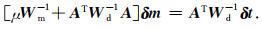
|
(2) |
方程(2)可采用共轭梯度法(Zhou et al., 1992)迭代求解,但是每次迭代都需要重新进行射线追踪并计算Frechet偏导数矩阵A.
2.2 Frechet偏导数计算微地震定位和各向异性速度结构同时反演时,Frechet偏导数矩阵包含三部分:一是到时关于Thomsen参数的导数,二是到时关于界面深度的导数,三是到时关于微震源参数的导数,即:
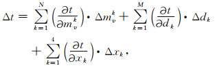
|
(3) |
其中mvk和dk分别是第k层的Thomsen参数和与射线相交的第k个层界面的深度,Δmvk和Δdk则是相应的扰动量.N是模型层数,M是射线穿过的界面层数.Δxk(k=1, 2, 3, 4)分别是第k个微震事件的空间坐标(x、y、z)和发震时刻的扰动量.
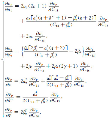
2.2.1 到时关于Thomsen参数的一阶偏导数到时关于Thomsen参数的一阶偏导数可以从走时的一阶扰动方程(Zhou and Greenhalgh, 2008)获得:
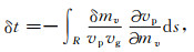
|
(4) |
式中vp和vg分别代表相速度和群速度,R是射线路径,ds代表模型参数化后单元格内的射线长度.根据方程(4),到时关于第k层Thomsen参数的一阶偏导数可写为:
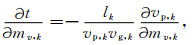
|
(5) |
式中lk是射线在第k层内的长度,vp, k和vg, k分别是第k层的相速度和群速度.相速度关于Thomsen参数的导数采用下列公式计算(Zhou and Greenhalgh, 2008):
|
(6) |
到时关于发震时刻的一阶偏导数可以直接从到时公式t=t0+T得到:

|
(7) |
其中t0是发震时刻,T是走时.
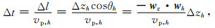
而到时关于微地震事件空间坐标的一阶偏导数的计算公式可参见图 2.假设震源深度扰动Δzh,则到时的变化为:

|
图 2 震源深度Δzh变化引起到时的扰动 Fig. 2 The change in depth Δzh of the hypocenter results in a perturbation on the arrival time |
|
(8) |
式中θh是相慢度矢量wh与Z轴的夹角,vp, h是震源处相慢度方向的相速度值,单位向量wz=(0, 0, 1)和wh如图 2所示.因此,到时关于震源深度的一阶偏导数为

|
(9) |
同理可得到时关于震源位置其余两个方向(x、y)的偏导数为:

|
(10) |
其中单位向量wx=(1, 0, 0),wy=(0, 1, 0).
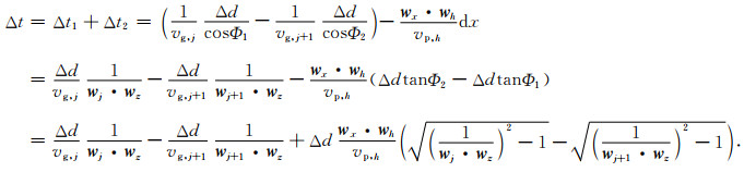
2.2.3 到时关于界面深度的一阶偏导数图 3显示了由界面深度扰动引起的射线路径和到时的变化.遵循Snell定律,界面深度发生变化后,接收器R处的地震波可认为来自虚拟源Sv.接收器R的到时扰动可以分解为两部分:(1)由群速度和射线路径变化引起的到时变化Δt1;(2)震源位置从S变化到Sv引起的到时变化Δt2.因此,由界面深度变化引起的到时扰动可表示为

|
图 3 由界面深度变化引起的射线路径和到时扰动 S表示震源,R表示接收器.介质1和介质2的群角和群速度分别表示为Φ1、vg, j和Φ2、vg, j+1.扰动前的射线路径和界面用实线表示,扰动后的用虚线表示.wj和wj+1分别是与入射射线和出射射线平行的单位向量. Fig. 3 Ray paths and traveltime perturbations caused by the layer interface variations S denotes the source and R denotes the receiver. The group angle and group velocity are Φ1, vg, j in the first medium, and Φ2, vg, j+1 in the second medium, respectively. The original ray path and interface are denoted by the solid line and the perturbed ray path and interface are denoted by the dashed lines. wj is a unit vector parallel to incident rays and wj+1 is a unit vector parallel to ejected rays. |
|
(11) |
则到时关于界面深度的一阶偏导数为

|
(12) |
式中vg, j和vg, j+1分别是界面上、下的群速度,单位向量wj, wj+1, wz如图 3所示.值得注意的是,公式(12)对于任意射线方向都是有效的,无论射线是向上传播,还是向下传播.但必须保证wj始终指向界面,wj+1始终背离界面.而且,公式(12)也适用于多层情况.在确定射线与层界面的所有交点之后,可以将这些交点替换为图 3所示震源和接收器位置来计算到时关于每层界面深度的偏导数.
3 数值模拟分析为了验证该算法的有效性及实用性,本文选择一个3-D TI模型来同时反演各向异性速度结构(Thomsen参数和界面深度)和微震震源参数(空间坐标和发震时刻).Zhou和Greenhalgh(2008)指出如果同时反演对称轴角度(θ0,φ0),反演效果不理想.这是因为相速度和到时关于对称轴角度(θ0,φ0)高度敏感.因此,这里我们假设介质的对称轴角度已知,仅各节点上的5个Thomsen参数未知.qP、qSV和qSH波的到时采用第1节中介绍的改进最短路径算法计算.根据反演理论,方程(2)中的加权矩阵(Wd-1和Wm-1)可根据数据噪声和模型参数变化的先验信息(Menke, 1984;Tarantola, 1987;Carrion, 1989)确定,以降低解的非唯一性.本文假设加权矩阵为单位矩阵,这意味着没有先验信息可用.假设三种波的拾取精度相同(p1=p2=…=pn=1),通过实验计算,根据到时残差的收敛情况选择最佳阻尼因子μ.
3-D模型如图 1所示,尺寸为300 m×300 m×300 m,网格尺寸为10 m×10 m×10 m.层界面深度分别为80 m、130 m和200 m,各层Thomsen参数如表 1所示.为模拟地面和井中微地震,采用实际微地震中常用的地表“米”字和井中联合观测方式(图 1中三角形),地表 24个检波器,井中14个地震检波器.两个裂缝系统如图 1所示.每个裂缝系统由两个相邻的平行裂缝组成,每个裂缝有四个微地震事件,四个事件的发震时刻分别为5 ms、10 ms、15 ms和20 ms.
|
|
表 1 模型各层Thomsen参数 Table 1 Thomsen parameters of each layer in the model |
反演采用三种波(初至qP、qSV和qSH波)的到时.图 4给出了图 1裂缝系统中两个事件的qP波射线路径.从图中可以看出,不同层的射线角度覆盖范围不同,第三层为低速层,因此地震波在第二界面和第三界面处发生滑行现象.

|
图 4 裂缝系统中两个事件的qP波射线路径.不同微震事件的射线路径以灰色和黑色区分 Fig. 4 The ray paths of the qP waves for the two events corresponding to the fractures. And the ray paths of different microseismic events are distinguished by gray and black |
首先在理想条件下(正确的各向异性速度模型、无噪声)讨论该反演算法进行微地震定位的能力.16个事件的初始震源位置均为(150, 150, 150)m,初始发震时刻均为0 ms.裂缝系统的定位结果如图 5所示,即使初始震源参数离真实值较远,反演的震源空间坐标位置(图 5a—5c)和发震时刻(图 5d)都与理论参数完全一致.

|
图 5 理想条件下的微地震定位结果 (a) x-y平面;(b) x-z平面;(c) y-z平面;(d) x-t0平面.其中灰色代表真实值,浅灰色十字代表初始值,黑色代表反演值. Fig. 5 Microseismic location results under the ideal conditions (a) x-y plane; (b) x-z plane; (c) y-z plane; (d) x-t0 plane. Gray symbols indicate the real values, and light gray crosses indicate the initial values. The black symbols indicate the inverted values. |
然而实际数据处理中不可能满足理想条件,例如地下介质的各向异性速度结构(各层Thomsen参数和界面深度)未知、数据包含噪声、各向异性及非均匀性等.因此,本文下面给出该反演算法同时进行各向异性速度结构模型反演和微地震定位的结果,并讨论其对噪声及各向异性非均匀性的敏感性.同时反演的初始模型参数设置如下:将第一层的Thomsen参数值作为各层的反演初始值;各层的界面深度的初始值与真实值存在10 m的差异;各震源的初始位置和发震时刻均相同,分别为(150, 150, 150)m和0 ms.
图 6和图 7是无噪声时同时反演的结果.从微震定位结果(图 6)可以看出,微震事件以相对位置的方式恢复,例如,裂缝被成功描绘,显示出清晰的平行结构,但与正确的结构位置存在差异.图 7中的5个Thomsen参数的反演恢复程度是不同的.例如,第二层的α0反演结果较差,与真实值差异较大(参见图 7a).这是因为,尽管射线覆盖相同,但到时对于参数的敏感性并不相同(公式(6)).即使对于相同的Thomsen参数,其敏感性也随射线角度变化,因此各层的Thomsen参数的恢复程度也各不相同.例如第二层的5个Thomsen参数反演效果相对较差.且Thomsen参数和界面深度在反演时两者之间存在关联性,当第一层界面的深度反演结果较差时(图 7b),就出现了第二层的Thomsen参数的反演效果不好的情况(图 7a).因此,当射线的角度覆盖较好时,同时进行各向异性速度结构反演和微地震定位是可行的,反演精度较高.

|
图 6 微地震定位结果 图(a)—(c)分别是x-y、x-z和y-z面的微地震定位结果,图(d)是震源发震时刻的反演结果.其中灰色代表真实值,浅灰色十字代表初始值,黑色代表反演值. Fig. 6 Microseismic location results Panels (a)—(c) show the relocated spatial coordinates in the x-y, x-z and y-z planes, respectively, and panel (d) is the inverted origin time. Gray symbols indicate the real values, and light gray crosses indicate the initial values. The black symbols indicate the inverted values. |

|
图 7 Thomsen参数和层界面深度的反演值与真实值的对比 灰色和黑色分别代表真实参数值和更新值.Thomsen参数中的上标代表层编号.括号内数值代表绝对误差值. Fig. 7 Comparison between the true values of Thomsen parameters and layer interface depth and the inverted Gray and black symbols stand for the true parameter values and the updated values, respectively. The superscript in the Thomsen parameters denotes the layer numbers. The values in parentheses represent absolute errors. |
考虑拾取初至时可能存在误差,在理论的初至qP、qSV和qSH波到时数据中加入5%的随机噪声.含噪声到时数据同时反演的结果如图 8(微震定位结果)和表 2(各向异性速度结构反演误差)所示.对比分析图 8和表 2含噪声同时反演结果和无噪声同时反演结果,结果显示:当到时中包含噪声时,同时反演精度均有所下降.加入随机噪声后,对微地震定位精度影响不大,且对微地震震源水平位置的定位(图 8a)明显好于震源深度的定位(图 8b和图 8c).各向异性速度结构层析的结果变化较大(表 2),Thomsen参数和界面深度都存在一定程度的偏差.这是由于当各向异性速度结构层析和微地震定位同时进行时,两者的反演结果实际上是一定程度的折中.总体而言,微地震定位对到时中的随机噪声不敏感.

|
图 8 到时数据中加入5%的随机噪声时的微地震定位结果 其中红色代表真实值,蓝色十字代表初始值,绿色代表无噪声时反演值,紫色代表数据含噪声时的反演值. Fig. 8 Microseismic location results with 5% random noise Red symbols indicate the real values, and blue crosses indicate the initial values. The green symbols indicate the inverted values without random noise. The purple symbols indicate the inverted values with random noise. |
|
|
表 2 有随机噪声和无随机噪声时反演的Thomsen参数和层界面深度值的误差 Table 2 Errors in inverted Thomsen parameters and layer interface depth values with or without random noise |
进一步采用图 9中所示的各向异性模型来测试该方法对各向异性非均匀性的敏感性.该各向异性非均匀模型是对前面模拟中的层状TI介质模型进行随机扰动得到的.5个Thomsen参数分别加入随机扰动,随机扰动的最大幅值为15%:

|
图 9 α0随机扰动模型 Fig. 9 Randomly-perturbed model for α0 |

|
(13) |
其中R表示随机数.观察到时是采用图 9所示的非均匀各向异性模型计算得到的,但同时反演时所采用的模型为均匀的1-D层状TI模型.反演参数的初始值与无噪声同时反演时相同.图 10为微震定位结果.反演的事件位置与真实的事件位置略有不同,特别是震源深度(图 10),但事件的相对位置恢复的相对较好,仍能刻画出裂缝的平行结构.图 11给出了各向异性速度结构层析结果.各层的Thomsen参数和界面深度的反演精度各不相同,都与近似的均匀1-D的TI模型存在一定程度的差异.

|
图 10 使用随机扰动模型时微地震定位结果 其中灰色代表真实值,浅灰色十字代表初始值,黑色代表反演值. Fig. 10 Microseismic location results by using the randomly-perturbed velocity model Gray symbols indicate the real values, and light gray crosses indicate the initial values. The black symbols indicate the inverted values. |

|
图 11 随机扰动模型Thomsen参数和层界面深度的反演值与真实值间的对比 灰色圆点和黑色三角分别代表真实值和反演值.括号内数值代表绝对误差值. Fig. 11 Comparisons between the true values of Thomsen parameters and layer interface depths with the inverted results in the randomly-perturbed model Gray dots and black triangles indicate the true and inverted values, respectively. The values in parentheses represent absolute errors. |
为降低速度模型估计不准确对微震定位精度的影响,本文提出了一种在1-D层状TI介质中同时反演各向异性速度结构模型和微地震定位的算法.首先采用基于界面元的改进最短路径算法计算初至波的射线路径和到时,然后导出到时关于Thomsen参数、层界面深度、震源空间坐标和发震时刻的偏导数,再结合共轭梯度法求解带约束的阻尼最小二乘问题,发展了一种同时反演各向异性速度结构模型(Thomsen参数和界面深度)和震源参数(空间坐标和发震时刻)的方法.地面和井中联合观测条件下的数值模拟结果表明:当射线角度覆盖良好时,该算法能有效地反演地下的各向异性速度结构并进行微地震定位,并且微地震定位结果对到时中的随机噪声和包含在模型中的各向异性非均匀性不是特别敏感.
本文采用理论合成数据验证了所提方法的有效性,虽然考虑了数据含噪声及各向异性模型的非均匀性,但在实际生产中,还存在其他诸如地层起伏不平、数据信噪比低的因素,因此在未来研究中,有必要结合实际数据与现场地质情况,应用、测试本文方法的可靠性及稳健性,从而进一步提高实际定位精度.
Agostinetti N P, Giacomuzzi G, Malinverno A. 2015. Local three-dimensional earthquake tomography by trans-dimensional Monte Carlo sampling. Geophysical Journal International, 201(3): 1598-1617. DOI:10.1093/gji/ggv084 |
Aki K, Lee W H K. 1976. Determination of three-dimensional velocity anomalies under a seismic array using first P arrival times from local earthquakes:1. A homogeneous initial model. Journal of Geophysical Research, 81(23): 4381-4399. DOI:10.1029/JB081i023p04381 |
Albright J N, Pearson C F. 1982. Acoustic emissions as a tool forhydraulic fracture location:experience at the Fenton Hill hot dry rock site. Society of Petroleum Engineers Journal, 22(4): 523-530. DOI:10.2118/9509-PA |
Bai C Y, Tang X P, Zhao R. 2009. 2-D/3-D multiply transmitted, converted and reflected arrivals in complex layered media with the modified shortest path method. Geophysical Journal International, 179(1): 201-214. DOI:10.1111/j.1365-246X.2009.04213.x |
Bai C Y, Huang G J, Zhao R. 2010. 2-D/3-D irregular shortest-path ray tracing for multiple arrivals and its applications. Geophysical Journal International, 183(3): 1596-1612. DOI:10.1111/j.1365-246X.2010.04817.x |
Block L V, Cheng C H, Fehler M C, et al. 1994. Seismic imaging using microearthquakes induced by hydraulic fracturing. Geophysics, 59(1): 102-112. |
Carcione J M. 2014. Wave fields in real media.//Theory and Numerical Simulation of Wave Propagation in Anisotropic, Anelastic, Porous and Electromagnetic Media. 3rd ed. Amsterdam: Elsevier.
|
Carrion P M. 1989. Generalized non-linear elastic inversion with constraints in model and data spaces. Geophysical Journal International, 96(1): 151-162. DOI:10.1111/j.1365-246X.1989.tb05257.x |
Eberhart-Phillips D. 1990. Three-dimensional P and S velocity structure in the Coalinga Region, California. Journal of Geophysical Research:Solid Earth, 95(B10): 15343-15363. DOI:10.1029/JB095iB10p15343 |
Grechka V. 2010. Data-acquisition design for microseismic monitoring. The Leading Edge, 29(3): 278-282. DOI:10.1190/1.3353723 |
Grechka V, Singh P, Das I. 2011. Estimation of effective anisotropy simultaneously with locations of microseismic events. Geophysics, 76(6): WC143-WC155. DOI:10.1190/geo2010-0409.1 |
Grechka V, Yaskevich S. 2013. Inversion of microseismic data for triclinic velocity models. Geophysical Prospecting, 61(6): 1159-1170. DOI:10.1111/1365-2478.12042 |
He L Y, Bai C Y, Wang D. 2019. Anisotropic crosshole+VSP traveltime tomography through triangular cell model with a normalized Jacobian matrix and multistage inversion strategy. Pure and Applied Geophysics, 176(1): 235-255. |
Huang G J, Bai C Y, Qian W. 2015. Simultaneous inversion of three model parameters with multiple phases of arrival times in spherical coordinates. Chinese Journal of Geophysics (in Chinese), 58(10): 3627-3638. DOI:10.6038/cjg20151016 |
Husen S, Quintero R, Kissling E, et al. 2003. Subduction-zone structure and magmatic processes beneath Costa Rica constrained by local earthquake tomography and petrological modelling. Geophysical Journal International, 155(1): 11-32. DOI:10.1046/j.1365-246X.2003.01984.x |
Iyer H M, Hirahara K. 1993. Seismic tomography:Theory and practice. London: Springer.
|
Li J L, Zhang H J, Rodi W L, et al. 2013. Joint microseismic location and anisotropic tomography using differential arrival times and differential backazimuths. Geophysical Journal International, 195(3): 1917-1931. DOI:10.1093/gji/ggt358 |
Li J L, Li C, Morton S A, et al. 2014. Microseismic joint location and anisotropic velocity inversion for hydraulic fracturing in a tight Bakken reservoir. Geophysics, 79(5): C111-C122. DOI:10.1190/geo2013-0345.1 |
Martakis N, Kapotas S, Tselentis G A. 2006. Integrated passive seismic acquisition and methodology:Case studies. Geophysical Prospecting, 54(6): 829-847. DOI:10.1111/j.1365-2478.2006.00584.x |
Maxwell S C, Rutledge J, Jones R, et al. 2010a. Petroleum reservoir characterization using downhole microseismic monitoring. Geophysics, 75(5): 75A. |
Maxwell S C, Bennett L, Jones M, et al. 2010b. Anisotropic velocity modeling for microseismic processing: Part 1-Impact of velocity model uncertainty.//80th Ann. Internat Mtg., Soc. Expi. Geophys.. Expanded Abstracts, 2130-2134.
|
Menke W. 1984. Geophysical Data Analysis:Discrete Inverse Theory. New York: Academic Press Inc.: 40-126.
|
Ochoa-Chávez J A, Escudero C R, Núñez-Cornú F J, et al. 2016. P-wave velocity tomography from local earthquakes in Western Mexico. Pure and Applied Geophysics, 173(10): 3487-3511. |
Paul A, Cattaneo M, Thouvenot F, et al. 2001. A three-dimensional crustal velocity model of the southwestern Alps from local earthquake tomography. Journal of Geophysical Research:Solid Earth, 106(B9): 19367-19389. DOI:10.1029/2001JB000388 |
Pei D H, Quirein J A, Cornish B E, et al. 2009. Velocity calibration for microseismic monitoring:A very fast simulated annealing (VFSA) approach for joint-objective optimization. Geophysics, 74(6): WCB47-WCB55. DOI:10.1190/1.3238365 |
Rawlinson N, Sambridge M. 2004. Multiple reflection and transmission phases in complex layered media using a multistage fast marching method. Geophysics, 69(5): 1338-1350. DOI:10.1190/1.1801950 |
Rutledge J T, Phillips W S. 2003. Hydraulic stimulation of natural fractures as revealed by induced microearthquakes, Carthage Cotton Valley gas field, east Texas. Geophysics, 68(2): 441-452. |
Rutledge J T, Phillips W S, Mayerhofer M J. 2004. Faulting induced by forced fluid injection and fluid flow forced by faulting:an interpretation of hydraulic-fracture Microseismicity, Carthage cotton valley gas field, Texas. Bulletin of the Seismological Society of America, 94(5): 1817-1830. DOI:10.1785/012003257 |
Tarantola A. 1987. Inverse Problem Theory, Methods for Data Fitting and Model Parameter Estimation. Amsterdam: Elsevier.
|
Thomsen L. 1986. Weak elastic anisotropy. Geophysics, 51(10): 1954-1966. DOI:10.1190/1.1442051 |
Thurber C H. 1983. Earthquake locations and three-dimensional crustal structure in the Coyote Lake area, central California. Journal of Geophysical Research:Solid Earth, 88(B10): 8226-8236. DOI:10.1029/JB088iB10p08226 |
Tsvankin I, Grechka V. 2011. Seismology of azimuthally anisotropic media and seismic fracture characterization.//81st Ann. Internat Mtg., Soc. Expi. Geophys.. Expanded Abstracts.
|
Wang H, Li M, Shang X F. 2016. Current developments on micro-seismic data processing. Journal of Natural Gas Science and Engineering, 32: 521-537. DOI:10.1016/j.jngse.2016.02.058 |
Warpinski N R, Sullivan R B, Uhl J E, et al. 2005. Improved microseismic fracture mapping using perforation timing measurements for velocity calibration.//73rd Ann. Internat Mtg., Soc. Expi. Geophys.. Expanded Abstracts, 84488.
|
Yolsal-ßevikbilen S, Biryol C B, Beck S, et al. 2012. 3-D crustal structure along the North Anatolian Fault Zone in north-central Anatolia revealed by local earthquake tomography. Geophysical Journal International, 188(3): 819-849. DOI:10.1111/j.1365-246X.2011.05313.x |
Yuan D, Li A B. 2017. Joint inversion for effective anisotropic velocity model and event locations using S-wave splitting measurements from downhole microseismic data. Geophysics, 82(3): C133-C143. DOI:10.1190/geo2016-0221.1 |
Zhang G M. 2010. A numerical simulation study on hydraulic fracturing of horizontal well[Ph. D. thesis] (in Chinese). Hefei: University of Science and Technology of China.
|
Zhang H H, Sarkar S, Toksöz M N, et al. 2009. Passive seismic tomography using induced seismicity at a petroleum field in Oman. Geophysics, 74(6): WCB57-WCB69. DOI:10.1190/1.3253059 |
Zhang H J, Thurber C H. 2003. Double-difference tomography:The method and its application to the Hayward fault, California. Bulletin of the Seismological Society of America, 93(5): 1875-1889. DOI:10.1785/0120020190 |
Zhang S, Liu Q L, Zhao Q, et al. 2002. Application of microseismic monitoring technology in development of oil field. Geophysical Prospecting for Petroleum (in Chinese), 41(2): 226-231. |
Zhang X L, Zhang F, Li X Y, et al. 2013. The influence of hydraulic fracturing on velocity and microseismic location. Chinese Journal of Geophysics (in Chinese), 56(10): 3552-3560. DOI:10.6038/cjg20131030 |
Zhao D P, Hasegawa A, Horiuchi S. 1992. Tomographic imaging of P and S wave velocity structure beneath Northeastern Japan. Journal of Geophysical Research:Solid Earth, 97(B13): 19909-19928. DOI:10.1029/92JB00603 |
Zhao R, Bai C Y. 2010. Fast multiple ray tracing within complex layered media:The shortest path method based on irregular grid cells. Acta Seismologica Sinica (in Chinese), 32(4): 433-444. |
Zheng Y K, Wang Y B, Chang X. 2016. Wave equation based microseismic source location and velocity inversion. Physics of the Earth and Planetary Interiors, 261: 46-53. DOI:10.1016/j.pepi.2016.07.003 |
Zhou B, Greenhalgh S A, Sinadinovski C. 1992. Iterative algorithm for the damped minimum norm, least-squares and constrained problem in seismic tomography. Exploration Geophysics, 23(3): 497-505. DOI:10.1071/EG992497 |
Zhou B, Greenhalgh S A. 2004. On the computation of elastic wave group velocities for a general anisotropic medium. Journal of Geophysics and Engineering, 1(3): 205-215. |
Zhou B, Greenhalgh S A. 2008. Non-linear traveltime inversion for 3-D seismic tomography in strongly anisotropic media. Geophysical Journal International, 172(1): 383-394. DOI:10.1111/j.1365-246X.2007.03649.x |
黄国娇, 白超英, 钱卫. 2015. 球坐标系下多震相走时三参数同时反演成像. 地球物理学报, 58(10): 3552-3560. DOI:10.6038/cjg20151016 |
张广明. 2010.水平井水力压裂数值模拟研究[博士论文].合肥: 中国科学技术大学.
|
张山, 刘清林, 赵群, 等. 2002. 微地震监测技术在油田开发中的应用. 石油物探, 41(2): 226-231. DOI:10.3969/j.issn.1000-1441.2002.02.021 |
张晓林, 张峰, 李向阳, 等. 2013. 水力压裂对速度场及微地震定位的影响. 地球物理学报, 58(10): 3552-3560. DOI:10.6038/cjg20131030 |
赵瑞, 白超英. 2010. 复杂层状模型中多次波快速追踪:一种基于非规则网格的最短路径算法. 地震学报, 32(4): 433-444. DOI:10.3969/j.issn.0253-3782.2010.04.006 |