 2020, Vol. 63


2. Laboratoire de Geophysique Interne et de Tectonophysique, Université Joseph Fourier, CNRS, Grenoble 38000, France
2. Laboratoire de Geophysique Interne et de Tectonophysique, Université Joseph Fourier, CNRS, Grenoble 38000, France
地震环境噪声技术(ANT)是近十几年来地震学领域迅速发展起来的一个重要方法,地壳及地幔顶部的面波层析成像是其重要应用之一.不同于依赖地震事件发生的传统面波成像方法,ANT基于随机波场的互相关方法提取面波格林函数(Campillo and Paul, 2003; Shapiro and Campillo, 2004; Sabra et al., 2005a; Pedersen and Krüger, 2007;齐诚等,2007),该方法可以克服传统面波成像中的很多问题,尤其是诸如缺乏广泛分布的地震源、远震高频频散提取困难等问题,因而,地震环境噪声成像方法已经在世界各地取得了广泛的应用(Shapiro et al., 2005; Sabra et al., 2005b; Yao et al., 2006, 2008; Stehly et al., 2009; Ritzwoller et al., 2011; Li et al., 2013; 房立华等,2009;李昱等,2010;庞广华等,2014;赵盼盼等,2015).
地震环境噪声成像方法一般包含几个步骤:地震环境噪声数据预处理、噪声互相关函数计算、面波频散曲线提取、面波层析成像、S波速度结构反演.需要注意的是,常规的环境噪声成像方法一般采用与传统地震面波频散反演方法相同的S波速度结构反演方法(Hermann and Ammon, 2002),对于长周期、数十千米分辨率尺度的地壳和上地幔速度结构研究,基于一维平层假定,几百米甚至2~3 km的地形高程起伏差异通常不需要考虑.
近年来,流动地震台阵观测技术逐渐从传统的针对大尺度地壳和岩石圈结构研究(Moschetti et al., 2009; Chu et al., 2013; 陈兆辉等,2014;Huang et al., 2015; Xu et al., 2018; Guo et al., 2019; 郭慧丽等,2017;钟世军等,2017;郑晨等,2018)向小尺度密集台阵探测研究发展(Lin et al., 2013; Liu et al., 2017b), 逐渐开展千米级分辨率的地下结构探测研究.Wang和Sun(2019)探讨了地形起伏对短周期环境噪声成像结果的影响,认为地表地形起伏超过一定程度会对探测结果具有不可忽视的影响.在我国的一些重要地区,例如青藏高原东缘的龙门山地区,几十千米距离内地形起伏就达到了几千米的差异,在这样的特殊地区开展高分辨率速度结构探测,解决地形对成像结果的影响是十分必要的工作.
传统的一维和二维反演是对介质结构进行适当简化后进行的,当地下介质存在非均匀结构时,描述介质内传播的波场需要以三维介质结构为基础.当地表存在无法忽略的地形因素时,要描述介质的波场特征则是典型的三维问题.面波频散反演则需要通过波形反演来进行.地震学家早在20世纪80年代就开始尝试反演地震波形来获得结构信息(Woodhouse and Dziewonski, 1984),然而由于波形反演技术大大增加了计算的复杂度和非线性程度,且对计算能力和内存要求高,在实际数据解释的应用中难度很高.虽然随着计算能力的增强,以及在Tarantola(1984)发展的全波形反演理论中引入伴随方法,三维环境噪声层析成像也取得了较大的发展(Tromp et al., 2005; Tape et al., 2007; 2009;Liu and Gu, 2012; Zhu et al., 2012),但是在实际工作中采用三维波形反演研究地壳上地幔速度结构仍然是件复杂且计算量巨大的工作(Chen et al., 2014, 2015; Liu et al., 2017a).
本文针对研究区域存在巨大地表地形差异情况,尝试通过地震波场三维正演模拟和频散曲线校正,建立适合消除地表地形巨大差异对使用地震环境噪声面波成像方法研究地壳速度结构影响的方法,以达到在计算量和难度都较小的情况下对研究区进行了准三维结构反演的目的.
1 地形影响校正方法传统的地震环境噪声面波成像方法一般在提取台站间面波频散曲线的基础上,首先反演获得不同周期的面波群速度分布(Barmin et al., 2001),随后根据各格点的面波频散曲线反演得到随深度变化的S波速度模型(Hermann and Ammon, 2002).这一两步反演法可以简单有效的构建出速度模型.其中,线性反演迭代是使某观测参数(这里是群速度)与模型预测参数之间误差达到最优化.我们在这里保留简单的两步法不变,考虑如何获得更加接近真实的模型.显然,该模型必须考虑到研究区域地形起伏导致的诸如瑞利波延时、散射等问题.
我们采用的方案是首先用上述传统环境噪声成像方法获得一个初始的参考S波速度模型,忽略地形、散射等因素的影响.以此一维速度结构为基础,我们构建一个包含地形的三维地壳速度模型.地表高程部分的速度是未知的,考虑到速度结构的可靠性和连续性,我们将地表高程部分的速度取垂直对应的各三维模型格点处一维速度模型的表层S波速度.在与研究中使用的真实台站分布相一致的位置分别以垂直点源作为震源,以其他台站作为接收点,计算出各台站间的理论地震波.随后,与处理实际观测的地震环境噪声数据的方法类似,我们提取台站间的瑞利波群速度频散曲线,并反演每个格点的群速度,记为Usimu(i, T).其中,i表示不同格点,T表示不同周期.此外,我们将由真实观测地震环境噪声数据的面波反演所得各格点瑞利波群速度记为Uobs(i, T),由Uobs(i, T)可以反演得到忽略地形高程影响的一维参考S波速度模型,以及与之对应的瑞利波群速度频散曲线,记为U0(i, T).于是,我们可以将地形高程带来的影响近似定义为

|
(1) |
对于由观测数据所得瑞利波群速度Uobs(i, T)进行校正以去除地形高程影响:

|
(2) |
最后,以校正后的群速度U′obs(i, T)反演得到新的S波速度结构(图 1).

|
图 1 地形校正方法流程图 Fig. 1 Flowchart of topography correction in seismic topography |
龙门山断裂带位于四川盆地与松潘—甘孜块体交界,该区域的高程从四川盆地的几百米变化到松潘高原的4~5 km.特别在两个块体的边界地区,存在非常大的跳跃式地形变化.因此,我们以龙门山断裂带及周边区域这一极具代表性的地区为例研究地表地形高程对地壳速度结构的地震环境噪声成像结果影响.
为了获得理论观测数据,本文使用了Etienne等(2010)提出的一种适合大规模地震波模拟的结合卷积完全匹配层(CMPL)吸收边界条件(Roden and Gedney, 2000; Komatitsch and Martin, 2007)的hp自适应低阶不连续伽辽金有限元方法(DG-FEM)进行地震波场三维正演模拟.该方法使用非结构化的四面体网格划分,并根据介质特性进行局部完善(h自适应);与此同时,不同单元的逼近阶次根据一个适当的标准而变化(p自适应).其中,p自适应对于DG-FEM尤为重要.在模拟时,一般会遇到由于局部完善而出现的很小的单元,p自适应为减轻这些微小单元的影响从而进行高效模拟提供了保障,它根据单元的大小以及介质的特性调节逼近阶次,以获得最优化的时步.对于强烈非均匀介质,这一点更加重要.
我们分别通过在三个三维速度模型中模拟地震波传播,而后进行地形校正处理前后的S波速度反演结果对比,以检验地形校正方法的有效性.考虑到在后文中我们将把该方法应用于龙门山地区实际观测数据的处理中,在此,我们构建的三维理论速度结构模型的水平范围覆盖了所用的全部地震观测台站,如图 2a所示.我们将模型简化为三个块体,并在各块体分别给定一个随深度变化的S波速度结构,如图 2b所示.地表高程起伏对于研究浅层精细速度结构影响较大,因此我们增强了模型浅层速度结构的差异性,而较深部分速度结构差异较小,并且三个块体速度高低在浅部与深部不同,使得该模型具有较强的对比度,同时也具有一定的复杂性与一般代表性.模型的垂直范围包含地表高程至水平面以下40 km深度.检验过程主要是针对不同地表高程带来的影响及校正情况,三个模型的差异也在于此,分别为零高程、三块式高程分布以及对应龙门山区域真实的地表高程,如图 2c、d、e所示.模型的网格大小为1 km×1 km.模型构建过程中需要在模型除地表外的四周及底部额外添加边界吸收层,如图 3所示.Etienne等(2010)对于该三维模拟方法中吸收层的设置及其影响有详细的测试,其结果表明,20个单元宽度的吸收层即可以满足需求,而每个单元宽度大约为三分之一最小波长.本文模拟中使用的Ricker子波震源主频率为0.2 Hz,最大频率约为0.5 Hz,假设面波速度为3 km·s-1,最小波长即为6 km,那么吸收层的宽度为40 km.吸收层的速度结构为未添加该层前的三维模型相应表层速度的外部扩展.

|
图 2 (a) 以虚线划分的模型水平区域分块图,三个块体分别代表四川盆地(SC)、龙门山断裂带(LMS)、松潘高原(SP),灰色细线表示断层,黑色三角表示地震台站;(b)不同区域给定的S波速度结构模型;(c)零高程模型垂直剖面速度结构示意图,剖面位置如图 2a黑色直线所示;(d)三块式高程模型垂直剖面速度结构示意图;(e)真实高程模型垂直剖面速度结构示意图 Fig. 2 (a) Horizontal zoning map of the model divided by dotted lines. Three blocks represent Sichuan basin (SC), Longmenshan fault zone (LMS) and Songpan plateau (SP), respectively. Gray lines are faults. Black triangles are seismic stations; (b) Structural model of S wave velocity for different regions; (c) The velocity structure of the vertical section presented by solid black line in Fig. 2a of the zero-elevation model; (d) The velocity structure of the vertical section of the model with elevation variation for three blocks; (e) The velocity structure of the vertical section of the model with the true surface of the Longmenshan area |

|
图 3 对应于图 2e的三维模型地表示意图(图 3b在图 3a基础上添加了吸收层) Fig. 3 Surface map of the 3D model corresponding to Fig. 2e(An absorbed layer is added in Fig. 3b) |
基于给定的初始速度结构(图 2b)建立三维模型后,分别以与真实观测台站位置相同的台站之一作为垂直点源位置,以其他台站作为接收点,就可以得到各台站间的模拟地震波数据.图 4以真实高程模型(图 2e)为例,给出了两个不同震源的地震波场数值模拟图.图 5a绿色曲线所示为台站间的合成地震记录, 我们将其视为原始观测数据.对于零高程模型、三块式高程模型与真实高程模型,获得原始观测数据方法相同.利用前文所述传统的面波成像方法,可以得到如图 6b、图 7b、图 8b所示的分别对应于零高程模型、三块式高程模型与真实高程模型的不同深度S波速度分布.同时,三个模型对应深度的真实S波速度分布相同且如图 6a、图 7a、图 8a所示.对于零高程模型,图 6a、b在速度值大小上存在差异但不十分显著,同时区域分布特征清晰可见,说明通过三维模拟所得地震数据再次反演的结果虽然不能完全复原模型的速度结构,但也可以基本反映出模型的真实结构.对于三块式高程模型与真实高程模型,由图 7b、图 8b可见S波速度反演结果与真实速度分布都有较大差异.反演结果可以看出一定的区域分布特征但不够清晰.同时,速度值大小与真实情况有显著差异,速度值反演结果偏低.这两组对比反映出地形高程对噪声成像工作存在的不良影响.随后,我们对于这两种模型反演结果分别进行如第1节所述的地形校正,得到了如图 7c、图 8c所示的S波速度分布.虽然地形校正后的反演结果与真实速度模型仍然存在一定差异,最终获得的速度图像仍然存在着地表高程和散射效应等带来的干扰,但经过校正后的反演图像明显更接近真实速度模型,修正后的结果真实反映了真实模型的速度结构特征.并且,对于两种不同的地形高程情况,修正后都得到了较好的结果.这些试验显示了在地形高程影响较大的区域开展噪声成像工作时进行地形校正的必要性以及该校正方法的有效性.

|
图 4 真实高程模型中地震波场数值模拟(震源位置分别如图 3红色三角所示) Fig. 4 3D seismic wavefield numerical simulation in the model with true surface of the Longmenshan area (The black triangle indicates the source location shown in Fig. 3) |

|
图 5 (a) 绿色曲线代表在真实高程模型测试过程中的初始速度结构模型下,分别位于LX12、MA02、MZ14和MG22台站位置的接收点记录到的HS13台站位置的震源发出的地震波波形,各台站位置见图 3;红色与蓝色曲线分别代表在以未做与已做地形校正的速度结构反演结果构建的模型下记录的相同震源与接收点的地震波波形;(b)分别对应图 5a中HS13震源与MZ14接收点间(HS13-MZ14)三个地震波形的瑞利波群速度频散曲线;(c)不同周期瑞利波群速度均方根差.红色与蓝色方形分别对应未做与已做地形校正 Fig. 5 (a) The green curves represent the seismic waveforms from the source located atthe station HS13 recorded at the station LX12, MA02, MZ14 and MG22, respectively, under the initial velocity structure in the test process of the real elevation model.The station position is shown in Fig. 3.The blue and red curves represent the seismic waveforms from the same source to the receiver recorded under the model constructed by inversion results with and without topographic correction; (b) The Rayleigh-wave group-velocity dispersion curves of three seismic waveforms between source HS13 and receiver MZ14(HS13-MZ14)corresponding to the three seismic waveforms in Fig. 5a; (c) The RMSE of the Rayleigh-wave group-velocity for different periods. The blue and red squares correspond to the corrected and uncorrected models |

|
图 6 零高程模型三维模拟的反演测试 (a)不同深度S波速度真实模型;(b)不同深度S波速度反演结果. Fig. 6 Inversion test for 3D simulation of zero-elevation model (a) The S-wave velocity model at different depths; (b) Inversion results of S-wave velocity at different depths. |

|
图 7 三块式高程模型中地形校正方法测试 (a)不同深度S波速度真实模型;(b)未做地形校正的反演结果;(c)地形校正后的反演结果. Fig. 7 Test of the topography correction method in the model with elevation variation for three blocks (a) The S-wave velocity model at different depths; (b) The surface wave imaging without the correction; (c) The surface wave imaging with the correction. |

|
图 8 真实高程模型中地形校正方法测试 (a)不同深度S波速度真实模型;(b)未做地形校正的反演结果;(c)地形校正后的反演结果. Fig. 8 Test of the topography correction methodin the model with the true surface of the Longmenshan area (a) The S-wave velocity model at different depths; (b) The surface wave imaging without the correction; (c) The surface wave imaging with the correction. |
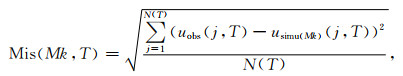
我们以真实高程模型下地形校正前后反演所得速度结构(图 8b、c)为基础,分别构建三维速度模型,计算合成地震记录,如图 5a红色与蓝色曲线所示.我们提取各自台站对间瑞利波频散曲线,以HS13-MZ14为例,如图 5b红色与蓝色曲线所示,记为usimu(Mk)(j, T).其中,j表示不同台站对,T表示不同周期,k=0, 1分别对应地形校正前后的速度模型.同时,将由真实模型(图 8a)所得的台站间瑞利波频散曲线记为uobs(j, T),如图 5b绿色曲线所示.我们定义误差函数:
|
(3) |
其中,N(T)表示不同周期的总频散曲线个数.式(3)反映了地形校正前后反演得到的速度结构与真实模型的差异程度,结果如图 5c所示.显然,地形校正后的结果要大大优于校正之前,校正后的频散曲线更加接近实际“观测”结果.
3 应用实例我们将上述地形校正方法应用于龙门山地区实际观测数据,也取得了良好的结果.与第2节理论测试中的建模工作类似,我们首先需要构建三维速度模型.与之前使用的理论初始速度模型不同,我们以由传统地震环境噪声面波成像方法得到的龙门山及周边地区S波速度结构(赵盼盼等,2015)为基础构建三维速度模型.然后采用相同的方法模拟三维波场,计算各台站间的合成地震记录.按照第1节所述校正处理流程,我们获得校正后的S波速度结构.图 9给出了研究区域内一条垂直剖面在地形校正前后的速度结构对比图.同时,该剖面的位置与Feng等(2016)的深反射剖面部分重合,因此我们将其结果与我们的结果比较印证.图 9b展示了由地震深反射剖面给出的映秀—北川断层(YBF)和灌县—江油断层(GJF)的壳内几何形态;图 9c展示了图 9a中s1剖面经地形校正后的S波速度结构;图 9d展示了该剖面未经地形校正的S波速度结构.相较于图 9d,图 9c中高角度铲形构造的断层形态很好的勾画出了地震环境噪声成像所呈现的地壳高速异常的外边缘;同时,余震分布与速度结构也有很好的吻合.由图 9的比较可以看出,经校正后的地震环境噪声成像得到的地壳S波速度结构是可靠的,而且其地形校正也是必要的.

|
图 9 地震环境噪声层析成像与地震深反射剖面的比较 (a)龙门山断裂带及其邻区地质背景;(b)地震深反射剖面(Feng et al., 2016).YBF:映秀—北川断裂;GJF:灌县—江油断裂;(c)地形校正后的s1剖面S波速度结构.WMF:汶川—茂县断裂;(d)未经地形校正的s1剖面S波速度结构.图(b)、(c)、(d)中红色实线表示汶川地震的破裂面;黑色实线表示未破裂滑脱面.图(c)、(d)中的实线红、黑线与图(b)中的一致;黑色的十字表示余震(陈九辉等,2009),剖面所示余震为距离剖面距离±5 km范围内的余震.图(b)、(c)、(d)的长度和深度的比例相同. Fig. 9 Comparison of the ambient noise tomographic imaging with the deep seismic reflection profile (a) Geological setting of the Longmenshan fault zone and adjacent regions; (b) The deep seismic reflection profile (Feng et al., 2016). YBF:Yingxiu-Beichuan fault. GJF:Guanxian-Jiangyou fault; (c) The S-wave velocity profile of s1 after topography correction. WMF: Wenchuan-Maoxian fault; (d) The S-wave velocity profile of s1 without topography correction. The solid red lines denote the rupture of the Wenchuan earthquake, and the solid black lines denote the un-ruptured slip plane in Fig.(b), (c), (d). The solid red and black lines in Fig.(c), (d) are coincident to those in the Fig.(b). The thin white lines depict the thin blue lines in the Fig.(b); the black crosses denote the aftershocks (Chen et al., 2009); the black crosses in Fig.(c), (d) denote the aftershocks in the range of ±5 km from the cross section. The scales of the Fig.(b), (c), (d) are the same for the length and the depth. |
对于在具有极端地形区域开展的成像研究工作,我们针对传统地震环境噪声面波成像方法,以地震波场的三维正演模拟为基础,提出了一种简单的地形校正方法.本文提出的地形和散射波场校正方法只需要进行一次三维正演,因而相比严格的基于数值计算的全波形反演方法和伴随成像方法,在计算效率上具有很大的优势.基于本文方法的理论测试及在实际数据上的应用都证明了该方法的有效性,同时也证明了地形校正的必要性.虽然我们的校正只是对地形影响的近似估计,但是对成像结果的改善是明显的.
Barmin M P, Ritwoller M H, Levshin A L. 2001. A fast and reliable method for surface wave tomography. Pure and Applied Geophysics, 158(8): 1351-1375. DOI:10.1007/PL00001225 |
Campillo M, Paul A. 2003. Long-Range correlations in the diffuse seismic coda. Science, 299(5606): 547-549. DOI:10.1126/science.1078551 |
Chen J H, Liu Q Y, Li S C, et al. 2009. Seismotectonic study by relocation of the Wenchuan MS8.0 earthquake sequence. Chinese Journal of Geophysics (in Chinese), 52(2): 390-397. DOI:10.1002/cjg2.1359 |
Chen M, Huang H, Yao H J, et al. 2014. Low wave speed zones in the crust beneath SE Tibet revealed by ambient noise adjoint tomography. Geophysical Research Letters, 41(2): 334-340. DOI:10.1002/2013GL058476 |
Chen M, Niu F L, Liu Q Y, et al. 2015. Multiparameter adjoint tomography of the crust and upper mantle beneath East Asia:1. Model construction and comparisons. Journal of Geophysical Research:Solid Earth, 120(3): 1762-1786. DOI:10.1002/2014JB011638 |
Chen Z H, Lou H, Meng X H, et al. 2014. 3D P-wave velocity structure of crust and upper mantle beneath Ordos Block and North China. Progress in Geophysics (in Chinese), 29(3): 999-1007. DOI:10.6038/pg20140303 |
Chu R S, Leng W, Helmberger D V, et al. 2013. Hidden hotspot track beneath the eastern United States. Nature Geoscience, 6(11): 963-966. DOI:10.1038/ngeo1949 |
Etienne V, Chaljub E, Virieux J, et al. 2010. An hp-adaptive discontinuous Galerkin finite-element method for 3-D elastic wave modelling. Geophysical Journal International, 183(2): 941-962. DOI:10.1111/j.1365-246X.2010.04764.x |
Fang L H, Wu J P, Lü Z Y. 2009. Rayleigh wave group velocity tomography from ambient seismic noise in North China. Chinese Journal of Geophysics (in Chinese), 52(3): 663-671. DOI:10.1002/cjg2.1388 |
Feng S Y, Zhang P Z, Liu B L, et al. 2016. Deep crustal deformation of the Longmen Shan, eastern margin of the Tibetan Plateau, from seismic reflection survey and Finite Element modelling. Journal of Geophysical Research:Solid Earth, 121(7): 767-787. DOI:10.1002/2015JB012352 |
Guo B, Chen J H, Liu Q Y, et al. 2019. Crustal structure beneath the Qilian Orogen Zone from multiscale seismic tomography. Earth and Planetary Physics, 3(3): 232-242. DOI:10.26464/epp2019025 |
Guo H L, Ding Z F, Xu X M. 2017. Upper mantle structure beneath the northern South-Nouth Seismic Zone from teleseismic traveltime data. Chinese Journal of Geophysics (in Chinese), 60(1): 86-97. DOI:10.6038/cjg20170108 |
Hermann R B, Ammon C J. 2002. Surface Waves, Receiver Function and Crustal Structure. St. Louis University.
|
Huang Z C, Wang P, Xu M J, et al. 2015. Mantle structure and dynamics beneath SE Tibet revealed by new seismic images. Earth and Planetary Science Letters, 411: 100-111. DOI:10.1016/j.epsl.2014.11.040 |
Komatitsch D, Martin R. 2007. An unsplit convolutional perfectly matched layer improved at grazing incidence for the seismic wave equation. Geophysics, 72(5): SM155-SM167. DOI:10.1190/1.2757586 |
Li H Y, Shen Y, Huang Z X, et al. 2013. The distribution of the mid-to-lower crustal low-velocity zone beneath the northeastern Tibetan Plateau revealed from ambient noise tomography. Journal of Geophysical Research:Solid Earth, 119(3): 1954-1970. DOI:10.1002/2013JB010374 |
Li Y, Yao H J, Liu Q Y, et al. 2010. Phase velocity array tomography of Rayleigh waves in western Sichuan from ambient seismic noise. Chinese Journal of Geophysics (in Chinese), 53(4): 842-852. DOI:10.3969/j.issn.0001-5733.2010.04.009 |
Lin F C, Li D Z, Clayton R W, et al. 2013. High-resolution 3D shallow crustal structure in Long Beach, California:Application of ambient noise tomography on a dense seismic array. Geophysics, 78(4): Q45-Q56. DOI:10.1190/GEO2012-0453.1 |
Liu Q, Gu Y J. 2012. Seismic imaging:From classical to adjoint tomography. Tectonophysics, 566-567: 31-66. DOI:10.1016/j.tecto.2012.07.006 |
Liu Y N, Niu F L, Chen M, et al. 2017a. 3-D crustal and uppermost mantle structure beneath NE China revealed by ambient noise adjoint tomography. Earth and Planetary Science Letters, 461: 20-29. DOI:10.1016/j.epsl.2016.12.029 |
Liu Z, Tian X B, Gao R, et al. 2017b. New images of the crustal structure beneath eastern Tibet from a high-density seismic array. Earth and Planetary Science Letters, 480: 33-41. DOI:10.1016/j.epsl.2017.09.048 |
Moschetti M P, Ritzwoller M H, Lin F, et al. 2009. Seismic evidence for widespread western-US deep-crustal deformation caused by extension. Nature, 464(7290): 885-889. DOI:10.1038/nature08951 |
Pang G H, Zhang L H, Liu T T, et al. 2014. An overview of development of ambient noise's application on crust and upper mantle's structure. Progress in Geophysics (in Chinese), 29(4): 1518-1525. DOI:10.6038/pg20140406 |
Pedersen H, Krüger F. 2007. Influence of the seismic noise characteristics on noise correlations in the Baltic shield. Geophysical Journal International, 168(1): 197-210. DOI:10.1111/j.1365-246X.2006.03177.x |
Qi C, Chen Q F, Chen Y. 2007. A new method for seismic imaging from ambient seismic noise. Progress in Geophysics (in Chinese), 22(3): 771-777. |
Ritzwoller M H, Lin F C, Shen W S. 2011. Ambient noise tomography with a large seismic array. Comptes Rendus Geoscience, 343(8-9): 558-570. DOI:10.1016/j.crte.2011.03.007 |
Roden J A, Gedney S D. 2000. Convolution PML (CPML):an efficient FDTD implementation of the CFS-PML for arbitrary media. Microwave and Optical Technology Letters, 27(5): 334-339. DOI:10.1002/1098-2760(20001205)27:5<334::AID-MOP14>3.0.CO;2-A |
Sabra K G, Gerstoft P, Roux P, et al. 2005a. Extracting time-domain Green's function estimates from ambient seismic noise. Geophysical Research Letters, 32(3): L03310. DOI:10.1029/2004GL021862 |
Sabra K G, Gerstoft P, Roux P, et al. 2005b. Surface wave tomography from microseisms in Southern California. Geophysical Research Letters, 32(14): L14311. DOI:10.1029/2005GL023155 |
Shapiro N M, Campillo M. 2004. Emergence of broadband Rayleigh waves from correlations of the ambient seismic noise. Geophysical Research Letters, 31(7): L07614. DOI:10.1029/2004GL019491 |
Shapiro N M, Campillo M, Stehly L, et al. 2005. High-resolution surface-wave tomography from ambient seismic noise. Science, 307(5715): 1615-1618. DOI:10.1126/science.1108339 |
Stehly L, Fry B, Campillo M, et al. 2009. Tomography of the Alpine region from observations of seismic ambient noise. Geophysical Journal International, 178(1): 338-350. DOI:10.1111/j.1365-246X.2009.04132.x |
Tape C H, Liu Q Y, Maggi A, et al. 2009. Adjoint tomography of the southern California crust. Science, 325(5943): 988-992. DOI:10.1126/science.1175298 |
Tape C H, Liu Q Y, Tromp J. 2007. Finite-frequency tomography using adjoint methods -methodology and examples using membrane surface waves. Geophysical Journal International, 168(3): 1105-1129. DOI:10.1111/j.1365-246X.2006.03191.x |
Tarantola A. 1984. Inversion of seismic reflection data in the acoustic approximation. Geophysics, 49(8): 1259-1266. DOI:10.1190/1.1441754 |
Tromp J, Tape C, Liu Q Y. 2005. Seismic tomography, adjoint methods, time reversal and banana-doughnut kernels. Geophysical Journal International, 160(1): 195-216. |
Wang S, Sun X L. 2019. Topography effect on ambient noise tomography using a dense seismic array. Earthquake Science, 32(5-6): 291-300. DOI:10.29382/eqs-2018-0291-9 |
Woodhouse J H, Dziewonski A M. 1984. Mapping the upper mantle:three-dimensional modeling of earth structure by inversion of seismic waveforms. Journal of Geophysical Research:Solid Earth, 89(B7): 5953-5986. DOI:10.1029/JB089iB07p05953 |
Xu M J, Huang H, Huang Z C, et al. 2018. Insight into the subducted indian slab and origin of the tengchong volcano in se Tibet from receiver function analysis. Earth and Planetary Science Letters, 482: 567-579. DOI:10.1016/j.epsl.2017.11.048 |
Yao H J, Beghein C, Van Der Hilst R D. 2008. Surface wave array tomography in SE Tibet from ambient seismic noise and two-station analysis-Ⅱ. Crustal and upper-mantle structure. Geophysical Journal International, 173(1): 205-219. DOI:10.1111/j.1365-246X.2007.03696.x |
Yao H J, Van Der Hilst R D, De Hoop M V. 2006. Surface-wave array tomography in SE Tibet from ambient seismic noise and two-station analysis-I. Phase velocity maps. Geophysical Journal International, 166(2): 732-744. DOI:10.1111/j.1365-246X.2006.03028.x |
Zhao P P, Chen J H, Liu Q Y, et al. 2015. Fine structure of middle and upper crust of the Longmenshan Fault zone from short period seismic ambient noise. Chinese Journal of Geophysics (in Chinese), 58(11): 4018-4030. |
Zheng C, Ding Z F, Song X D. 2018. Joint inversion of surface wave dispersion and receiver functions for crustal and uppermost mantle structure beneath the northern north-south seismic zone. Chinese Journal of Geophysics (in Chinese), 61(4): 1211-1224. |
Zhong S J, Wu J P, Fang L H, et al. 2017. Surface wave Eikonal tomography in and around the northeastern margin of the Tibetan plateau. Chinese Journal of Geophysics (in Chinese), 60(6): 2304-2314. |
Zhu H J, Bozdag E, Peter D, et al. 2012. Structure of the European upper mantle revealed by adjoint tomography. Nature Geoscience, 5(7): 493-498. DOI:10.1038/ngeo1501 |
陈九辉, 刘启元, 李顺成, 等. 2009. 汶川MS8.0地震余震序列重新定位及其地震构造研究. 地球物理学报, 52(2): 390-397. |
陈兆辉, 楼海, 孟小红, 等. 2014. 鄂尔多斯块体-华北地区地壳上地幔P波三维速度结构. 地球物理学进展, 29(3): 999-1007. DOI:10.6038/pg20140303 |
房立华, 吴建平, 吕作勇. 2009. 华北地区基于噪声的瑞利面波群速度层析成像. 地球物理学报, 52(3): 663-671. |
郭慧丽, 丁志峰, 徐小明. 2017. 南北地震带北段的远震P波层析成像研究. 地球物理学报, 60(1): 86-97. DOI:10.6038/cjg20170108 |
李昱, 姚华建, 刘启元, 等. 2010. 川西地区台阵环境噪声瑞利波相速度层析成像. 地球物理学报, 53(4): 842-852. DOI:10.3969/j.issn.0001-5733.2010.04.009 |
庞广华, 张林行, 刘婷婷, 等. 2014. 利用背景噪声研究壳幔结构发展综述. 地球物理学进展, 29(4): 1518-1525. DOI:10.6038/pg20140406 |
齐诚, 陈棋福, 陈颙. 2007. 利用背景噪声进行地震成像的新方法. 地球物理学进展, 22(3): 771-777. |
赵盼盼, 陈九辉, 刘启元, 等. 2015. 龙门山断裂带中上地壳速度结构的短周期环境噪声成像. 地球物理学报, 58(11): 4018-4030. DOI:10.6038/cjg20151111 |
郑晨, 丁志峰, 宋晓东. 2018. 面波频散与接收函数联合反演南北地震带北段壳幔速度结. 地球物理学报, 61(4): 1211-1224. DOI:10.6038/cjg2018L0443 |
钟世军, 吴建平, 房立华, 等. 2017. 青藏高原东北缘及周边地区基于程函方程的面波层析成像. 地球物理学报, 60(6): 2304-2314. DOI:10.6038/cjg20170622 |