 2019, Vol. 62


2. 成都理工大学数学地质四川省重点实验室, 成都 610059;
3. 安徽万泰地球物理技术有限公司, 合肥 230026
2. Geomathematics Key Laboratory of Sichuan Province, Chengdu University of Technology, Chengdu 610059, China;
3. Anhui Wantai Geophysical Technology Co. Ltd., Hefei 230026, China
在工业领域里,人工加压注水方法已广泛应用于采油、采气、采盐及废水处理等方面.在油气开采中,人们普遍采用注水压裂的方法来提高油气产量.伴随着水力压裂裂缝的产生会发生一系列微弱的地震事件,其震级通常在0级以下.通过对这些微地震事件进行监测,得到震源位置等参数,可实现实时监测裂缝发育状况的目的(Warpinski et al., 1997; Maxwell et al., 2002; Rutledge and Phillips, 2003).然而,如果压裂施工区处于某些特定的地质环境中,注水过程可能引发较大的地震.这些地震的震级一般在2~4级,由于震源深度较浅,对地表建筑物及人类活动会产生较大破坏作用(王小龙等, 2011; 张致伟等, 2012; Ellsworth, 2013).对诱发地震及微地震进行监测的主要目的是获取震源参数,包括震源位置、发震时刻、释放能量大小和震源机制等.通过地震的时空分布规律,可以了解裂缝的分布范围,研究诱发地震与注水过程之间的关联性.通过震源机制解,可以确定裂缝产生的力学机制和描述裂缝的破裂过程,进而对工区的地应力状态进行分析,这对指导后期压裂井部署及水力压裂施工具有重要意义.
作为地震学领域的热点问题,震源机制理论和方法研究一直受到国内外专家学者的关注.震源机制解可以用矩张量的形式表示;如果震源为剪切源(又称双力偶源),在这种情况下震源机制以断层平面解的形式表示,是一般矩张量模型的一种特殊形式.目前,在确定震源机制解时经常采用的方法包括P波初动极性法、纵横波振幅比法和全波形方法,其中P波初动极性法和振幅比法常用于求取断层平面解,在求取矩张量时多采用全波形方法.P波初动极性法是最简单、常用的快速求取震源机制解的方法.该方法基本原理为通过比较观测的P波初动极性与理论P波极性,选取拟合差最小的一组解为真实的震源机制解(Reasenberg and Oppenheimer, 1985);Hardebeck和Shearer(2002)改进了传统的利用P波初动极性求取震源机制解的方法,将速度模型及震源位置误差对P波极性的影响考虑了进来;Nakamura(2002, 2004)将S波极性也考虑进来,加强对解的约束.Kisslinger(Kisslinger, 1980; Kisslinger et al., 1981)研究发现纵横波振幅比对于震源机制解的确定具有很好的约束作用,并在此基础上提出了利用纵横波振幅比确定震源机制解的方法;Snoke等(1984)提出综合利用P波、SV波、SH波之间的振幅比信息确定震源机制解的方法;Hardebeck和Shearer(2003)在原有的P波初动极性法基础上加入SV/P振幅比约束来更加准确地求取震源机制解.
自20世纪50年代起,一些学者就试图采用全波形数据来确定震源机制解.鉴于地震记录与矩张量之间的线性关系,Stump和Johnson(1977)采用最小二乘方法反演震源矩张量;Dziewonski等(1981)提出联合反演矩张量与震源位置的方法;Šílený等(1992)将介质模型对矩张量反演结果的影响考虑进来;Dreger和Helmberger(1993)使用近震宽频带数据,采用全波形匹配的方法反演得到震源机制解.作为目前应用最广的一类全波形反演方法,Zhao和Helmberger(1994)、Zhu和Helmberger(1996)提出并发展了CAP、gCAP等方法.该方法将地震波形记录P波和S波部分分开进行拟合,并将不同的权重赋给它们,最后利用网格搜索方法得到震源机制解.Tan和Helmberger(2007)采用CAP方法研究了中、小型地震(ML≤3.5)的震源机制,取得了良好的应用效果.在进行波形拟合时我们通常将P波和S波分开并做归一化处理,这样做的目的是为了消除由于速度模型误差引入的到时误差,然而这样做会忽略波形的振幅信息;另外,对于初动起跳不明显的信号,采用全波形拟合容易出现理论记录的P波初动极性与实际记录不一致的情况.Li等(2011a, b)综合P波初动极性、纵横波振幅比及波形信息构建目标函数,采用网格搜索方法求取震源机制解,并成功应用于井下和地面诱发地震监测数据.但是,该方法存在目标函数中各项之间权重难以优化选择的问题;另外,Li等(2011a, b)采用该方法反演剪切源的断层平面解,在确定矩张量方面还未有应用.
本文在借鉴Li等(2011a, b)方法的基础上,首先研究了P波初动极性和纵横波振幅比对于震源机制解的约束作用;之后提出了一种新的震源机制反演方法,并采用新方法确定国内某页岩气田诱发地震的震源机制.
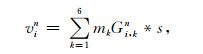
1 基于全波形匹配的震源机制反演方法采用全波形匹配的方法确定震源机制,首先需要正演计算理论地震记录.根据Aki和Richards(1980),地震记录与矩张量之间满足如下线性关系:
|
(1) |
其中vin(i=1, 2, 3; n=1, 2, …, N)表示理论地震记录,mk(k=1, 2, …, 6)表示矩张量的六个独立元素,Gi, kn为格林函数,s为震源时间函数,*表示卷积运算.格林函数Gi, kn可认为是模型介质的单位脉冲响应,它描述了介质对地震波传播效应的影响.在计算理论记录前,需要事先根据震源位置和速度模型建立格林函数库.本文采用Bouchon(1981)提出的离散波数法计算格林函数库.
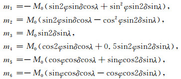
若对震源作剪切源(双力偶源)假设,在该假设条件下震源机制可以用断层平面解表示,且断层面三个角度(即方位角φ、倾角δ和滑动角λ)与矩张量元素mk存在如下关系:
|
(2) |
其中M0为标量地震矩(本文方法不对M0进行反演,在反演矩张量时将M0的值设为1).利用(2)式可将断层面的三个角度转换为矩张量元素,再代入(1)式计算理论地震记录,即可实现对断层平面解的反演.
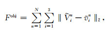
为了定量描述理论地震记录与实际记录之间波形匹配程度,通常采用二者的L2范数作为目标函数,即
|
(3) |
其中

|
(4) |
其中P(Vin)、P(vin)分别为实际和理论地震记录的P波初动极性,R(Vin)、R(vin)分别为实际和理论地震记录的纵横波振幅比,f[P(Vin), P(vin)]、h[R(Vin), R(vin)]分别表示求P波初动极性和纵横波振幅比的拟合差,⊗表示互相关运算,α1~α4为权值系数.相比于(3)式,(4)式中加入了P波初动极性和纵横波振幅比作为约束(即第三项和第四项),在拟合波形的同时实现对二者的最佳匹配.
本文首先采用合成数据检验加入P波初动极性和纵横波振幅比的新目标函数(即(4)式)对于震源机制解的约束作用.在该算例中,我们对合成数据的断层平面解和矩张量均进行反演.在反演断层平面解时,由于断层面的方位角φ、倾角δ和滑动角λ与理论地震记录vin之间关系为非线性,通常采用全局优化算法对其进行求解.网格搜索法是最常用的一种全局优化算法,该算法具有原理简单、实现方便以及能够得到全局极值点等优势,然而该算法的效率会随着反演参数的增多而显著下降.由于在反演矩张量时需要对矩张量的六个独立元素进行搜索,采用传统网格搜索法效率较低,因此,本文采用邻域最优化算法对矩张量以及断层平面解进行反演.
邻域算法是一种直接搜索算法,与其他全局优化算法(例如模拟退火算法和遗传算法)相比,邻域算法仅根据先前产生的模型来决定后续模型,具有更强的自适应性和更少的调节参数(Sambridge, 1999).邻域算法的基本元素为Voronoi单元.Voronoi单元定义为每一个点的相邻区域,在该区域内任意一点到其定义点的距离最短.通过将每个Voronoi单元中对应的目标函数值设为常数,可得到目标函数的一个近似面,称为NA面.NA面提供了对参数空间中不规则分布点的简单非光滑插值,图 1显示了对于一个二维参数空间得到的不同迭代次数下的NA面示意图.由该图可知Voronoi单元的大小和采样点的密度成反比,即在样点分布密集的区域,Voronoi单元较小;而在样点分布稀疏的区域,Voronoi单元较大.Voronoi单元的这一特征表明每一个单元的大小和形状完全由样本自身决定.假设通过某种方法可以产生新的样本,这些新样本能够局部地改变Voronoi单元的大小,从而改善NA面的局部分辨率,实现对参数空间的最佳区域进行优先搜索.邻域算法的具体步骤为:

|
图 1 NA面示意图 图中黑色圆点表示不同迭代次数产生的所有采样点.(a)迭代1次;(b)迭代2次;(c)迭代3次;(d)迭代4次. Fig. 1 Diagrams of the NA surface The black dots denote all samples generated after different iteration steps. (a) After 1 iteration step; (b) After 2 iteration steps; (c) After 3 iteration steps; (d) After 4 iteration steps. |
(1) 在参数空间内随机产生ns个初始模型;
(2) 计算每个新模型的目标函数值;
(3) 选取目标函数值最小的nr个模型;
(4) 在nr个模型所对应的Voronoi单元中再随机产生ns个新模型(即每个Voronoi单元产生ns/nr个新模型);
(5) 返回步骤(2),直到达到最大迭代次数.
图 2为合成数据的观测系统示意图.震源位于[9.5, 11.5, 7.0]km,其震源机制如图中沙滩球所示(具体参数见表 1).计算格林函数所采用的速度模型如图 3所示.图 4a为根据(1)式及表 1中震源参数计算得到的合成数据波形(垂直分量),其中添加了约80%的随机噪声.在反演震源机制时,我们首先采用一个通带为[5, 15]Hz的带通滤波器对合成数据进行滤波,滤波后的波形如图 4b所示;之后,分别采用(3)式和(4)式作为目标函数对滤波后的数据进行反演.在采用(4)式反演时选取的权值系数分别为α1=0.3, α2=1, α3=0.3, α4=0.02.图 5和图 6分别显示了采用(3)式和(4)式得到的反演结果.通过对比发现,(4)式得到的反演结果更加接近真实的震源机制.比较反演结果对应的理论记录与合成数据的匹配程度发现,(3)式得到的反演结果与合成数据的平均波形相似度(即二者归一化互相关函数最大值)为0.7570(断层平面解反演)和0.7720(矩张量反演),优于(4)式的反演结果(即0.7296和0.7393),但在P波初动极性和纵横波振幅比方面则与合成数据存在明显误差.相比较而言,(4)式的反演结果虽然在拟合波形方面存在一定误差,但其P波初动极性与纵横波振幅比与合成数据具有很好的一致性.由于该算例所采用的合成数据包含噪声,会导致反演结果的理论波形与合成数据无法完全拟合,在该情况下采用P波初动极性和纵横波振幅比对解进行约束则可以有效降低噪声对反演结果的影响.

|
图 2 观测系统示意图 图中蓝色三角形表示台站位置,红色星号表示合成数据的震源位置,沙滩球表示合成数据震源机制. Fig. 2 Diagram of the monitoring system The blue triangles denote the stations, the red star denotes the source location of the synthetic data, and the beach ball denotesthe source mechanism of the data. |
|
|
表 1 合成数据震源参数 Table 1 Source parameters of the synthetic data |

|
图 3 速度模型 Fig. 3 Velocity model |

|
图 4 合成数据波形 图中竖线表示理论计算P波(实线)和S波(虚线)到时. (a)滤波前;(b)滤波后. Fig. 4 Waveforms of the synthetic data The vertical bars denote the theoretical P (solid line) and S (dashed line) wave arrival times.(a) Before filtering; (b) After filtering. |

|
图 5 采用(3)式作为目标函数反演得到的震源机制解 图中左侧沙滩球表示反演结果,右侧子图中的蓝色曲线表示合成数据波形,红色曲线表示反演结果对应的理论记录波形,右上角数字表示合成数据与理论记录的波形相似度(即二者归一化互相关函数最大值),右下角符号或数字表示合成数据(左)与理论记录(右)的P波初动极性或纵横波振幅比. (a)断层平面解;(b)矩张量. Fig. 5 Inverted source mechanism solutions using equation (3) The beach balls at the left hand denote the solutions, the blue lines in the sub-plots at the right hand denote the waveforms of the synthetic data, the red lines denote the waveforms of the theoretical seismograms of the solutions, the numbers at the upper right corner denote the degrees of waveform similarity between the two data (i.e. the maximum value of normalized cross-correlation function), the signs or the numbers at the lower right corner denote the P wave first motion polarities or S/P amplitude ratios of the synthetic data (left) and the theoretical seismograms (right).(a) Fault plane solution; (b) Moment tensor. |

|
图 6 采用(4)式作为目标函数反演得到的震源机制解 图中左侧沙滩球表示反演结果,右侧子图中的蓝色曲线表示合成数据波形,红色曲线表示反演结果对应的理论记录波形,右上角数字表示合成数据与理论记录的波形相似度(即二者归一化互相关函数最大值),右下角符号或数字表示合成数据(左)与理论记录(右)的P波初动极性或纵横波振幅比. (a)断层平面解;(b)矩张量. Fig. 6 Inverted source mechanism solutions using equation (4) The beach balls at the left hand denote the solutions, the blue lines in the sub-plots at the right hand denote the waveforms of the synthetic data, the red lines denote the waveforms of the theoretical seismograms of the solutions, the numbers at the upper right corner denote the degrees of waveform similarity between the two data (i.e. the maximum value of normalized cross-correlation function), the signs or the numbers at the lower right corner denote the P wave first motion polarities or S/P amplitude ratios of the synthetic data (left) and the theoretical seismograms (right).(a) Fault plane solution; (b) Moment tensor. |
采用(4)式作为目标函数反演震源机制时,需要确定权值系数α1~α4.在选择α1~α4时遵循的原则为(4)式中每一项所占的比重应大致相当.然而,对于不同实际数据,我们需要选择不同的权值系数,而在选择权值系数时,往往需要经过多次试验才能得到一组最优的值.为了避免权值系数选择问题,本文采用一种分级优化策略来同时优化多个目标函数(例如(4)式中的每一项均可认为是独立的目标函数)确定震源机制解.
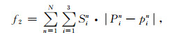
邻域算法的一个重要特性是该算法仅利用目标函数值的排序(即相对大小)搜索参数空间,而不需要目标函数的绝对值.根据这一特性,我们发展了一种新的震源机制反演方法,该方法的基本原理为采用不同的目标函数分级排除部分匹配度较差的解(Tan et al., 2018).新方法采用的目标函数包括:

|
(5) |
|
(6) |

|
(7) |
其中

(1) 在参数空间内随机产生ns个初始解;
(2) 根据(5)—(7)式计算每个新生成的解的目标函数值f1、f2和f3;
(3) 根据目标函数值f1对目前已经产生的所有nall个解(包括之前迭代步中产生的解)进行从大到小排序,剔除(nall-nr)/3个目标函数值最大的解;
(4) 根据目标函数值f2对剩余解进行从大到小排序,剔除(nall-nr)/3个目标函数值最大的解;
(5) 根据目标函数值f3对剩余解进行从大到小排序,剔除(nall-nr)/3个目标函数值最大的解;
(6) 在剩余的nr个解所对应的Voronoi单元中再随机产生ns个新解;
(7) 返回步骤(2),直到达到最大迭代次数.
为了检验新方法的应用效果,我们采用与第1节相同的合成数据对方法进行测试.测试结果如图 7所示,可以看到反演结果与真实震源机制(表 1)具有很好的一致性,且反演结果的理论P波初动极性和纵横波振幅比与合成数据也基本一致.与Li等(2011a, b)方法相比,新方法无需确定权值系数α1~α4,对于不同数据具有更强的适用性.图 8显示了采用新方法搜索断层平面解(图 8a)和矩张量的过程(图 8b),可以看到随着迭代的进行断层平面解(即方位角φ、倾角δ、滑动角λ)和矩张量参数(即m1、m2、m3、m4、m5、m6)均趋于收敛,目标函数值(即f1、f2、f3)也逐渐减小,表明新方法能够搜索到全局最优解.需要注意的是,图 8a中方位角φ、倾角δ、滑动角λ均收敛到两组解,它们分别对应于表 1中节面I和II;另外,目标函数f1和f3并未减小至0则是由于合成数据中存在随机噪声造成的.

|
图 7 采用新方法反演得到的震源机制解 图中左侧沙滩球表示反演结果,右侧子图中的蓝色曲线表示合成数据波形,红色曲线表示反演结果对应的理论记录波形,右上角数字表示合成数据与理论记录的波形相似度(即二者归一化互相关函数最大值),右下角符号或数字表示合成数据(左)与理论记录(右)的P波初动极性或纵横波振幅比. (a)断层平面解;(b)矩张量. Fig. 7 Inverted source mechanism solutions using the new method The beach balls at the left hand denote the solutions, the blue lines in the sub-plots at the right hand denote the waveforms of the synthetic data, the red lines denote the waveforms of the theoretical seismograms of the solutions, the numbers at the upper right corner denote the degrees of waveform similarity between the two data (i.e. the maximum value of normalized cross-correlation function), the signs or the numbers at the lower right corner denote the P wave first motion polarities or S/P amplitude ratios of the synthetic data (left) and the theoretical seismograms (right). (a) Fault plane solution; (b) Moment tensor. |

|
图 8 采用新方法搜索合成数据震源机制解过程,每次迭代步产生1000组新解 (a)断层平面解;(b)矩张量. Fig. 8 Illustration of the search process for source mechanism of the synthetic data by the new method. 1000 new solutions are generated in each iteration step (a) Fault plane solution; (b) Moment tensor. |
如果地震事件的初至起跳不明显会造成P波初动极性难以准确判断,因此,在处理实际数据时我们仅采用部分能够准确判定的P波初动极性用于反演;另外,低信噪比会造成地震事件的纵横波振幅比降低.由于在计算目标函数(6)式和(7)式时,我们采用的是未经滤波处理的实际记录,而在计算(5)式时采用滤波后的记录,因此,实际记录中的噪声对目标函数f2和f3有较大影响.为了降低噪声对反演结果的影响,可以通过调节算法每次迭代中根据不同目标函数剔除的解的个数来实现.例如,对于低信噪比事件我们希望反演解能够更好拟合地震波形,则在步骤(3)中可以剔除更多的(大于(nall-nr)/3)目标函数值f1较大的解,从而保证每次迭代中更多的能够较好拟合地震波形的解被保留下来.
震源机制反演最大的问题在于区域速度模型难以准确获取.为了测试速度模型误差对震源机制解精度的影响,我们进行了4组Monte-Carlo测试.在每组测试中我们对图 3中每一层的P波和S波速度值进行了随机扰动(地层界面深度保持不变),产生了100组经过扰动的模型.4组Monte-Carlo测试的最大速度扰动量分别为±5%、±10%、±15%和±20%.我们采用扰动后的速度模型反演图 4中合成数据的震源机制解,结果如图 9a所示,可以看到随着模型扰动量的增大,震源机制解误差也逐渐增大.对于本文监测目标区,20%的速度扰动量通常被认为是一个合理的误差范围,由图 9a可知震源机制反演结果误差在可接受的范围内.

|
图 9 速度模型或(和)震源位置存在误差时震源机制解对比 图中红色沙滩球表示真实断层平面解(表 1),绿色曲线表示反演得到的断层平面解;T-k图中红色圆点表示真实矩张量(表 1),绿色圆点表示反演得到的矩张量;σv和σs分别表示速度模型和震源深度的最大扰动量. (a)仅速度模型存在误差时的解;(b)仅震源深度存在误差时的解;(c)速度模型和震源深度均存在误差时的解. Fig. 9 Comparison of the inverted source mechanism solutions with errors in the velocity model or/and source location The red beach ball denotes the true fault plane solution (Table 1), and the green lines in the beach ball denote the inverted fault plane solutions. The red dot in the T-k plots denotes the true moment tensor (Table 1), and the green dots denote the inverted moment tensors. σv and σs are the maximum perturbations applied to the velocity model and source depth. (a) Inverted solutions with errors only in the velocity model; (b) Inverted solutions with errors only in the source depth; (c) Inverted solutions with errors in both velocity model and source depth. |
除速度模型外,震源定位误差也是影响震源机制解精度的一个重要因素.实际数据定位误差通常表现为震源深度上误差较大,因此,许多震源机制反演方法在确定震源机制的同时对震源深度也进行确定(例如Zhao and Helmberger, 1994; Zhu and Helmberger, 1996).在本文中,我们同样研究了震源定位误差对于震源机制解的影响.采用的研究方法与前面类似,分别进行了4组Monte-Carlo测试,在每组测试中我们对真实震源深度(即7.0 km)进行了100次随机扰动,最大扰动量分别为±0.5 km、±1.0 km、±1.5 km和±2.0 km.根据扰动后的震源深度反演得到合成数据的震源机制解如图 9b所示,可以看到反演结果误差同样随震源深度误差增大而增大.相比较而言,震源定位误差对震源机制解精度的影响小于速度模型误差的影响,该结论与Šílený(2009)得到的结论一致.
在处理实际数据时,速度模型和震源位置往往同时存在误差(速度模型误差也是造成震源定位误差的主要因素之一),因此,我们也测试了当速度模型与震源位置同时存在误差时的反演结果(如图 9c所示),发现该情况下震源机制解误差大于二者之一(速度模型或震源位置)存在误差时的结果.为了减小误差对反演结果精度的影响,我们借鉴前人方法的思路,即同时反演震源机制与震源位置(Zhao and Helmberger, 1994; Zhu and Helmberger, 1996),具体做法为等间隔选择不同的震源深度,采用本文方法首先反演得到各个深度对应的震源机制解;然后,选择波形拟合差最小的深度为真实震源深度,其对应的震源机制解为最终反演结果.在下面实际数据测试中,我们采用该方法同时确定震源机制与震源深度.
3 实际诱发地震震源机制反演本文将新方法用于确定国内某页岩气开采区诱发地震震源机制.监测目标区位于四川盆地南缘,属山区地带,总体地势呈南高北低,海拔在600~1000 m之间.区内表面风化剥蚀严重,出露的地层较为齐全,从寒武纪中上统娄山关群至侏罗系上统遂宁组,除泥盆系和石炭系缺失外,各时代地层均有出露.区内下志留统龙马溪组为主要页岩气储层,其有效页岩厚度为20~60 m,埋深在2~4.5 km左右(杨洋, 2016).监测区域内历史地震活动较为稳定,1996—2014年间仅发生过39次震级在ML2.0以上的地震;然而到2018年7月已发生震级大于ML2.0地震106次(据国家地震科学数据共享中心,http://data.earthquake.cn/).有研究指出地震活动的增加与该地区实施水力压裂开采页岩气有关(Lei et al., 2017).从2017年2月开始,我们在监测目标区内布设了10个流动台站(台站位置如图 1所示),用于监测与该地区页岩气开采有关的地震活动.本文使用的数据为2017年2月至2018年1月的监测数据.经过前期处理,识别出了约7300个地震事件,这些事件的震级主要集中在Mw0~2.5.通过采用双差成像-定位算法(Zhang and Thurber, 2003, 2006),获得了这些事件的精确震源位置,如图 10所示.

|
图 10 诱发地震震源位置 Fig. 10 Source locations of the induced seismicity |
我们从识别出的地震事件中选取了一个信噪比较高的事件,该事件的震源位置如图 10中红色星号所示.首先采用5~15 Hz的带通滤波器对该事件进行滤波,滤波前后的地震记录如图 11所示.由于台站的水平分量方位未知,在反演该事件震源机制解时我们只采用垂直分量记录;另外,该事件中S05和S10两个台站的记录由于信噪比较低以及数据缺失,在反演时并未使用.采用新方法得到该事件的震源机制解(包括断层平面解和矩张量)如图 12a所示.断层平面解结果表明该事件的破裂类型为走滑破裂,矩张量反演结果表明该事件以剪切成分为主,这与许多学者提出水力压裂诱发地震的震源机制为剪切破裂(或以剪切成分为主)是一致的(Jost et al., 1998; Dahm et al., 1999; Horálek et al., 2010; Song and Toksöz, 2011; Wang et al., 2016; Pesicek et al., 2016).通过比较实际数据波形与反演结果理论波形可知二者能够较好拟合;另外,从实际数据中提取出的P波初动极性(S03、S06和S07台站记录的P波初动极性无法准确确定)和纵横波振幅比与理论记录也能够较好吻合,表明得到的震源机制解较为可靠.

|
图 11 测试事件垂直分量波形记录 图中竖线表示手动拾取的P波(实线)和S波(虚线)到时,虚线方框表示带通滤波器的通带范围(5~15 Hz). (a)滤波前记录;(b)记录的频谱;(c)滤波后记录. Fig. 11 Vertical component waveforms of the testing event The vertical bars denote the manually picked P (solid line) and S (dashed line) wave arrival times, the dashed box denotes the passband of the band-pass filter (5~15 Hz). (a) Waveforms before filtering; (b) Spectra of the waveforms before filtering; (c) Waveforms after filtering. |

|
图 12 测试事件震源机制反演结果 图中左侧沙滩球表示反演断层平面解或矩张量,右侧子图中的蓝色曲线表示实际数据波形,红色曲线表示反演结果对应的理论记录波形,右上角数字表示实际数据与理论记录的波形相似度(即二者归一化互相关函数最大值),右下角符号或数字表示实际数据(左)与理论记录(右)的P波初动极性或纵横波振幅比. (a)新方法得到的反演结果;(b)利用(3)式作为目标函数得到的反演结果;(c)利用(4)式作为目标函数得到的反演结果. Fig. 12 Inverted source mechanism solutions of the testing event The beach balls at the left hand denote the inverted fault plane solutions or the moment tensors, the blue lines in the sub-plots at the right hand denote the waveforms of the real data, the red lines denote the waveforms of the theoretical seismograms of the solutions, the numbers at the upper right corner denote the degrees of waveform similarity between the two data (i.e. the maximum value of normalized cross-correlation function), the signs or the numbers at the lower right corner denote the P wave first motion polarities or S/P amplitude ratios of the real data (left) and the theoretical seismograms (right). (a) Inversion results using the new method; (b) Inversion results using equation (3);(c) Inversion results using equation (4). |
为了对比,我们分别采用第2节中(3)式和(4)式作为目标函数对图 11中地震事件进行了反演,结果如图 12b和12c所示.通过对比图 12a和12b发现,采用(3)式作为目标函数反演得到的震源机制解虽然可以更好地拟合实际地震记录,但其P波初动极性和纵横波振幅比与实际记录存在明显误差.相比较而言,采用(4)式作为目标函数在拟合波形的同时对P波初动极性与纵横波振幅比也具有较好的约束(图 12c),其反演结果与新方法得到的结果基本一致.
我们选择了10个具有不同震源位置的典型诱发地震事件,采用新方法反演得到这些事件的震源机制解如图 13所示(波形对比见附录).由反演结果可知,这些地震事件多为走滑破裂或具有明显的走滑成分,走滑破裂占据主导表明该地区的最大水平主应力σHmax大于垂直主应力σV(Zoback, 2007).前人研究结果表明,该地区最大水平主应力方向为北偏东100°~115°(Lei et al., 2017).由图 13可知,对于部分地震事件(例如#01131、#05422等),其震源机制解P轴与最大水平主应力方向接近,表明这些地震的发生受区域构造应力场控制;另外,部分事件的P轴方向与最大水平主应力方向近似垂直(例如#00438、#05124等),表明附近水力压裂施工导致局部地应力场发生变化.需要注意的是,由于速度模型以及震源定位误差也可能导致部分震源机制解存在一定误差.

|
图 13 典型诱发地震事件震源机制反演结果 Fig. 13 Inverted source mechanism solutions of typical induced events with different source locations |
通过对比发现,断层平面解结果的可靠性好于矩张量结果.这是由于在反演断层平面解时只需要搜索三个参数(即方位角φ、倾角δ和滑动角λ),而反演矩张量时需要搜索六个参数(即m1、m2、m3、m4、m5、m6),模型参数的增多会造成反演结果存在较大的不确定性(即存在多组解能够拟合观测数据)(Stierle et al., 2014).为了提高矩张量反演结果的可靠性,可以利用某些先验信息对反演进行约束,例如Li等(2016)提出了一种利用双力偶震源机制解来约束矩张量反演的方法.借鉴该方法原理,我们对本文提出方法进行了改进,即加入一个新的目标函数将矩张量解限定在已求得断层平面解的附近.我们选取图 13中的一个地震事件对改进方法进行了测试,测试结果表明改进方法得到的矩张量结果与断层平面解具有更好的一致性(图 14).

|
图 14 图 13中事件#05250震源机制反演结果对比 (a)断层平面解;(b)无约束矩张量反演结果;(c)采用断层平面解约束的矩张量反演结果. Fig. 14 Comparison of the inverted source mechanism solutions of Event#05250 in Fig. 13 (a) Fault plane solution; (b) Unconstrained moment tensor solution; (c) Moment tensor solution using the fault plane solution as constraint. |
本文采用全波形匹配的方法求取地震事件的震源机制解,在拟合波形的同时对实际数据P波初动极性和纵横波振幅比也进行匹配.合成数据测试结果表明全波形匹配方法对震源机制解具有更好的约束,反演结果更加接近真实值.在全波形匹配的基础上,本文发展了一种基于邻域算法分级优化确定震源机制解的方法.合成数据测试结果表明新方法能够有效解决目前已有方法中存在的权值系数选择问题,具有更强的适用性.本文采用新方法确定了国内某页岩气田诱发地震的震源机制,反演结果表明该地区诱发地震的震源类型以走滑破裂为主,表明该地区最大水平主应力大于垂直主应力.另外,实际数据测试结果表明采用断层平面解对矩张量反演进行约束能够提高反演结果的可靠性.
附录图 13中10个地震事件(红色星号)的震源机制反演结果及波形对比如图 A1所示.

|
图 A1 图 13中地震事件震源机制反演结果 图中左侧沙滩球表示反演断层平面解或矩张量,右侧子图中的蓝色曲线表示实际数据波形,红色曲线表示反演结果对应的理论记录波形,右上角数字表示实际数据与理论记录的波形相似度(即二者归一化互相关函数最大值),右下角符号或数字表示实际数据(左)与理论记录(右)的P波初动极性或纵横波振幅比. Fig. A1 Inverted source mechanism solutions of the typical events in Fig. 13 The beach balls at the left hand denote the inverted fault plane solutions or the moment tensors, the blue lines in the sub-plots at the right hand denote the waveforms of the real data, the red lines denote the waveforms of the theoretical seismograms of the solutions, the numbers at the upper right corner denote the degrees of waveform similarity between the two data (i.e. the maximum value of normalized cross-correlation function), the signs or the numbers at the lower right corner denote the P wave first motion polarities or S/P amplitude ratios of the real data (left) and the theoretical seismograms (right). |
Aki K, Richards P. 1980. Quantitative seismology:Theory and Methods. London: W.H. Freeman and Co.
|
Bouchon M. 1981. A simple method to calculate Green's functions for elastic layered media. Bulletin of the Seismological Society of America, 71(4): 959-971. |
Dahm T, Manthei G, Eisenblätter J. 1999. Automated moment tensor inversion to estimate source mechanisms of hydraulically induced micro-seismicity in salt rock. Tectonophysics, 306(1): 1-17. DOI:10.1016/S0040-1951(99)00041-4 |
Dreger D S, Helmberger D V. 1993. Determination of source parameters at regional distances with three-component sparse network data. Journal of Geophysical Research:Solid Earth, 98(B5): 8107-8125. DOI:10.1029/93JB00023 |
Dziewonski A M, Chou T A, Woodhouse J H. 1981. Determination of earthquake source parameters from waveform data for studies of global and regional seismicity. Journal of Geophysical Research:Solid Earth, 86(B4): 2825-2852. DOI:10.1029/JB086iB04p02825 |
Ellsworth W L. 2013. Injection-induced earthquakes. Science, 341(6142): 1225942. DOI:10.1126/science.1225942 |
Hardebeck J L, Shearer P M. 2002. A new method for determining first-motion focal mechanisms. Bulletin of the Seismological Society of America, 92(6): 2264-2276. DOI:10.1785/0120010200 |
Hardebeck J L, Shearer P M. 2003. Using S/P amplitude ratios to constrain the focal mechanisms of small earthquakes. Bulletin of the Seismological Society of America, 93(6): 2434-2444. DOI:10.1785/0120020236 |
Horálek J, Jechumtálová Z, Dorbath L, et al. 2010. Source mechanisms of micro-earthquakes induced in a fluid injection experiment at the HDR site Soultz-sous-Forêts (Alsace) in 2003 and their temporal and spatial variations. Geophysical Journal International, 181(3): 1547-1565. |
Jost M L, Büßelberg T, Jost Ö, et al. 1998. Source parameters of injection-induced microearthquakes at 9 km depth at the KTB deep drilling site, Germany. Bulletin of the Seismological Society of America, 88(3): 815-832. |
Kisslinger C. 1980. Evaluation of S to P amplitude rations for determining focal mechanisms from regional network observations. Bulletin of the Seismological Society of America, 70(4): 999-1014. |
Kisslinger C, Bowman J R, Koch K. 1981. Procedures for computing focal mechanisms from local (Sv/P)z data. Bulletin of the Seismological Society of America, 71(6): 1719-1730. |
Lei X L, Huang D J, Su J R, et al. 2017. Fault reactivation and earthquakes with magnitudes of up to MW4.7 induced by shale-gas hydraulic fracturing in Sichuan Basin, China. Scientific Report, 7: 7971. DOI:10.1038/s41598-017-08557-y |
Li J L, Zhang H J, Kuleli H S, et al. 2011a. Focal mechanism determination using high-frequency waveform matching and its application to small magnitude induced earthquakes. Geophysical Journal International, 184(3): 1261-1274. DOI:10.1111/j.1365-246X.2010.04903.x |
Li J L, Kuleli H S, Zhang H J, et al. 2011b. Focal mechanism determination of induced microearthquakes in an oil field using full waveforms from shallow and deep seismic networks. Geophysics, 76(6): WC87-WC101. DOI:10.1190/geo2011-0030.1 |
Li J L, Kuehl H, Droujinine A, et al. 2016. Microseismic and induced seismicity simultaneous location and moment tensor inversion: Moving beyond picks with a robust full-waveform method.//86th Ann. Internat Mtg., Soc. Expi. Geophys.. Expanded Abstracts, 2535-2539.
|
Maxwell S C, Urbancic T I, Steinsberger N, et al. 2002. Microseismic imaging of hydraulic fracture complexity in the Barnett Shale.//72nd Ann. Internat Mtg., Soc. Expi. Geophys.. Expanded Abstracts.
|
Nakamura M. 2002. Determination of focal mechanism solution using initial motion polarity of P and S waves. Physics of the Earth and Planetary Interiors, 130(1-2): 17-29. DOI:10.1016/S0031-9201(01)00306-5 |
Nakamura M. 2004. Automatic determination of focal mechanism solutions using initial motion polarities of P and S waves. Physics of the Earth and Planetary Interiors, 146(3-4): 531-549. DOI:10.1016/j.pepi.2004.05.009 |
Pesicek J D, Cieślik K, Lambert M A, et al. 2016. Dense surface seismic data confirm non-double-couple source mechanisms induced by hydraulic fracturing. Geophysics, 81(6): KS207-KS217. DOI:10.1190/geo2016-0192.1 |
Reasenberg P, Oppenheimer D H. 1985. FPFIT, FPPLOT and FPPAGE:Fortran computer programs for calculating and displaying earthquake fault-plane solutions. U.S. Geological Survey Open-file Report 85-739. Washington, United States: U.S. Geological Survey.
|
Rutledge J T, Phillips W S. 2003. Hydraulic stimulation of natural fractures as revealed by induced microearthquakes, Carthage Cotton Valley gas field, east Texas. Geophysics, 68(2): 441-452. DOI:10.1190/1.1567214 |
Šílený J, Panza G F, Campus P. 1992. Waveform inversion for point source moment tensor retrieval with variable hypocentral depth and structural model. Geophysical Journal International, 109(2): 259-274. DOI:10.1111/j.1365-246X.1992.tb00097.x |
Šílený J. 2009. Resolution of non-double-couple mechanisms:Simulation of hypocenter mislocation and velocity structure mismodeling. Bulletin of the Seismological Society of America, 99(4): 2265-2272. DOI:10.1785/0120080335 |
Sambridge M. 1999. Geophysical inversion with a neighbourhood algorithm-I. Searching a parameter space. Geophysical Journal International, 138(2): 479-494. DOI:10.1046/j.1365-246X.1999.00876.x |
Snoke J A, Munsay J W, Teague A G, et al. 1984. A program for focal mechanism determination by combined use of polarity and SV-P amplitude ratio data. Earthquake Notes, 55: 15-20. |
Song F X, Toksöz M N. 2011. Full-waveform based complete moment tensor inversion and source parameter estimation from downhole microseismic data for hydrofracture monitoring. Geophysics, 76(6): WC103-WC1146. DOI:10.1190/geo2011-0027.1 |
Stierle E, Vavryčuk V, Šílený J, et al. 2014. Resolution of non-double-couple components in the seismic moment tensor using regional networks-I:a synthetic case study. Geophysical Journal International, 196(3): 1869-1877. DOI:10.1093/gji/ggt502 |
Stump B W, Johnson L R. 1977. The determination of source properties by the linear inversion of seismograms. Bulletin of the Seismological Society of America, 67(6): 1489-1502. |
Tan Y, Helmberger D V. 2007. A new method for determining small earthquake source parameters using short-period P waves. Bulletin of the Seismological Society of America, 97(4): 1176-1195. DOI:10.1785/0120060251 |
Tan Y Y, Zhang H J, Li J L, et al. 2018. Focal mechanism determination for induced seismicity using the neighbourhood algorithm. Geophysical Journal International, 214(3): 1715-1731. DOI:10.1093/gji/ggy224 |
Wang R J, Gu Y J, Schultz R, et al. 2016. Source analysis of a potential hydraulic-fracturing-induced earthquake near Fox Creek, Alberta. Geophysical Research Letters, 43(2): 564-573. DOI:10.1002/2015GL066917 |
Wang X L, Ma S L, Lei X L, et al. 2011. Monitoring of injection-induced seismicity at Rongchang, Chongqing. Seismology and Geology (in Chinese), 33(1): 151-156. |
Warpinski N R, Branagan P T, Peterson R E, et al. 1997. Microseismic and deformation imaging of hydraulic fracture growth and geometry in the C sand interval, GRI/DOE M-site Project.//67th Ann. Internat Mtg., Soc. Expi. Geophys.. Expanded Abstracts.
|
Yang Y. 2016. Study of lower Silurian Longmaxi formation shale reservoir in the Changning area, South Sichuan[Master's thesis] (in Chinese). Chengdu: Southwest Petroleum University.
|
Zhang H, Thurber C H. 2003. Double-difference tomography:The method and its application to the Hayward Fault, California. Bulletin of the Seismological Society of America, 93(5): 1875-1889. DOI:10.1785/0120020190 |
Zhang H J, Thurber C H. 2006. Development and applications of double-difference seismic tomography. Pure and Applied Geophysics, 163(2-3): 373-403. DOI:10.1007/s00024-005-0021-y |
Zhang Z W, Cheng W Z, Liang M J, et al. 2012. Study on earthquakes induced by water injection in Zigong-Longchang area, Sichuan. Chinese Journal of Geophysics (in Chinese), 55(5): 1635-1645. DOI:10.6038/j.issn.0001-5733.2012.05.021 |
Zhao L S, Helmberger D V. 1994. Source estimation from broadband regional seismograms. Bulletin of the Seismological Society of America, 84(1): 91-104. |
Zhu L P, Helmberger D V. 1996. Advancement in source estimation techniques using broadband regional seismograms. Bulletin of the Seismological Society of America, 86(5): 1634-1641. |
Zoback M D. 2007. Reservoir Geomechanics. Cambridge: Cambridge University Press.
|
王小龙, 马胜利, 雷兴林, 等. 2011. 重庆荣昌地区注水诱发地震加密观测. 地震地质, 33(1): 151-156. DOI:10.3969/j.issn.0253-4967.2011.01.015 |
杨洋. 2016.川南长宁地区下志留统龙马溪组页岩储层研究[硕士论文].成都: 西南石油大学. http://cdmd.cnki.com.cn/Article/CDMD-10615-1016098591.htm
|
张致伟, 程万正, 梁明剑, 等. 2012. 四川自贡-隆昌地区注水诱发地震研究. 地球物理学报, 55(5): 1635-1645. DOI:10.6038/j.issn.0001-5733.2012.05.021 |