 2019, Vol. 62


2. 国土资源部地球物理电磁法探测技术重点实验室, 河北廊坊 065000;
3. 中国自然资源航空物探遥感中心, 北京 100083
2. Laboratory of Geophysical Electromagnetic Probing Technologies, Ministry of Land and Resources, Langfang Hebei 065000, China;
3. China Aero Geophysical Survey and Remote Sensing Center for Natural and Resources, Beijing 100083, China
可控源音频大地电磁法(Controlled Source Audio-frequency Magnetotelluric method,CSAMT)是一种人工源频率域电磁测深法,已广泛应用于金属矿、石油、水文、环境和工程等各个领域(Boerner et al., 1993;Wannamaker,1997;Fu et al., 2013;Hu et al., 2013;Wang et al., 2017).电导率各向同性、电导率均匀或分块均匀的三维CSAMT数值模拟方法取得了一系列成果(Badea et al., 2001;Avdeev and Knizhnik, 2009;Schwarzbach et al., 2011;Streich and Becken, 2011;Puzyrev et al., 2013;Ansari and Farquharson, 2014;Jahandari and Farquharson, 2014;Grayver and Bürg,2014;Grayver and Kolev, 2015;李建慧等,2016).电导率各向异性是地下各种岩石本身的电导率依赖于方向变化的电性特征,泥质板岩、石灰岩、层状砂岩、石墨化碳质页岩、泥质页岩等岩石电导率具有明显的各向异性(Negi and Saraf, 1992;Yin,1997;Linde and Pedersen, 2004;Løseth and Ursin, 2007),其产生的地电场与各向同性介质产生的地电场存在明显差异(Herwanger et al., 2004;Kong et al., 2008;Newman et al., 2010;Li and Dai, 2011;Li et al., 2013;李勇等,2017);而且,由于岩、矿石的组成、湿度、温度通常是渐变的,致使电导率往往连续变化(阮百尧和徐世浙,1998;汤文武等,2013).因此,为精细模拟大地的实际状态,非常有必要研究电导率各向异性且连续变化CSAMT三维数值模拟方法.
电导率各向异性介质中,电导率是张量,其数值模拟较各向同性介质模型复杂很多,因此目前有关电导率各向异性CSAMT三维数值模拟方法国内外相关研究成果不多.Tsili和Fang(2001)、Hou等(2006)利用交错网格有限差分法计算了三维各向异性介质的电磁响应;陈桂波等(2009)建立了电导率TI介质三维电性异常体电磁响应的积分方程算法;殷长春等(2014)和贲放等(2016)利用交错网格有限差分技术,开展了电导率任意各向异性介质海洋可控源电磁法三维正演研究,并分析了海底电导率各向异性对浅海数据的影响;Puzyrev等(2013)和周建美等(2014)利用节点有限元求解洛伦兹规范下电磁场的磁矢量位和电标量势,然后求导数获得电磁场,实现了电导率各向异性三维可控源电磁响应数值模拟计算,这些三维数值模拟方法假定电导率分块均匀,而有关电导率任意各向异性且分块连续变化CSAMT三维数值模拟方法还未见相关文献.
三维CSAMT数值模拟方法主要有积分方程法、有限差分法和有限单元法.一般来说,积分方程法和有限差分法对复杂地质体的模拟普遍存在一定的困难,而有限单元法是一种有效解决数学问题的解题方法,适用于模拟复杂电性结构(Borner,2010;杨军等,2015).三维CSAMT有限元数值模拟方法可先求取库伦规范或洛伦兹规范下的电磁势再经过导数运算求解电磁场(Puzyrev et al., 2013),也可以采用直接求解电磁场矢量的矢量有限元法和节点有限元法(杨军等,2015),间接求解电磁场的有限元结果相对直接用有限元求解结果精度低(Jin,2002;杨军等,2015);而直接求解电磁场或间接求解电磁场的矢量有限元法使用矢量插值函数,直接将切向电磁场赋予单元的棱边上,避开了电场法向不连续问题并自动满足电磁场散度为零的问题(Puzyrev et al., 2013),因而受到青睐,但值得注意的是,矢量有限元将自由度置于单元的棱边而不是单元的节点上,难于实现电导率分块连续变化CSAMT三维电磁响应计算.
针对上述情况,本文聚焦于电导率任意各向异性且连续变化介质,研究基于直接求解电磁场的电导率任意各向异性且分块连续变化CSAMT三维有限元数值模拟方法.论文首先给出了电导率任意各向异性介质三维CSAMT任意位置二次电场的边值问题以及相应的变分问题;然后采用任意六面体单元对研究区域进行剖分,将单元内的二次场值和任意各向异性电导率张量进行三线性插值,以模拟电导率任意各向异性且连续变化的实际介质模型,将有限元方程化为大型稀疏线性方程组并最终求解得到电磁场;最后,一维电导率各向异性且连续变化介质理论模型的三维有限元数值解与电导率各向异性且分层均匀渐进模型的解析解对比,验证了本文正演算法的有效性,三维地电模型数值解表明电导率各向异性且连续变化对CSAMT视电阻率和相位数据均有明显的影响.
1 三维CSAMT变分问题
考虑如图 1所示的三维CSAMT地电模型,地下半空间存在任意形状的三维异常体,全空间任意位置点的电导率
|
(1) |
|
(2) |

|
图 1 电导率各向异性且连续变化三维CSAMT模型示意图 Fig. 1 Schematic diagram of 3-D CSAMT model for electrical medium with arbitrary anisotropy and continuous variation |
这里,J为源电流密度,ω为角频率;i为虚数单位;
|
(3) |
式中,
对(1)式两边取旋度,并将(2)式代入可导出电场强度E所满足的微分方程,有
|
(4) |
式中,k为波数,
为了避免场源J导致的奇异性,采用将总场E分解为一次场E0和二次场Es的算法(李建慧等,2016).根据叠加原理,有
|
(5) |
并且E0和Es分别满足下述方程,
|
(6) |
|
(7) |
式中,


式(6)是电导率各向异性水平层状电偶极子激发产生的一次电场,可以由解析法求得(Key,2009).式(7)是电导率各向异性为
根据广义变分原理,上述三维CSAMT二次电场边值问题的变分问题为(Jin,2002)
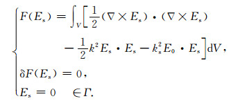
|
(8) |
用有限元直接求解变分问题式(8),可以采用矢量有限元方法,也可以采用节点有限元方法.采用矢量有限元方法(Jin,2002;杨军等,2015)难于模拟电导率连续变化的情况,因此这里采用节点有限元求解式(8).
2.1 网格剖分及插值三维有限元单元类型中,规则六面体单元由于其算法易实现且精度较高而被广泛应用,但对复杂地质体边界的适应性较差, 解决该问题可以在复杂边界处用大量的、细小的单元来实现渐进过渡,但大量的节点和单元增加了有限元计算规模,因此,这里采用任意形状的六面体单元(图 2a)对全区域进行三维不等距网格剖分.为了便于计算,对剖分网格中的任意六面体单元进行等参变换,将直角坐标系(x, y, z)内不规则的六面体单元(图 2a)转换成自然坐标系下的正方形网格(图 2b),这样,式(8)在全区域的积分可分解为各六面体等参单元的积分,有
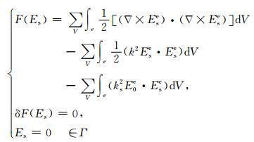
|
(9) |

|
图 2 任意形状的六面体单元示意图 (a)子单元;(b)母单元. Fig. 2 Schematic diagram for an arbitrary hexahedron element (a) Sub-element; (b) Parent element. |
式中,子单元中的体积元dV与母单元中的体积元dζdηdγ的关系为
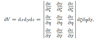
|
(10) |
为了达到模拟任意各向异性电导率连续变化的目的,将任意各向异性电导率赋值于子单元的8个节点而不是赋值于子单元,子单元内的一次电场、二次电场、任意各向异性电导率和任意各向异性异常电导率均呈三线性变化,每个单元内满足如下的表达式:
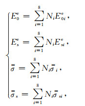
|
(11) |
式中,i=1, 2, 3, 4, 5, 6, 7, 8;E0ie为单元节点i上的一次电场值;Esie为单元上节点i上的待定二次电场值,


|
(12) |
式中,ζi、ηi、γi是自然坐标系(ζ, η, γ)下节点i的坐标.
2.2 单元分析方程(9)中第1式的第一项单元积分:
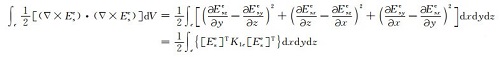
|
(13) |
式中,Ese为单元内的二次电场,

|
方程(9)中第1式的第二项单元积分
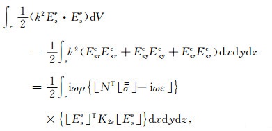
|
(14) |
式中,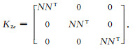
方程(9)中第1式的第三项单元积分
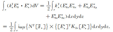
|
(15) |
为了避免伪解的出现,在单元e内将式(13)、式(14)和式(15)中的积分项相加并强加散度条件(Jin,2002),再扩展到总体节点求变分,得到线性方程组
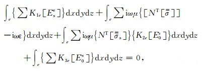
|
(16) |
式中,
|
代入边界条件,采用不完全Cholesky分解-双复共轭梯度法(张永杰和孙秦,2007)求解线性方程组式(16),获得二次电场Es,再加上由解析解计算获得的一次电场E0获得总电场E;利用电场与磁场的关系式(1)获得总磁场E;采用传统定义方法可获得地表测量点Rx卡尼亚视电阻率ρxy、ρyx和相位φxy、φyx,有
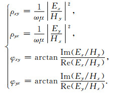
|
(17) |
为了检验本文算法的可靠性和有效性,设计了电导率各向异性且连续变化一维模型以及三维地电模型电导率随位置线性变化且各向同性、主轴各向异性、方位各向异性和倾斜各向异性的情况进行正演计算.在数值模拟计算中,均考虑空气层的影响,设定电导率为1×10-12S·m-1,采用非均匀网格剖分,网格大小为61×61×51.
3.1 电导率各向异性且连续变化一维模型一维模型选用四层理论地电模型M1,其中第二层为电导率垂直各向异性且电导率分层均匀层,第三层为电导率各向异性且连续变化层,其余各层为电导率各向同性且分层均匀层.如图 3所示,第一层电导率为σ1x=σ2x=σ3x=0.01 S·m-1,厚度为h1=500 m;第二层垂直各向异性电导率分别为σ2x=σ2y=0.02 S·m-1,σ2z=1/750 S·m-1,厚度为h2=200 m;第三层电导率垂直各向异性且随着深度z线性变化,垂直各向异性电导率σ3x、σ3y、σ3z从第二层电导率σ2x、σ2y、σ2z线性变化到第四层电导率σ4x、σ4y、σ4z,其中σ3x和σ3y随着深度线性减小而σ3z随着深度线性增加,变化关系如图中所示,D表示第三层任意点的深度,层厚度为h3=200 m;第四层电导率为σ4x=σ4y=σ4z=1/550 S·m-1.发射源Tx是长度为1000 m的接地长导线,其方向平行于x轴且中心坐标为(0, -10000, 0)m;发射电流为30A,发射频率范围为10-4~10-2Hz,共26个频点.

|
图 3 电导率各向异性且连续变化一维模型示意图 Fig. 3 Schematic diagram of 1-D CSAMT model for arbitrary anisotropic and layered homogeneous electrical medium |
图 3所示的理论地电模型未见相应的解析算法,这里,采用渐进过渡的方法将图 3中电导率各向异性且连续变化的第三层分别剖分为1层(如图 4中的M2)、5层(如图 4中的M3)和20层(如图 4中的M4),假定每层的电导率分层均匀,电导率各向异性主轴分量σx、σy和σz随深度z变化如图 4所示,该电导率各向异性且分层均匀层状模型存在解析解.图 3坐标原点处视电阻率ρxy和相位φxy三维有限元计算结果与图 3近似模型(M2、M3和M4三种情况)坐标原点处视电阻率和相位的解析计算结果比较见表 1,相应的视电阻率和相位曲线如图 5所示,M2、M3和M4解析解的计算采用乌普萨拉大学Li和Pedersen开发的开源LANISO程序进行计算(Li and Pedersen, 1991,1992).从图 5可以看出,M2、M3和M4向电导率各向异性且线性变化介质模型逐渐过渡,其解析解的视电阻率和相位曲线与图 3所示模型三维有限元数值解的视电阻率和相位曲线逐渐吻合,由表 1可以看出数值也逐渐接近,表明本文的方法能够有效地模拟电导率各向异性且连续变化三维CSAMT电磁响应.

|
图 4 电导率各向异性且分层均匀一维模型示意图 (a) σx-z变化模型;(b) σy-z变化模型;(c) σz-z变化模型. Fig. 4 Schematic diagram of 1-D CSAMT model for electrical medium with arbitrary anisotropy and layered homogeneous (a) σx changes in the z direction; (b) σy changes in the z direction; (c) σz changes in the z direction. |
|
|
表 1 电导率各向异性且连续变化模型三维有限元数值模拟解与渐进模型解析解计算结果 Table 1 The analytical solutions of the progressive model and the 3-D FEM solutions for electrical medium with arbitrary anisotropy and continuous variation |

|
图 5 电导率各向异性且连续变化一维模型三维有限元计算结果与渐进模型解析解结果对比 (a)视电阻率ρxy;(b)相位φxy. Fig. 5 Comparison between the analytical solutions of the progressive model and the 3-D FEM solutions for electrical medium with arbitrary anisotropy and continuous variation (a) Apparent resistivity ρxy; (b) Phase φxy. |
为了进一步验证本文算法的可靠性和有效性,研究比较电导率连续变化且主轴各向异性、方位各向异性和倾斜各向异性与各向同性情况的差异,设计电导率各向异性且连续变化三维模型,如图 6a所示.均匀半空间存在编号为①、②、③、④和⑤的五个异常体,埋深均为200 m,大小均为600×400×400 m,异常体与异常体、异常体与周围介质的电导率随空间位置呈线性变化(如图 6b和图 6c所示);均匀半空间、异常体①、异常体②、异常体③和异常体④是电导率各向同性介质,且电导率分别为0.01 S·m-1、0.05 S·m-1、0.002 S·m-1、0.05 S·m-1和0.002 S·m-1;异常体⑤电导率分各向同性M5、主轴各向异性M6、水平各向异性M7和倾斜各向异性M8四种情况,其相应电导率张量参数σx、σy、σz、α、β、γ如表 2所示;发射源Tx(长度和电流强度分别为1000 m和30 A)方向平行于y轴且中心坐标为(-10000、0、0)m.图 7是发射源Tx发射频率为10 Hz时地表x=-200 m、x=0 m和x=400 m剖面(y=-2000~2000 m,z=0 m)的视电阻率ρyx和相位φyx曲线,图 8是发射源Tx发射频率为10Hz时的视电阻率等值线和相位等值线.由图 7、图 8可以看出,相对于电导率各向异性M5情况,电导率主轴各向异性M6、电导率方位各向异性M7和电导率倾斜各向异性M8对视电阻率和相位数据影响非常明显,不仅改变数值大小而且改变异常分布,甚至淹没异常体的存在.

|
图 6 电导率各向异性且连续变化三维模型示意图 (a)三维模型示意图;(b)平面图;(c)断面图. Fig. 6 Schematic diagram for the 3D model for electrical medium with arbitrary anisotropy and continuous variation (a) Schematic diagram for the 3D model; (b) Planar view; (c) Section view. |
|
|
表 2 异常体⑤电导率张量的参数值 Table 2 The parameter value of the conductivity tensor of the fifth abnormal body |

|
图 7 不同电导率各向异性类型不同剖面的三维有限元数值模拟结果 (a1,a2) x=-200 m剖面的视电阻率和相位;(b1,b2) x=0 m剖面的视电阻率和相位;(c1,c2) x=400 m剖面的视电阻率和相位. Fig. 7 Numerical simulation results of 3D finite element method of different profiles for different anisotropic conductivity models (a1, a2) Show the apparent resistivity and phase when the section x-axis is a -200 meter; (b1, b2) Show the apparent resistivity and phase when the section x-axis is a 0 meter; (c1, c2) Show the apparent resistivity and phase when the section x-axis is a 400 meter. |

|
图 8 频率为10 Hz时地表视电阻率(Ωm)和相位(°)等值线图 (a1, a2, a3, a4)分别为异常体⑤为电导率各向同性、主轴各向异性、方位各向异性和倾斜各向异性的视电阻率; (b1, b2, b3, b4)分别为异常体⑤为电导率各向同性、主轴各向异性、方位各向异性和倾斜各向异性的相位. Fig. 8 Contour plots of the apparent resistivity and phase on the ground at 10 Hz (a1, a2, a3, a4) are the apparent resistivity when the conductivity of abnormal body ⑤ is isotropic, principal axial anisotropic, azimuthal anisotropic, and oblique anisotropic respectively; (b1, b2, b3, b4) are the apparent phase when the conductivity of abnormal body ⑤ is isotropic, principal axial anisotropic, azimuthal anisotropic, and oblique anisotropic respectively. |
本文提出了一种基于电导率任意各向异性且分块连续变化CSAMT三维有限元数值模拟方法.在数值计算中,采用解析法求解一次场、用有限元求解二次场有效地解决了源点数值的奇异性,一方面提高了数值模拟计算精度,另一方面不需要在源点处增加网格而增加有限元方法的计算工作量;与先求洛伦兹规范下的电磁势再利用差分形式求取电磁场相比,采用直接求解电磁场的有限元法精度更高;采用增加罚项强加散度条件和考虑电导率连续变化,有效解决了节点有限元又可能出现伪解的问题;在网格单元中同时对任意各向异性电导率及二次场进行三线性插值,这个新的数值模拟方法能模拟实际地球介质电导率任意各向异性及随位置连续变化三维CSAMT电磁响应;一维电导率各向异性且连续变化模型激计算结果与电导率渐进模型解析解结果的对比验证了本文基于二次场电导率任意各向异性且分块连续变化CSAMT三维有限元数值模拟方法的有效性;电导率各向异性且连续变化三维地电模型的有限元模拟结果表明,相对于电导率各向异性且连续变化情况,电导率主轴各向异性、方位各向异性和倾斜各向异性对CSAMT视电阻率和相位数据均有明显的影响.
Ansari S, Farquharson C G. 2014. 3D finite-element forward modeling of electromagnetic data using vector and scalar potentials and unstructured grids. Geophysics, 79(4): E149-E165. DOI:10.1190/geo2013-0172.1 |
Avdeev D, Knizhnik S. 2009. 3D integral equation modeling with a linear dependence on dimensions. Geophysics, 74(5): F89-F94. DOI:10.1190/1.3190132 |
Badea E A, Everett M E, Newman G A, et al. 2001. Finite-element analysis of controlled-source electromagnetic induction using Coulomb-gauged potentials. Geophysics, 66(3): 786-799. DOI:10.1190/1.1444968 |
Ben F, Liu Y H, Huang W, et al. 2016. MCSEM Responses for Anisotropic Media in Shallow Water. Journal of Jilin University (Earth Science Edition) (in Chinese), 46(2): 581-593. |
Boerner D E, Wright J A, Thurlow J G, et al. 1993. Tensor CSAMT studies at the Buchans Mine in central Newfoundland. Geophysics, 58(1): 12-19. DOI:10.1190/1.1443342 |
Borner R U. 2010. Numerical modelling in geo-electromagnetics: Advances and challenges. Surveys in Geophysics, 31(2): 225-245. DOI:10.1007/s10712-009-9087-x |
Chen G B, Wang H N, Yao J J, et al. 2009. Three-dimensional numerical modeling of marine controlled-source electromagnetic responses in a layered anisotropic seabed using integral equation method. Acta Physica Sinica (in Chinese), 58(6): 3848-3857. |
Fu C M, Di Q Y, An Z G. 2013. Application of the CSAMT method to groundwater exploration in a metropolitan environment. Geophysics, 78(5): B201-B209. DOI:10.1190/geo2012-0533.1 |
Grayver A V, Kolev T V. 2015. Large-scale 3D geoelectromagnetic modeling using parallel adaptive high-order finite element method. Geophysics, 80(6): E277-E291. DOI:10.1190/geo2015-0013.1 |
Grayver A V, Bürg M. 2014. Robust and scalable 3-D geo-electromagnetic modelling approach using the finite element method. Geophysical Journal International, 198(1): 110-125. DOI:10.1093/gji/ggu119 |
Herwanger J V, Pain C C, Binley A, et al. 2004. Anisotropic resistivity tomography. Geophysical Journal International, 158(2): 409-425. DOI:10.1111/j.1365-246X.2004.02314.x |
Hou J S, Mallan R K, Torres-Verdín C. 2006. Finite-difference simulation of borehole EM measurements in 3D anisotropic media using coupled scalar-vector potentials. Geophysics, 71(5): G225-G233. DOI:10.1190/1.2245467 |
Hu X Y, Peng R H, Wu G J, et al. 2013. Mineral Exploration using CSAMT data: Application to Longmen region metallogenic belt, Guangdong Province, China. Geophysics, 78(3): B111-B119. DOI:10.1190/geo2012-0115.1 |
Jahandari H, Farquharson C G. 2014. A finite-volume solution to the geophysical electromagnetic forward problem using unstructured grids. Geophysics, 79(6): E287-E302. DOI:10.1190/geo2013-0312.1 |
Jin J M. 2002. The Finite Element Method in Electromagnetics. 2nd ed. New York: Wiley-IEEE Press.
|
Key K. 2009. 1D inversion of multicomponent, multifrequency marine CSEM data: methodology and synthetic studies for resolving thin resistive layers. Geophysics, 74(2): F9-F20. DOI:10.1190/1.3058434 |
Kong F N, Johnstad S E, Røsten T, et al. 2008. A 2.5D finite-element-modeling difference method for marine CSEM modeling in stratified anisotropic media. Geophysics, 73(1): F9-F19. DOI:10.1190/1.2819691 |
Li J H, Farquharson C G, Hu X Y. 2016. A vector finite element solver of three-dimensional modelling for a long grounded wire source based on total electric field. Chinese Journal of Geophysics (in Chinese), 59(4): 1521-1534. DOI:10.6038/cjg20160432 |
Li X B, Pedersen L B. 1991. The electromagnetic response of an azimuthally anisotropic half-space. Geophysics, 56(9): 1462-1473. DOI:10.1190/1.1443166 |
Li X B, Pedersen L B. 1992. Controlled-source tensor magnetotelluric responses of a layered earth with azimuthal anisotropy. Geophysical Journal International, 111(1): 91-103. DOI:10.1111/j.1365-246X.1992.tb00557.x |
Li Y, Lin P R, Liu W Q, et al. 2017. 2.5-D numerical simulation of the marine controlled-source electromagnetic method based on isoparametric FEM for the conductivity orthotropic medium. Chinese Journal of Geophysics (in Chinese), 60(2): 748-765. DOI:10.6038/cjg20170226 |
Li Y G, Dai S K. 2011. Finite element modelling of marine controlled-source electromagnetic responses in two-dimensional dipping anisotropic conductivity structures. Geophysical Journal International, 185(2): 622-636. DOI:10.1111/j.1365-246X.2011.04974.x |
Li Y G, Luo M, Pei J X. 2013. Adaptive finite element modeling of marine controlled-source electromagnetic fields in two-dimensional general anisotropic media. Journal of Ocean University of China, 12(1): 1-5. DOI:10.1007/s11802-013-2110-3 |
Linde N, Pedersen L B. 2004. Evidence of electrical anisotropy in limestone formations using the RMT technique. Geophysics, 69(4): 909-916. DOI:10.1190/1.1778234 |
Løseth L O, Ursin B. 2007. Electromagnetic fields in planarly layered anisotropic media. Geophysical Journal International, 170(1): 44-80. DOI:10.1111/j.1365-246X.2007.03390.x |
Negi J G, Saraf P D. 1992. Anisotropy in Geoelectromagnetism (in Chinese). Zou Y H, Chen D Z, trans. Beijing: Geological Publishing House.
|
Newman G A, Commer M, Carazzone J J. 2010. Imaging CSEM data in the presence of electrical anisotropy. Geophysics, 75(2): F51-F61. DOI:10.1190/1.3295883 |
Puzyrev V, Koldan J, De La Puente J, et al. 2013. A parallel finite-element method for three-dimensional controlled-source electromagnetic forward modelling. Geophysical Journal International, 193(2): 678-693. DOI:10.1093/gji/ggt027 |
Ruan B Y, Xu S Z. 1998. FEM for modeling resistivity sounding on 2-D geoelectric model with line variation of conductivity within each block. Earth Science—Journal of China University of Geosciences (in Chinese), 23(3): 303-307. |
Schwarzbach C, Börner R U, Spitzer K. 2011. Three-dimensional adaptive higher order finite element simulation for geo-electromagnetics—a marine CSEM example. Geophysical Journal International, 187(1): 63-74. DOI:10.1111/j.1365-246X.2011.05127.x |
Streich R, Becken M. 2011. Sensitivity of controlled-source electromagnetic fields in planarly layered media. Geophysical Journal International, 187(2): 705-728. DOI:10.1111/j.1365-246X.2011.05203.x |
Tang W W, Liu J X, Tong X Z. 2013. Finite element forward modeling on line source of FCSEM for continuous conductivity. Journal of Jilin University (Earth Science Edition) (in Chinese), 43(5): 1646-1654. |
Tsili W, Fang S. 2001. 3-D electromagnetic anisotropy modeling using finite differences. Geophysics, 66(5): 1386-1398. DOI:10.1190/1.1486779 |
Wang X J, He L F, Chen L, et al. 2017. Mapping deeply buried karst cavities using controlled-source audio magnetotellurics: A case history of a tunnel investigation in southwest China. Geophysics, 82(1): EN1-EN11. DOI:10.1190/geo2015-0534.1 |
Wannamaker P E. 1997. Tensor CSAMT survey over the Sulphur Springs thermal area, Valles Caldera, New Mexico, United States of America, Part Ⅰ: Implications for structure of the western caldera. Geophysics, 62(2): 451-465. DOI:10.1190/1.1444156 |
Yang J, Liu Y, Wu X P. 2015. 3D simulation of marine CSEM using vector finite element method on unstructured grids. Chinese Journal of Geophysics (in Chinese), 58(8): 2827-2838. DOI:10.6038/cjg20150817 |
Yin C C. 1997. Electromagnetic Induction in A Layered Conductor with Arbitrary Anisotropy. Aufl-Göttingen: Cuvillier Verlag.
|
Yin C C, Ben F, Liu Y H, et al. 2014. MCSEM 3D modeling for arbitrarily anisotropic media. Chinese Journal of Geophysics (in Chinese), 57(12): 4110-4122. DOI:10.6038/cjg20141222 |
Zhang Y J, Sun Q. 2007. Preconditioned bi-conjugate gradient method of large-scale complex linear equations. Computer Engineering and Applications (in Chinese), 43(36): 19-20. |
Zhou J M, Zhang Y, Wang H N, et al. 2014. Efficient simulation of three-dimensional marine controlled-source electromagnetic response in anisotropic formation by means of coupled potential finite volume method. Acta Physica Sinica (in Chinese), 63(15): 159101. |
Negi J G, Saraf P D. 1992.大地介质电磁各向异性问题.邹永辉, 陈德志译.北京: 地质出版社.
|
贲放, 刘云鹤, 黄威, 等. 2016. 各向异性介质中的浅海海洋可控源电磁响应特征. 吉林大学学报(地球科学版), 46(2): 581-593. |
陈桂波, 汪宏年, 姚敬金, 等. 2009. 各向异性海底地层海洋可控源电磁响应三维积分方程法数值模拟. 物理学报, 58(6): 3848-3857. DOI:10.3321/j.issn:1000-3290.2009.06.039 |
李建慧, Farquharson C G, 胡祥云, 等. 2016. 基于电场总场矢量有限元法的接地长导线源三维正演. 地球物理学报, 59(4): 1521-1534. DOI:10.6038/cjg20160432 |
李勇, 林品荣, 刘卫强, 等. 2017. 2.5维电导率正交各向异性海洋可控源电磁等参有限元数值模拟. 地球物理学报, 60(2): 748-765. DOI:10.6038/cjg20170226 |
阮百尧, 徐世浙. 1998. 电导率分块线性变化二维地电断面电阻率测深有限元数值模拟. 地球科学—中国地质大学学报, 23(3): 303-307. |
汤文武, 柳建新, 童孝忠. 2013. 电导率连续变化的线源FCSEM有限元正演模拟. 吉林大学学报(地球科学版), 43(5): 1646-1654. |
杨军, 刘颖, 吴小平. 2015. 海洋可控源电磁三维非结构矢量有限元数值模拟. 地球物理学报, 58(8): 2827-2838. DOI:10.6038/cjg20150817 |
殷长春, 贲放, 刘云鹤, 等. 2014. 三维任意各向异性介质中海洋可控源电磁法正演研究. 地球物理学报, 57(12): 4110-4122. DOI:10.6038/cjg20141222 |
张永杰, 孙秦. 2007. 大型复线性方程组预处理双共轭梯度法. 计算工程与应用, 43(36): 19-20. |
周建美, 张烨, 汪宏年, 等. 2014. 耦合势有限体积法高效模拟各向异性地层中海洋可控源的三维电磁响应. 物理学报, 63(15): 159101. DOI:10.7498/aps.63.159101 |