 2019, Vol. 62


2. 安徽省地质调查院(安徽省地质科学研究所), 合肥 230001;
3. 有色金属成矿预测与地质环境监测教育部重点实验室, 长沙 410083
2. Geological Survey of Anhui Province(Anhui Institute of Geological Sciences), Hefei 230001, China;
3. Key Laboratory of Metallogenic Prediction of Non-ferrous Metals and Geological Environment Monitoring, Ministry of Education, Changsha 410083, China
大地电磁法以天然平面电磁波为场源,通过在地表观测相互正交的电磁场分量来获取地下的电性结构信息(Tikhonov, 1950; Cagniard, 1953;汤井田等2017, 2018),是目前研究岩石圈及上地幔电性结构及构造特征的一种重要方法(魏文博等, 2006; Candansayar and Tezkan, 2010; Tang et al., 2013;强建科等, 2014; Li G et al., 2017; Hu et al., 2018; Mo et al., 2017; Li J et al., 2019).由于地球构造应力场、地球形变带、岩石裂隙、空隙水及地质沉积等因素的综合影响,造成地球电导率的分布呈各向异性现象.而基于各向同性假设的模型,无法合理解释含各向异性介质的大地电磁勘探数据(Li, 2002;Wannamaker, 2005).随着计算机技术和各向异性理论的发展,大地电磁各向异性数值模拟已成为研究的前沿(Li and Pek, 2008; Qin et al., 2013a, b ;霍光谱等, 2015;嵇艳鞠等,2016;邱长凯等,2018).
对于简单的二维各向异性地电模型,电磁响应存在解析计算表达式(Qin et al., 2013a, b );而对于复杂的各向异性地电模型,须借助高精度的数值模拟方法来求解.目前,常用于各向异性电磁法数值模拟的方法有:积分方程法、有限差分法和有限单元法.积分方程法具有半解析解的精度,只需要对异常体进行网格剖分,具有未知数少的特点,但存在求解耗时和不适合处理带地形问题等缺陷(陈桂波等, 2009, 2010; Sun, 2015;任政勇等, 2017);有限差分法具有简单的数学表达形式,且生成的是定带宽线性方程组,便于求解,但是该方法不适合模拟带地形的复杂模型(Saraf et al., 1986; Pek and Verner, 1997;霍光谱等, 2015);有限单元法可以采用非结构化网格,适合模拟带任意地形的复杂模型(Reddy and Rankin, 1975; Li, 2002; Li and Pek, 2008; Ren et al., 2013; Fu and Gao, 2017).
有限体积法是基于有限差分和有限元两种方法发展而来的一种数值模拟方法,它兼顾有限差分法和有限元法的优点:1)线性方程组表达形式简单;2)能够采用非结构化网格剖分,适合处理带任意地形的复杂模型(Caughey and Jameson, 1981; Trompert and Hansen, 1996;谢德馨和杨仕友, 2009; Du et al., 2016).近几年来,该方法在地球物理勘探中的应用逐渐发展起来.众多学者采用基于正交网格的有限体积法,研究了电磁法的正演模拟问题(周建美等, 2014;彭荣华等, 2016),但由于这种网格本身的缺陷,对于带地形的复杂模型难以进行精确的模拟.而基于非结构化网格的有限体积法,虽然能够很好的处理带任意地形的复杂模型(Jahandari and Farquharson, 2014, 2015; Du et al., 2016),但是对于带任意地形的复杂各向异性模型的电磁响应,利用有限体积法仍未得到有效的模拟.
为了解决复杂地形情况下二维各向异性大地电磁正演问题,本文开发了基于非结构化三角形网格的有限体积正演算法.并采用本文算法、解析算法、有限元算法分别对层状各向异性模型和复杂各向异性模型进行计算,结果表明本文算法能够稳定、可靠地求解带任意地形的复杂电导率各向异性模型的大地电磁响应.
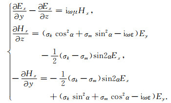
1 正演理论 1.1 边值问题大地电磁场满足如下麦克斯韦方程(取时间因子e-iωt):

|
(1) |
|
(2) |
式中E和H分别为电场和磁场,ε为介电常数,ω=2πf为角频率,f为频率,
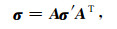
如图 1所示,假设电性主轴i与直角坐标系x方向(构造走向)一致,考虑电性主轴k, m分别与y, z坐标轴成一角度α(徐世浙和赵生凯, 1985; Li, 2002).在直角坐标系中,电导率张量σ可表示为:
|
(3) |

|
图 1 二维各向异性电导率示意图 Fig. 1 Illustration of 2D anisotropic conductivity model |
式中A为坐标变换张量:

|
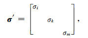
σ′为对角矩阵:
|
其中,σi、σk和σm分别为电性主轴i、k和m方向上的电导率.
对于二维介质,电磁场沿构造走向x方向保持不变(即
TE极化:
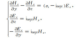
|
(4) |
TM极化:
|
(5) |
方程组(4)和方程组(5)可以写成统一的表达形式:

|
(6) |
式中,∇为梯度算子.对于TE极化模式,u=Ex,


|
有限体积法存在两种方式:单元中心方式和节点中心方式(Caughey and Jameson, 1981;谢德馨和杨仕友, 2009).单元中心方式将单一的网格单元作为控制体单元,并假设单元内电磁场为常数,该方式存在难以求解辅助电磁场的缺陷(Trompert and Hansen, 1996; Du et al., 2016).而节点中心方式以网格节点为中心形成控制体单元,并将未知场置于节点处,借助于线性形函数,可以容易地计算辅助电磁场.因此,本文采用节点中心方式的有限体积法进行模拟.
为了处理任意地形和复杂电导率结构模型,本文采用开源剖分程序Triangle(Shewchuk, 1996)对求解区域Ω进行三角单元网格剖分.在Ω上选取任意节点vi(如图 2所示),依次相连以vi为顶点的三角单元的形心和三角单元各边的中点,形成一个封闭多边形ci,称为包含节点vi的控制体单元.

|
图 2 vi节点的控制体单元ci(Pt是控制单元与第t个三角形的公共部分) Fig. 2 A sketch of the node-centered volume ci which is supported by vi (Pt is a shared polygon by the t-th triangle and the control volume ci) |
方程(6)在控制体单元ci上的积分可以表示为:
|
(7) |
利用散度定理(Jin, 2002),方程(7)可化为如下积分:
|
(8) |
其中,

|
(9) |
将(9)式代入方程(8)可得:
|
(10) |
(10) 式写成矩阵的形式是:

|
(11) |
其中,U为Nn个节点上的未知场向量,A为大型稀疏系数矩阵,其系数表达式为:

|
(12) |
其中,i, k=1, 2, …, Nn.
事实上,控制体单元ci是由一系列多边形Pt(t=1, 2, …, np,np是以节点vi为顶点的三角形的总数)组成.因此,A矩阵的系数又可写为:

|
(13) |
其中,
求解方程(11)中的U需要添加适当的边界条件.当电导率各向异性异常体距离截断边界

|
(14) |

|
(15) |
从而计算出视电阻率和相位值:
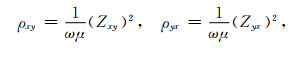
|
(16) |

|
(17) |
其中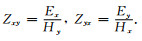
首先,采用具有解析解的层状各向异性模型来验证本文算法的正确性.模型参数如图 3所示,其中第一层和背景层均为各向同性层,电阻率分别为ρ1=10 Ωm和ρ3=1000 Ωm,第二层为ρ2i=200 Ωm,ρ2k=2 Ωm,ρ2m=40 Ωm,α2=60°,h2=4 km的各向异性层,顶部埋深1 km.采用三角形单元进行网格剖分(如图 4),单元个数为550338,节点个数为275408,22个计算频点按对数均匀分布在10-5~102Hz.如图 5所示,将本文计算结果与解析解(Li, 2002)进行对比,可以看出两者的计算结果十分吻合,视电阻率相对误差小于1.3%,相位残差小于0.3°,证明了本文算法的正确性.

|
图 3 含有各向异性层的三层模型 Fig. 3 Three-layer model with an anisotropic layer |

|
图 4 三层层状模型的非结构化网格图 Fig. 4 The triangulation grids for three-layer model |

|
图 5 三层各向异性模型视电阻率及相位值 (a)视电阻率值; (b)相位值; (c)视电阻率相对误差; (d)相位残差. Fig. 5 The apparent resistivity and phases for three-layer model Panel (a) is for the apparent resistivity value, panel (b) is for the phases, panel (c) shows the relative error of apparent resistivity and panel (d) is for the phase residuals. |
为了进一步验证有限体积法求解大地电磁各向异性问题的能力,选取较为复杂的二维各向异性异常体模型进行计算,将有限体积法的结果与已发表的有限单元法的结果(Li, 2002; Ren, 2014)进行对比.模型参数如图 6所示,背景是ρ1=1000 Ωm的各向同性均匀半空间,各向异性矩形棱柱体电阻率为ρ2i=500 Ωm,ρ2k=10 Ωm,ρ2m=500 Ωm(其中电性主轴i与走向x轴平行),α2=60°.柱体截面宽为2 km,厚为8 km,顶部埋深1 km,沿x轴方向无限延伸.模型计算区域为y∈[-500 km, 500 km],z∈[-500 km, 500 km],计算频率是0.1 Hz,41个测点均匀分布在地表y∈[-4 km, 4 km]上.

|
图 6 二维电导率各向异性模型 Fig. 6 2D anisotropic conductivity model |
采用相同的网格剖分单元(如图 7所示),图 8对比了本文计算结果、Li(2002)的有限元法结果与Ren(2014)的有限元法结果.从图中可以看出,三者的计算结果十分吻合,本文计算的视电阻率与Li的相对误差小于1.5%,与Ren的相对误差小于0.01%.图 9对比了YA=0 km、YB=0.8 km、YC=-0.8 km处三种算法在整个计算频域中的结果,从图中可以看出,有限体积法的计算结果与Li的相对误差均小于1.4%,与Ren的相对误差小于0.38%.该测试结果进一步验证了本文算法的稳定性及准确性.

|
图 7 二维电导率各向异性模型的非结构化网格图 Fig. 7 The triangulation grids for 2D anisotropic conductivity model |

|
图 8 二维各向异性体模型上频率为0.1 Hz时不同方法的视电阻率对比 (a) TE模式视电阻率; (b) TM模式视电阻率; (c)视电阻率相对误差(与Li,2002); (d)视电阻率相对误差(与Ren,2014). Fig. 8 The comparison of the computed apparent resistivity (TE for a, TM for b) and relative error of apparent resistivity (Li (2002) for c, Ren (2014) for d) among our finite-volume solutions and the two finite-element method solutions when f=0.1 Hz |

|
图 9 二维电导率各向异性模型上不同方法的视电阻率对比 (a)A=0处TE、TM模式视电阻率; (b) B=0.8 km、C=0.8 km处TM模式视电阻率; (c)视电阻率相对误差(与Ren,2014); (d)视电阻率相对误差(与Li,2002). Fig. 9 The comparison of the computed apparent resistivity (TE and TM at A=0 for a, TM at B=0.8 km, C=0.8 km for b) and relative error of apparent resistivity (Ren (2014) for c, Li (2002) for d) among our finite-volume solutions and the two finite-element method solutions |
表 1为有限体积法和有限单元法(Ren, 2014)的计算参数.从表中可以看出,在相同的计算平台和网格条件下,对于二维大地电磁各向异性模型的正演,有限体积法与有限单元法的消耗相当.
|
|
表 1 有限体积(FVM)和有限元方法(FEM, Ren, 2014)的计算参数,测试平台为Intel i5-4590 CPU3.5 GHz,8 GB RAM Table 1 Mesh and running parameters for the finite-element solution (Ren, 2014) and our finite-volume solution, the platform is Intel i5-4590 CPU3.5 GHz, 8 GB RAM |
选用背斜山谷模型进一步测试本文算法处理复杂模型的能力.背斜顶部山谷宽为4 km,谷底深为0.5 km,背景电阻率为ρ1=100 Ωm的各向同性结构,各向异性背斜的电阻率为ρ2i=10 Ωm,ρ2k=100 Ωm,ρ2m=500 Ωm,夹角α2=30°,如图 10所示.计算区域为y∈[-1000 km, 1000 km],z∈[-1000 km, 1000 km].19个计算频率按对数均匀分布于10-3~103 Hz,测点位于地表.

|
图 10 背斜山谷模型 Fig. 10 The anticline model with topography |
采用相同的网格剖分单元(如图 11所示),分别使用有限体积法和有限元法(Ren, 2014)计算了该模型的大地电磁响应,图 12为有限体积法计算的结果,图 13是两种方法计算结果的相对误差.从图中可以看出,二者的计算结果非常吻合.TE模型的视电阻率相对误差小于0.95%,相位残差小于0.22°;TM模型的视电阻率相对误差小于0.52%,相位残差小于0.075°.表明本文开发的有限体积算法,能够高精度的模拟带地形的复杂各向异性模型.

|
图 11 背斜山谷模型的非结构化网格图 Fig. 11 The triangulation grids for the anticline model |

|
图 12 背斜山谷模型上有限体积法视电阻率和相位拟断面图 (a) TE模式视电阻率; (b) TM模式视电阻率; (c) TE模式相位; (d) TM模式相位. Fig. 12 The pseudo-sections of apparent resistivity and phases computed by the finite-volume method Panel (a) is for the apparent resistivity in TE model, panel (b) is for the apparent resistivity in TM model, panel (c) is for the phase in TE model and panel (d) is for the phase in TM model. |

|
图 13 背斜山谷模型上,有限体积法和有限单元法计算结果的相对误差分布 (a) TE模式视电阻率相对误差; (b) TM模式视电阻率相对误差; (c) TE模式相位残差; (d) TM模式相位残差. Fig. 13 The pseudo-sections of error computed by the finite-element method and finite-volume method for the anticline model (a) The relative error of apparent resistivity in TE model; (b) The relative error of apparent resistivity in TM model; (c) The residual of phase in TE model and (d) the residual of phase in TM model. |
由图 12可知,TE模式视电阻率和相位拟断面图清楚地显示了背斜的位置和形态.但TM模式中,由于各向异性的影响,视电阻率和相位在背斜核部发生严重畸变,使得TM模式的视电阻率和相位拟断面图无法显示背斜的形态.
3 结论本文开发了一种新的二维大地电磁正演模拟算法.从麦克斯韦方程出发,推导了大地电磁场各向异性介质的边值问题,在控制体单元上,基于散度定理,采用线性插值函数,建立了节点型有限体积法的计算流程,得到电磁场的响应值.通过三种不同复杂度的模型算例对比,得到以下结论:
(1) 本文提出的基于非结构化网格的大地电磁各向异性有限体积算法,是一种能够适合模拟带任意复杂地形模型的高精度、稳定的算法.
(2) 有限体积法基本思路易于理解,基于守恒原理,利用散度定理可直接将复杂的赫姆霍斯方程转换成线性方程组进行求解,原理简单,易于编程实现.
(3) 对于同一模型,在相同的计算平台和网格条件下,有限体积法与广泛应用的有限单元法的计算精度相似,且消耗相当.因此,有限体积法是处理电磁法各向异性问题的另一种有效方法.
致谢感谢Shewchuk提供的非结构三角形网格剖分开源代码Triangle,感谢Schenk提供的方程组求解器Pardiso,感谢网格剖分可视化软件PARAVIEW的作者.
附录A
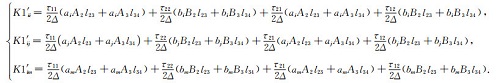
首先考虑式(13)中的第一部分线积分.对于TE模式,
|
(A1) |
其中,


|
附图A1 多边形Pt(i)示意图 Appendix Fig. A1 Illustration of the polygon Pt(i) |
令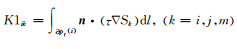

|
(A2) |
其中:
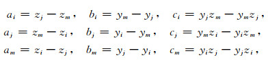
|
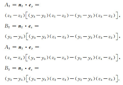
|

对于TM模式,
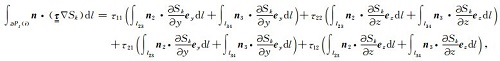
|
(A3) |
其具体表达式为:
|
(A4) |
然后,计算式(13)中的第二部分在多边形pt(i)上的面积分.建立二维自然坐标系Li, Lj, Lm进行坐标转换(如附图A2):
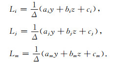
|

|
附图A2 坐标转换图 Appendix Fig. A2 The coordinate transformation |
在多边形pt(i)上1点处:Lj=0, Lm=0;2点处:Lj=1/2, Lm=0;3点处:Lj=1/3, Lm=1/3;4点处:Lj=0, Lm=1/2,所以yz平面上的多边形pt(i)变换成Lj, Lm平面上的四边形.
那么,积分可以表示为:
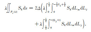
|
(A5) |
令

|
(A6) |
Cagniard L. 1953. Basic theory of the magneto-telluric method of geophysical prospecting. Geophysics, 18(3): 605-635. DOI:10.1190/1.1437915 |
Candansayar M E, Tezkan B. 2010. Two-dimensional joint inversion of radiomagnetotelluric and direct current resistivity data. Geophysical Prospecting, 56(5): 737-749. |
Caughey D A, Jameson A. 1981. Basic advances in the finite-volume method for transonic potential-flow calculations. //Numerical and Physical Aspects of Aerodynamic Flows. Berlin, Heidelberg: Springer, 445-461.
|
Chen G B, Wang H N, Yao J J, et al. 2009. Three-dimensional numerical modeling of marine controlled-source electromagnetic responses in a layered anisotropic seabed using integral equation method. Acta Physica Sinica (in Chinese), 58(6): 3848-3857. |
Chen G B, Wang H N, Yao J J, et al. 2010. Three-dimensional modeling of frequency sounding in layered anisotropic earth using integral equation method. Chinese Journal of Computational Physics (in Chinese), 27(2): 274-280. |
Du H K, Ren Z Y, Tang J T. 2016. A finite-volume approach for 2D magnetotellurics modeling with arbitrary topographies. Studia Geophysica et Geodaetica, 60(2): 332-347. DOI:10.1007/s11200-014-1041-9 |
Fu S B, Gao K. 2017. A fast solver for the Helmholtz equation based on the generalized multiscale finite-element method. Geophysical Journal International, 211(2): 797-813. DOI:10.1093/gji/ggx343 |
Hu S G, Tang J T, Ren Z Y, et al. 2018. Multiple underwater objects localization with magnetic gradiometry. IEEE Geoscience and Remote Sensing Letters, 16(2): 296-300. |
Huo G P, Hu X Y, Huang Y F, et al. 2015. Mt modeling for two-dimensional anisotropic conductivity structure with topography and examples of comparative analyses. Chinese Journal of Geophysics (in Chinese), 58(12): 4696-4708. DOI:10.6038/cjg20151230 |
Jahandari H, Farquharson C G. 2014. A finite-volume solution to the geophysical electromagnetic forward problem using unstructured grids. Geophysics, 79(6): 653-657. |
Jahandari H, Farquharson G C. 2015. Finite-volume modelling of geophysical electromagnetic data on unstructured grids using potentials. Geophysical Journal International, 202(3): 1859-1876. DOI:10.1093/gji/ggv257 |
Ji Y J, Huang T Z, Huang W Y, et al. 2016. 2D anisotropic magnetotelluric numerical simulation using meshfree method under undulating terrain. Chinese Journal of Geophysics (in Chinese), 59(12): 4483-4493. DOI:10.6038/cjg20161211 |
Jin J M. 2002. The Finite Element Method in Electromagnetics. 2nd ed. New York, NY: John Wiley & Sons.
|
Li G, Xiao X, Tang J T, et al. 2017. Near-source noise suppression of AMT by compressive sensing and mathematical morphology filtering. Applied Geophysics, 14(4): 581-589. DOI:10.1007/s11770-017-0645-6 |
Li J, Zhang X, Tang J T, et al. 2019. Audio magnetotelluric signal-noise identification and separation based on multifractal spectrum and matching pursuit. Fractals, 27(1): 1940007. DOI:10.1142/S0218348X19400073 |
Li Y. 2000. Finite element modeling of electromagnetic fields in two-and three-dimensional anisotropic conductivity structures [Ph. D. thesis]. Göttingen: University of Göttingen.
|
Li Y G. 2002. A finite-element algorithm for electromagnetic induction in two-dimensional anisotropic conductivity structures. Geophysical Journal International, 148(3): 389-401. DOI:10.1046/j.1365-246x.2002.01570.x |
Li Y G, Pek J. 2008. Adaptive finite element modelling of two-dimensional magnetotelluric fields in general anisotropic media. Geophysical Journal International, 175(3): 942-954. DOI:10.1111/j.1365-246X.2008.03955.x |
Mo D, Jiang Q Y, Li D Q, et al. 2017. Controlled-source electromagnetic data processing based on gray system theory and robust estimation. Applied Geophysics, 14(4): 570-580. DOI:10.1007/s11770-017-0646-5 |
Pek J, Verner T. 2007. Finite-difference modelling of magnetotelluric fields in two-dimensional anisotropic media. Geophysical Journal International, 128(3): 505-521. |
Peng R H, Hu X Y, Han B, et al. 2016. 3D frequency-domain CSEM forward modeling based on the mimetic finite-volume method. Chinese Journal of Geophysics (in Chinese), 59(10): 3927-3939. DOI:10.6038/cjg20161036 |
Qiang J K, Wang X Y, Tang J T, et al. 2014. The geological structures along Huainan-Liyang magnetotelluric profile: constraints from MT data. Acta Petrologica Sinica (in Chinese), 30(4): 957-965. |
Qin L J, Yang C F, Chen K. 2013a. Quasi-analytic solution of 2-D magnetotelluric fields on an axially anisotropic infinite fault. Geophysical Journal International, 192(1): 67-74. DOI:10.1093/gji/ggs018 |
Qin L J, Yang C F, Chen K. 2013b. Analytic solution to the magnetotelluric response over anisotropic medium and its discussion. Science China Earth Sciences, 56(9): 1607-1615. DOI:10.1007/s11430-013-4585-6 |
Qiu C K, Yin C C, Liu Y H, et al. 2018. 3D forward modeling of controlled-source audio-frequency magnetotellurics in arbitrarily anisotropic media. Chinese Journal of Geophysics (in Chinese), 61(8): 3488-3498. DOI:10.6038/cjg2018L0326 |
Reddy I K, Rankin D. 1975. Magnetotelluric response of laterally inhomogeneous and anisotropic media. Geophysics, 40(6): 1035-1045. DOI:10.1190/1.1440579 |
Ren Z Y, Kalscheuer T, Greenhalgh S, et al. 2013. A goal-oriented adaptive finite-element approach for plane wave 3-D electromagnetic modelling. Geophysical Journal International, 194(2): 700-718. DOI:10.1093/gji/ggt154 |
Ren Z Y. 2014. A C++ based 2D magnetotellurics and radio-magnetotellurics finite element solver using unstructured grids. http://www.complete-mt-solutions.com/mtnet/main/.
|
Ren Z Y, Chen C J, Tang J T, et al. 2017. A new integral equation approach for 3D magnetotelluric modeling. Chinese Journal of Geophysics (in Chinese), 60(11): 4505-4515. |
Saraf P D, Negi J G, erv V. 1986. Magnetotelluric response of a laterally inhomogeneous anisotropic inclusion. Physics of the Earth and Planetary Interiors, 43(3): 196-198. DOI:10.1016/0031-9201(86)90046-4 |
Shewchuk J R. 1996. Triangle: Engineering a 2D quality mesh generator and Delaunay triangulator. //Workshop on Applied Computational Geometry. Berlin, Heidelberg: Springer-Verlag, 203-222.
|
Sun L E. 2015. Electromagnetic modeling of inhomogeneous and anisotropic structures by volume integral equation methods. Waves in Random and Complex Media, 25(4): 536-548. DOI:10.1080/17455030.2015.1058541 |
Tang J T, Zhou C, Wang X Y, et al. 2013. Deep electrical structure and geological significance of Tongling ore district. Tectonophysics, 606: 78-96. DOI:10.1016/j.tecto.2013.05.039 |
Tang J T, Li G, Xiao X, et al. 2017. Strong noise separation for magnetotelluric data based on a signal reconstruction algorithm of compressive sensing. Chinese Journal of Geophysics (in Chinese), 60(9): 3642-3654. DOI:10.6038/cjg20170928 |
Tang J T, Li G, Zhou C, et al. 2018. Denoising AMT data based on dictionary learning. Chinese Journal of Geophysics (in Chinese), 61(9): 3835-3850. DOI:10.6038/cjg2018L0376 |
Tikhonov A N. 1950. On determining electrical characteristics of the deep layers of the earth′s crust. Dolk Acad Nauk SSSR, 73(2): 295-297. |
Trompert R A, Hansen U. 1996. The application of a finite volume multigrid method to three-dimensional flow problems in a highly viscous fluid with a variable viscosity. Geophysical and Astrophysical Fluid Dynamics, 83(3): 261-291. |
Wannamaker P E. 2005. Anisotropy versus heterogeneity in continental solid earth electromagnetic studies: fundamental response characteristics and implications for physicochemical state. Surveys in Geophysics, 26(6): 733-765. DOI:10.1007/s10712-005-1832-1 |
Wei W B, Jin S, Ye G F, et al. 2006. Conductivity structure of crust and upper mantle beneath the northern Tibetan Plateau: Results of super-wide band magnetotelluric sounding. Chinese Journal of Geophysics (in Chinese), 49(4): 1215-1225. |
Xie D X, Yang S Y. 2009. Engineering Electromagnetic Field Numerical Analysis and Synthesis (in Chinese). Beijing: China Machine Press.
|
Xu S Z, Zhao S K. 1985. Solution of magnetotelluric field equations for a two-dimensional, anisotropic geoelectric section by the finite element method. Acta Seismologica Sinica (in Chinese), 7(1): 80-89. |
Zhou J M, Zhang Y, Wang H N, et al. 2014. Efficient simulation of three-dimensional marine controlled-source electromagnetic response in anisotropic formation by means of coupled potential finite volume method. Acta Physica Sinica (in Chinese), 63(15): 159101. |
陈桂波, 汪宏年, 姚敬金, 等. 2009. 各向异性海底地层海洋可控源电磁响应三维积分方程法数值模拟. 物理学报, 58(6): 3848-3857. DOI:10.3321/j.issn:1000-3290.2009.06.039 |
陈桂波, 汪宏年, 姚敬金, 等. 2010. 利用积分方程法的各向异性地层频率测深三维模拟. 计算物理, 27(2): 274-280. DOI:10.3969/j.issn.1001-246X.2010.02.017 |
霍光谱, 胡祥云, 黄一凡, 等. 2015. 带地形的大地电磁各向异性二维模拟及实例对比分析. 地球物理学报, 58(12): 4696-4708. DOI:10.6038/cjg20151230 |
嵇艳鞠, 黄廷哲, 黄婉玉, 等. 2016. 起伏地形下各向异性的2D大地电磁无网格法数值模拟. 地球物理学报, 59(12): 4483-4493. DOI:10.6038/cjg20161211 |
彭荣华, 胡祥云, 韩波, 等. 2016. 基于拟态有限体积法的频率域可控源三维正演计算. 地球物理学报, 59(10): 3927-3939. DOI:10.6038/cjg20161036 |
强建科, 王显莹, 汤井田, 等. 2014. 淮南—溧阳大地电磁剖面与地质结构分析. 岩石学报, 30(4): 957-965. |
邱长凯, 殷长春, 刘云鹤, 等. 2018. 任意各向异性介质中三维可控源音频大地电磁正演模拟. 地球物理学报, 61(8): 3488-3498. DOI:10.6038/cjg2018L0326 |
任政勇, 陈超健, 汤井田, 等. 2017. 一种新的三维大地电磁积分方程正演方法. 地球物理学报, 60(11): 4506-4515. DOI:10.6038/cjg20171134 |
汤井田, 李广, 肖晓, 等. 2017. 基于压缩感知重构算法的大地电磁强干扰分离. 地球物理学报, 60(9): 3642-3654. DOI:10.6038/cjg20170928 |
汤井田, 李广, 周聪, 等. 2018. 基于字典学习的音频大地电磁数据处理. 地球物理学报, 61(9): 3835-3850. DOI:10.6038/cjg2018L0376 |
魏文博, 金胜, 叶高峰, 等. 2006. 藏北高原地壳及上地幔导电性结构——超宽频带大地电磁测深研究结果. 地球物理学报, 49(4): 1215-1225. DOI:10.3321/j.issn:0001-5733.2006.04.038 |
谢德馨, 杨仕友. 2009. 工程电磁场数值分析与综合. 北京: 机械工业出版社: 129-141.
|
徐世浙, 赵生凯. 1985. 二维各向异性地电断面大地电磁场的有限元法解法. 地震学报, 7(1): 80-89. |
周建美, 张烨, 汪宏年, 等. 2014. 耦合势有限体积法高效模拟各向异性地层中海洋可控源的三维电磁响应. 物理学报, 63(15): 159101. DOI:10.7498/aps.63.159101 |