 2019, Vol. 62


欧拉反演方法(Reid et al., 1990)是一种常用的快速确定场源位置的位场反演方法,它是以欧拉齐次方程为基础,运用构造指数、位场异常及其空间导数来圈定场源位置.对于理想模型(如球体、无限长水平圆柱体等),欧拉反演结果是准确的;但是对于稍复杂的地质模型(如长方体、组合场源等),欧拉反演结果是发散的.
为了减小解的发散性并获得稳定的反演结果,前人对欧拉反演方法进行了针对性的研究.研究表明,背景场、噪声、构造指数的选择等是常见的导致反演结果发散的因素(Reid et al., 2014).为了减小背景场对反演结果的影响,提高反演结果的聚集程度,背景场通常被假设为常数(如Thompson, 1982;Nabighian and Hansen, 2001;Gerovska et al., 2005;Davis et al., 2010)、线性函数(Stavrev, 1997)或非线性函数(Dewangan et al., 2007);为了减小噪声等的影响,可以采用向上延拓对磁异常数据进行预处理(如Salem et al., 2007;Florio et al., 2014).姚长利等(2004)只对水平梯度较大的区域内的反演结果进行筛选和结果统计评价,有效地减小了解的发散性,加快了欧拉反演的实用化进程;为了减小构造指数对反演结果的影响,部分研究人员(如Barbosa et al., 1999;Martelet et al., 2001;Stavrev and Reid, 2006;Reid and Thurston, 2014;Fedi,2016;Melo and Barbosa, 2018)提出了确定构造指数的方法,但是目前还没有一种普遍有效的方法,选择将构造指数当作未知数进行反演还是主要的处理方式.另外,Salem等(2007)将倾斜角与欧拉反演方法相结合,消除了欧拉方程中的构造指数,避免了因构造指数选择不当而造成反演结果的发散.
虽然前人在减小解的发散性方面做了许多研究工作,但是该问题依然没有得到解决.在进行欧拉反演计算时,最小二乘法是求解线性方程组的常用方法(Hansen and Suciu, 2002;Gerovska and Araúzo-Bravo,2003;Melo et al., 2013).但是在求解方程组时,若系数矩阵奇异,最小二乘法将无法获得反演结果.处理奇异矩阵的方法主要包括奇异值分解、阻尼最小二乘法、正则化方法等,可以采用上述方法处理奇异矩阵并进行反演计算.范美宁(2006)为了减少欧拉反演的计算量,对欧拉线性方程组的系数矩阵进行了奇异值分解(SVD),但是并没有明显地减小反演结果的发散性.Beiki(2013)为使不确定性估计量接近于零,将截断奇异值分解应用到欧拉反演方法中,但是也没有明显减小解的发散性.当欧拉线性方程组的系数矩阵奇异时,SVD方法可以获得反演结果.对于非奇异矩阵,SVD和最小二乘方法获得的解是相同的.SVD方法实际上并没有对系数矩阵进行改变,因此在欧拉反演中,相对于最小二乘法,SVD方法也无法明显地减小解的发散性.阻尼最小二乘法、正则化方法等是通过改变系数矩阵来达到减小矩阵奇异程度的方法,其中阻尼最小二乘法是一种较为简单的改变系数矩阵的方法.本文采用阻尼最小二乘法进行反演计算,并且通过对阻尼因子、系数矩阵以及坐标原点位置对阻尼最小二乘法欧拉反演结果的影响进行详细分析,得出该方法的内在规律性,在此基础上实现了减小反演结果的发散性的目的.下面我们将对其原理、技术及应用效果进行分析介绍.
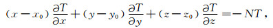
1 方法原理欧拉方程的一般形式(Reid et al., 1990)为
|
(1) |
其中,

|
(2) |
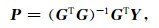
可得到场源参数
|
(3) |
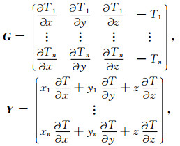
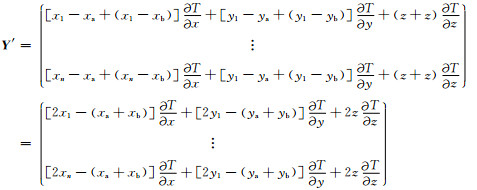
其中P为x0、y0、z0、N,G为n × 4的矩阵,Y为列向量,G、Y的形式如下:
|
(4) |
其中,x1、y1、xn、yn、z为测点坐标.
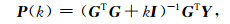
在欧拉反演中,当窗口内的数据具有很高的相似性时,系数矩阵GTG会接近奇异或奇异(Mushayandebvu et al., 2004),此时常规最小二乘法将无法计算反演结果.本文选用阻尼最小二乘法(Marquardt, 1963)进行欧拉反演计算.阻尼最小二乘法是通过对系数矩阵添加偏移对角矩阵D来达到减小矩阵奇异程度的目的.设D=kI,I是单位矩阵,k是大于0的阻尼因子,阻尼最小二乘公式为(Hoerl and Kennard, 1970):
|
(5) |
很明显,GTG+kI奇异的程度要小于GTG.
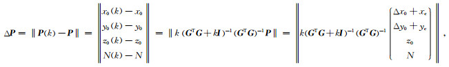
如果方程组的系数矩阵非奇异,P与P(k)存在如下的关系:

|
(6) |
(6) 式表明,对于任意的k>0, ‖P‖≠0总有‖P(k)‖ < ‖P(0)‖(Hoerl and Kennard, 1970),因此相对于P而言,P(k)有向原点压缩的趋势,向原点压缩程度可由公式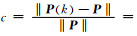
当系数矩阵特征值λ远小于k时,c≈1, P(k)≈0,而当λ远大于k时,c≈0, P(k)≈P.因此特征值不同的系数矩阵对阻尼因子的敏感程度是不同的,λ较小的系数矩阵对阻尼因子更为敏感,对应的反演结果越容易靠近坐标原点,而λ较大的系数矩阵对应的反演结果几乎不受阻尼因子的影响.根据位场理论(以磁为例),通常滑动窗口距离场源越近,系数矩阵的迹越大,对应的特征值也会越大.系数矩阵大小可以根据特征值大小进行定义.图 1是模型算例,用来分析窗口中的系数矩阵λ大小与反演结果向原点压缩程度关系,为简化问题,所选模型为垂直磁化.图 1a是组合场源及选取的滑动窗口示意图,我们选取了数个逐渐远离某场源的滑动窗口进行实验.实验结果表明,随着窗口远离场源,系数矩阵特征值逐渐减小(图 1b),对应的反演结果向原点压缩的程度增大、反演结果越容易靠近坐标原点(图 1c).

|
图 1 系数矩阵大小与反演结果向原点压缩程度分析图 (a)垂直磁化的球体模型,图中的1-6为滑动窗口中心点的位置; (b)滑动窗口中的系数矩阵最大特征值; (c)滑动窗口中的反演结果分布图(图中的数字与a图中的数字对应). Fig. 1 The figures used to analyse the relationship between the normal equations matrix and the accuracy of Euler solutions (a) Synthetic magnetic generated by 7 spheres, vertical magnetization, 1-6 represent the center of the sliding window; (b) The maximum eigenvalues obtained from six windows; (c) The inversion results obtained from the six windows. |
根据图 1和公式(6)可得,阻尼因子会促使远离场源的窗口中产生的反演结果靠近原点,因此当坐标原点位于测区内时,会有大量的虚假反演结果位于测区内(图 2a),而当坐标原点远离场源时,部分反演结果会由于靠近原点而偏离场源,此时测区内反演结果的发散性明显减小(图 2b).因此当坐标原点位于测区内或离测区较近时,我们建议先将坐标原点设置在距离测区较远的位置,然后再进行反演计算.

|
图 2 阻尼最小二乘反演结果随坐标系变化时的分布图 (a)坐标原点位于测区内时的反演结果; (b)坐标原点位于测区外时的反演结果. Fig. 2 The influence of the change of the relative position of the coordinate origin on Euler solutions obtained by damped least square method (DLS) (a) The distribution of the solutions when the coordinate origin is in the study area; (b) The distribution of the solutions when the coordinate origin is out of the study area. |
图 2中,坐标原点相对位置变化后,部分反演结果在测区中的相对位置也随之变化,这是由于阻尼因子会促使部分反演结果向坐标原点方向压缩导致的;而对于常规最小二乘公式而言,反演结果在测区中的相对位置是固定的(图 3a、3b).下面我们将分析坐标原点的相对位置变化对阻尼反演结果的影响.

|
图 3 坐标系变化时的常规最小二乘反演结果分布图 (a)坐标原点位于测区内时的反演结果; (b)坐标原点位于测区以外时的反演结果. Fig. 3 The influence of the change of the relative position of the coordinate origin on Euler solutions obtained by ordinary least square method (OLS) (a) The distribution of the solutions when the coordinate origin is in the study area; (b) The distribution of the solutions when the coordinate origin is out of the study area. |
我们把反演结果距离测区下、左边线的距离记为Δx0, Δy0,测区左下角的坐标记为xc, yc(坐标原点位置变化会影响其数值变化).因此反演结果可写为x0=Δx0+xc, y0=Δy0+yc,根据公式(6),P(k)与P的差为
|
(7) |
(7) 式表明,在某一次数据反演的窗口中,随着坐标原点远离测区,ΔP变大,P(k)偏离P的距离增大,P(k)越容易靠近坐标原点.又由于λ越小,反演结果向原点压缩程度越大.因此随着坐标原点远离测区,远离场源的窗口中产生的反演结果越容易靠近原点而偏离测区,此时测区内虚假反演结果的数量会急剧减少(图 4),反演结果的发散性减小.

|
图 4 坐标原点远离测区时,测区内反演结果的数量变化曲线图 Fig. 4 The number of solutions in study area with the coordinate origin away from the study area |
虽然坐标原点相对位置的变化、系数矩阵等会影响阻尼最小二乘反演结果向原点压缩的程度,但是坐标系尺度的变化并不会影响反演结果向原点压缩的程度(图 5).

|
图 5 变坐标尺度下的反演结果分布情况对比图 (a)微小坐标尺度下的常规最小二乘反演结果;(b)微小坐标尺度下的阻尼最小二乘反演结果;(c)极大坐标尺度下的常规最小二乘反演结果;(d)极大坐标尺度下的阻尼最小二乘反演结果. Fig. 5 The distribution of the inversion results when the coordinate-scale changed (a) The results obtained by OLS when the coordinate-scale is tiny; (b) The inversion results obtained by DLS when the coordinate-scale is tiny; (c) The results obtained by OLS when the coordinate-scale is large; (d) The inversion results obtained by DLS when the coordinate-scale is large. |
综上所述,阻尼最小二乘法可以明显地减小欧拉反演结果的发散性.阻尼最小二乘法实际上是对常规最小二乘法的一种改进,因此它可以应用于任何一种采用最小二乘法进行计算的欧拉反演方法中.
2 解的筛选坐标原点的位置变化会影响部分反演结果在测区中的相对位置,因此可以通过改变坐标原点的相对位置筛选稳定的反演结果.我们把坐标原点分别设置在测区初始坐标系中的(xa, ya)或(xb, yb)处,把某一个滑动窗口在不同坐标系下产生的反演结果相加可得:

|
(8) |
|
其中x1, xn, y1, yn, z为初始坐标系下的测点坐标.公式(8)表明,如果xa+xb=0,ya+yb=0, 那么Pa(k)+Pb(k)=2P(k),其中P(k)是测区初始坐标系下的阻尼最小二乘反演结果.根据上述内容,我们提出了一种新的筛选方法——变坐标系筛选方法.该筛选方法一共分为四步:
第一步:把坐标原点设置在测区左下角(xa, ya),得到一个新测区.在新测区内进行阻尼最小二乘法欧拉反演,保存留在新测区内的反演结果及对应的滑动窗口中心点的相对位置编号(i, j).此时可以认为保存下来的滑动窗口离场源较近.
第二步:把坐标原点设置在测区右上角(-xa, -ya),得到另一个新测区.在测区内进行阻尼最小二乘法欧拉反演,保存留在新测区内的反演结果及对应的滑动窗口中心点的相对位置编号(i, j).
第三步:寻找第一、二步中相同的滑动窗口中心点的位置编号,此时每一个位置编号将会对应两个反演结果(第一、二步各有一个反演结果),然后将这两个反演结果取平均值,得到在原坐标系(i, j)处对应的阻尼最小二乘反演结果.经过前三步筛选后,如果反演结果的发散性仍然较大,可以进行第四步筛选.
第四步:根据移动速率筛选准则(Liu et al., 2019)进行筛选.通常在场源附近,随着滑动窗口的移动,反演结果的变化量是微小的,因此可以根据反演结果的这一特点,对反演结果进行进一步的筛选.移动速率筛选准则是指如果反演结果的移动距离小于n倍(通常n≤1)的滑动窗口的移动距离,则说明反演结果极有可能靠近场源,保存相应的结果.
下面以图 1中的组合模型为例来展示变坐标系筛选方法的筛选过程及效果.首先我们将坐标原点设置在测区的右上角(图 6a)和左下角(图 6c),然后再进行阻尼最小二乘欧拉反演计算.图 6a和6c分别是第一、二步筛选后的反演结果分布图,此时测区内的反演结果的数量及发散性明显较小.图 6e是第三步筛选后的反演结果,此时已经确定了场源水平位置及埋深(未显示).

|
图 6 变坐标系筛选方法确定场源位置的过程及效果图 (a)坐标原点位于测区右上角时反演结果分布图; (b) a图中的反演结果对应的滑动窗口中心点位置; (c)坐标原点位于测区左下角时反演结果分布图; (d) c图中反演结果对应的滑动窗口中心点的位置; (e)将a、c图中相同滑动窗口中的两个反演结果取平均值得到的反演结果分布图; (f) e图中的反演结果对应的滑动窗口中心点位置. Fig. 6 The application of variable coordinate system selection method (a) The Euler solutions obtained by DLS when the origin of the coordinates is in the upper right corner; (b) The position of the sliding window corresponding to the results in (a); (c) The Euler solutions obtained by DLS when the origin of the coordinates is in the lower left corner; (d) The position of the sliding window corresponding to the results in (c); (e) Averaging the inversion results in the same window in (a) and (c); (f) The position of the sliding window corresponding to the results in (e). |
变坐标系筛选方法可以有效地减小组合模型反演结果的发散性(图 6).为了检验我们的筛选方法在确定简单理想场源位置时的筛选效果,我们设计了理想球体模型实验(图 7).对于理想的球体模型,常规欧拉反演方法便可以获得准确的场源位置.当采用阻尼最小二乘法欧拉反演进行反演时,阻尼因子会导致反演结果具有一定的发散性(图 7b、7c).但是通过采用变坐标系筛选方法,我们准确地确定了场源的水平位置及深度(未显示).该实验表明,变坐标系筛选方法可以有效地确定理想场源的位置.

|
图 7 理想模型实验 (a)阻尼最小二乘反演结果分布图; (b)坐标原点位于测区右上角时的反演结果分布图; (c)坐标原点位于测区左下角时的反演结果分布图; (d)变坐标系筛选后的反演结果分布图. Fig. 7 An ideal model test (a) The inversion results generated by DLS; (b) The inversion results when the coordinate origin is in the upper right corner; (c) The inversion results when the coordinate origin is in the lower left corner; (d) The inversion results after selection. |
为了进一步测试阻尼最小二乘法欧拉反演在确定复杂场源位置时的效果,我们将该方法应用于图 8中的复杂模型(Gerovska and Araúzo-Bravo, 2003).该模型由五个简单规则模型组成,模型的具体参数见表 1.模型中S2、S4、S5对应的磁倾角为59°,磁偏角为2.4°,模型S1、S3的磁化方向与S2相反.在这一部分,我们采用Gerovska和Araúzo-Bravo(2003)文章中提到的欧拉算法,滑动窗口尺寸为1.25 km×1.25 km,阻尼因子为2.

|
图 8 磁异常及变坐标系筛选方法确定的反演结果分布图 (a)组合模型磁异常分布图; (b)常规最小二乘反演结果分布图; (c)阻尼最小二乘反演结果分布图; (d)坐标原点位于测区左下角时反演结果分布图;(e)坐标原点位于测区右上角时反演结果分布图; (f)将c、d图中相同滑动窗口中的两个反演结果取平均值后得到的反演结果分布图; (g) d图中的反演结果对应的滑动窗口中心点; (h) e图中的反演结果对应的滑动窗口中心点; (i) f图中的反演结果对应的滑动窗口中心点. Fig. 8 Synthetic data produced by different geometries and the distribution of the Euler solutions (a) Model anomalous magnetic field; (b) The inversion results obtained by OLS; (c) The inversion results obtained by DLS; (d) The distribution of DLS Euler solutions when the coordinate origin is in the lower left corner; (e) The distribution of OLS Euler solutions when the coordinate origin is in the upper right corner; (f) Averaging the Euler solutions in the same sliding window in (c) and (d); (g) The position of the sliding window center corresponding to the results in (d); (h) The position of the sliding window center corresponding to the results in (e); (i) The position of the sliding window center corresponding to the results in (f). |
|
|
表 1 组合模型中各个模型的位置参数 Table 1 The position of the models |
图 8是磁异常等值线图及反演结果分布图.其中图 8b为常规最小二乘欧拉反演结果分布图.图 8e为阻尼最小二乘反演结果分布图.图 8d—e为改变坐标原点位置后的反演结果分布图.由图 8b—e发现,当坐标原点在测区以外时,反演结果的发散性较小.图 8f是经过变坐标系筛选后获得的反演结果(未进行移动速率筛选).为了进一步确定场源位置,我们对反演结果进行了移动速率筛选.筛选完后,在空间某一位置处会有许多反演结果聚集成簇.我们对每一个簇中的数值取平均值,然后将此平均值作为最终的反演结果.图 9是经过移动速率筛选后的反演结果与文献(Gerovska and Araúzo-Bravo, 2003)中的反演结果对比图.图 9a为筛选出的场源位置,该图表明,经过移动速率筛选后确定的场源水平位置与真实场源的水平位置是一致的.图 9b、9d是经过移动速率筛选后的X-Z和Y-Z方向反演结果分布图,图 9c、9e是文献中筛选后的反演结果分布图.对比图 9b—e可以发现,我们筛选出的结果与文献中的结果以及真实场源位置较为接近.但是图 9b—e中筛选出的部分深度值与真实深度值存在一定偏差(如图 9a中的角点1-4),这是由于场源之间的干扰导致的.通过本次模型实验可以发现,变坐标系筛选方法能够较好地筛选出复杂场源的位置.

|
图 9 估算的场源位置分布图 (a)移动速率筛选后的反演结果水平分布图;(b) X-Z方向的反演结果分布图,红色方框为真实场源位置;(c)文献(Gerovska and Araúzo-Bravo, 2003)中的X-Z方向反演结果分布图,红色方框为真实场源位置;(d) Y-Z方向的反演结果分布图; (e)文献(Gerovska and Araúzo-Bravo, 2003)中的Y-Z方向反演结果分布图. Fig. 9 The distribution of the estimated depths (a) The estimated horizontal location of the source after selecting by moving-rate selection method; (b) The projection of the Euler solutions on X-Z plane by our method, the red rectangles respresent the position of the source; (c) The projection of the Euler solutions on X-Z plane by Gerovska and Araúzo-Bravo (2003), the red rectangles respresent the position of the source; (d) The projection of the Euler solutions on Y-Z plane by our method; (e) The projection of the Euler solutions on Y-Z plane by Gerovska and Araúzo-Bravo (2003). |
我们将本文的方法应用于湖南省的某铜镍矿勘探区的实测数据处理.图 10是该勘探区域的地质简图(王彦国,2011),图 11a为对应的磁异常图.由该区域的地质研究成果知,该矿区位于背斜轴部,构造层由元古界板溪群岩层组成,岩层主要包含黑色板岩、砂质板岩、长石石英砂岩等.该区域发育有一个N形的断裂带,由两条北北东向,一条南北向裂隙组成,被基性-超基性岩体侵入,侵入岩体的围岩受到广泛的蚀变,经过钠长石石化,变为钠长英板岩.侵入后岩体分异产生的副产物为磁铁矿和磁黄铁矿.岩矿鉴定结果表明,磁铁矿和黄铁矿富集的地方,铜镍硫化物也富集.物性测定结果表明,磁性强的标本,铜镍含量较高.对比发现磁异常与超基性岩的分布有着密切关系.因此,希望通过对磁异常数据的进一步处理确定含铁矿的超基性岩的位置,进而推断铜镍矿床的分布情况.

|
图 10 湖南某实际铜镍矿勘探区地质图 Fig. 10 Geologic map of the copper-nickel deposit at Hunan Province |

|
图 11 实测数据等值线图及欧拉反演结果分布图 (a)该区域的矿区磁异常分布图; (b)常规最小二乘欧拉反演结果分布; (c)坐标原点位于测区左下角时反演结果分布; (d) c图中的反演结果对应的滑动窗口中心点位置; (e)坐标原点位于测区右上角时反演结果分布; (f) e图中的反演结果对应的滑动窗口中心点位置. Fig. 11 Magnetic total field data from Hunan province and the distribution of Euler solutions (a) Magnetic total field data; (b) The Euler solutions obtained by OLS; (c) The Euler solutions obtained by DLS when the coordinate origin is in the lower left corner; (d) The position of the sliding window center corresponding to the results in (c); (e) The Euler solutions obtained by DLS when the coordinate origin is in the upper right corner; (f) The position of the sliding window center corresponding to the results in (e). |
图 11是欧拉反演结果分布图,图 11b是常规最小二乘欧拉反演结果分布图,图 11c—f是阻尼最小二乘反演结果分布图.由图 11可以发现,变坐标系筛选方法可以有效地减小反演结果的发散性.图 12a是经过移动速率筛选后的反演结果分布图,由图可见,反演结果的分布整体成N字型,与该区域的地质图(图 10)相吻合.同时,我们将欧拉反演结果与三维磁性反演方法(Li et al., 2018)的结果进行了对比(图 12).由图 12可得,两种方法得到的反演结果具有较高的吻合度.因此,本文提出的欧拉反演方法,可以快速可靠地提供磁性场源的空间分布特征,为进一步地综合解释和具体勘探定位提供重要的基础信息.

|
图 12 估算的场源位置分布图 (a)欧拉反演结果分布图, 颜色代表高程; (b) lp范数反演结果分布图,p=0; (c)图b中三条剖面的反演结果分布图,图中白色圆点为欧拉反演结果. Fig. 12 The distribution of the estimated depths (a) The distributon of the Euler solutions after selection, and the color represents the depth value; (b) Inversion results of the magnetic using lp-like-norm inversion, p=0; (c) The distribution of the estimated depths from three cross sections in (b), the white dots are the position of Euler solution. |
在欧拉反演中,系数矩阵奇异性会影响反演结果的发散性,本文采用阻尼最小二乘法处理奇异矩阵并对欧拉反演进行了进一步的分析讨论.研究发现,阻尼因子、坐标原点的相对位置以及系数矩阵奇异性均影响反演结果的发散性.据此本文提出了变坐标系筛选方法.该方法利用场源附近区域反演结果受坐标系变化影响小的特点,来获得稳定可靠的反演结果.模型实验表明,本文的筛选方法可以有效地确定地下异常体的位置及空间变化范围,具有较强的实用性.
Barbosa V C F, Silva J B C, Medeiros W E. 1999. Stability analysis and improvement of structural index estimation in Euler deconvolution. Geophysics, 64(1): 48-60. DOI:10.1190/1.1444529 |
Beiki M. 2013. TSVD analysis of Euler deconvolution to improve estimating magnetic source parameters: An example from the Åsele area, Sweden. Journal of Applied Geophysics, 90: 82-91. DOI:10.1016/j.jappgeo.2013.01.002 |
Davis K, Li Y G, Nabighian M. 2010. Automatic detection of UXO magnetic anomalies using extended Euler deconvolution. Geophysics, 75(3): G13-G20. DOI:10.1190/1.3375235 |
Dewangan P, Ramprasad T, Ramana M V, et al. 2007. Automatic interpretation of magnetic data using Euler deconvolution with nonlinear background. Pure and Applied Geophysics, 164(11): 2359-2372. DOI:10.1007/s00024-007-0264-x |
Fan M N. 2006. The study and application of Euler deconvolution [Ph. D. thesis] (in Chinese). Changchun: Jilin University.
|
Fedi M. 2016. An unambiguous definition of the structural index. // Society of Exploration Geophysicists. SEG Technical Program Expanded Abstracts 2016. 1537-1541.
|
Florio G, Fedi M, Pateka R. 2014. On the estimation of the structural index from low-pass filtered magnetic data. Geophysics, 79(6): J67-J80. DOI:10.1190/geo2013-0421.1 |
Gerovska D, Araúzo-Bravo M J. 2003. Automatic interpretation of magnetic data based on Euler deconvolution with unprescribed structural index. Computers & Geosciences, 29(8): 949-960. |
Gerovska D, Stavrev P, Araúzo-Bravo M J. 2005. Finite-difference Euler deconvolution algorithm applied to the interpretation of magnetic data from northern Bulgaria. Pure and Applied Geophysics, 162(3): 591-608. DOI:10.1007/s00024-004-2623-1 |
Hansen R O, Suciu L. 2002. Multiple-source Euler deconvolution. Geophysics, 67(67): 525-535. |
Hoerl A E, Kennard R W. 1970. Ridge regression: biased estimation for nonorthogonal problems. Technometrics, 12(1): 55-67. DOI:10.1080/00401706.1970.10488634 |
Li Z, Yao C, Zheng Y, et al. 2018. 3D magnetic sparse inversion using an interior-point method. Geophysics, 83(3): J15-J32. DOI:10.1190/geo2016-0652.1 |
Liu Q, Yao C, Zheng Y. 2019. A new method to select the best Euler solutions based on the angle variation. 81st EAGE Conference and Exhibition 2019.
|
Marquardt D W. 1963. An algorithm for least-squares estimation of nonlinear parameters. Journal of the Society for Industrial and Applied Mathematics, 11(2): 431-441. DOI:10.1137/0111030 |
Martelet G, Sailhac P, Moreau F, et al. 2001. Characterization of geological boundaries using 1-D wavelet transform on gravity data: Theory and application to the Himalayas. Geophysics, 66: 1116-1129. DOI:10.1190/1.1487060 |
Melo F F, Barbosa V C. 2018. Correct structural index in Euler deconvolution via base-level estimates. Geophysics, 83(6): J87-J98. DOI:10.1190/geo2017-0774.1 |
Melo F F, Barbosa V C, Uieda L, et al. 2013. Estimating the nature and the horizontal and vertical positions of 3D magnetic sources using Euler deconvolution. Geophysics, 78(6): J87-J98. DOI:10.1190/geo2012-0515.1 |
Mushayandebvu M F, Lesur V, Reid A B, et al. 2004. Grid Euler deconvolution with constraints for 2D structures. Geophysics, 69(2): 489-496. DOI:10.1190/1.1707069 |
Nabighian M N, Hansen R O. 2001. Unification of Euler and Werner deconvolution in three dimensions via the generalized Hilbert transform. Geophysics, 66(6): 1805-1810. DOI:10.1190/1.1487122 |
Reid A B, Allsop J M, Granser H, et al. 1990. Magnetic interpretation in three dimensions using Euler deconvolution. Geophysics, 55(1): 80-91. DOI:10.1190/1.1442774 |
Reid A B, Ebbing J, Webb S J. 2014. Avoidable Euler errors-the use and abuse of Euler deconvolution applied to potential fields. Geophysical Prospecting, 62(5): 1162-1168. DOI:10.1111/1365-2478.12119 |
Reid A B, Thurston J B. 2014. The structural index in gravity and magnetic interpretation: Errors, uses, and abuses. Geophysics, 79(4): J61-J66. DOI:10.1190/geo2013-0235.1 |
Salem A, Williams S, Fairhead D, et al. 2007. Interpretation of magnetic data using tilt-angle derivatives. Geophysics, 73(1): L1-L10. |
Silva J B, Barbosa V C. 2003. 3D Euler deconvolution: Theoretical basis for automatically selecting good solutions. Geophysics, 68(6): 1962-1968. DOI:10.1190/1.1635050 |
Stavrev P Y. 1997. Euler deconvolution using differential similarity transformations of gravity or magnetic anomalies. Geophysical Prospecting, 45(2): 207-246. DOI:10.1046/j.1365-2478.1997.00331.x |
Stavrev P, Reid A. 2006. Degrees of homogeneity of potential fields and structural indices of Euler deconvolution. Geophysics, 72(1): L1-L12. |
Thompson D T. 1982. EULDPH: A new technique for making computer-assisted depth estimates from magnetic data. Geophysics, 47(1): 31. DOI:10.1190/1.1441278 |
Wang Y G. 2011. Two-dimensional forward calculation of magnetic terrain fluctuation anomaly and its application in Changjie copper and nickel deposit exploration in Tongdao County of Hunan Province [Master's thesis] (in Chinese with English abstract). Beijing: China University of Geosciences.
|
Yao C L, Guan Z N, Wu Q B, et al. 2004. An analysis of Euler deconvolution and its improvement. Geophysical and Geochemical Exploration (in Chinese), 28(2): 150-155. |
范美宁. 2006.欧拉反褶积方法的研究及应用[博士论文].长春: 吉林大学. http://cdmd.cnki.com.cn/article/cdmd-10183-2006109772.htm
|
王彦国. 2011.二维起伏地形磁异常正演及其在湖南通道长界铜镍矿床勘探中的应用[硕士论文].北京: 中国地质大学(北京). http://cdmd.cnki.com.cn/article/cdmd-11415-1011078029.htm
|
姚长利, 管志宁, 吴其斌, 等. 2004. 欧拉反演方法分析及实用技术改进. 物探与化探, 28(2): 150-155. DOI:10.3969/j.issn.1000-8918.2004.02.017 |