 2018, Vol. 61


2. 中南大学有色金属成矿预测与地质环境监测教育部重点实验室, 长沙 410083
2. Key Laboratory of Metallogenic Prediction of Nonferrous Metals and Geological Environment Monitoring(Central South University), Ministry of Education, Changsha 410083, China
大地电磁测深法在油气勘探、矿产普查和勘探及地质工程等领域得到了广泛应用,其资料的反演也得到了长足发展.目前,常用的大地电磁资料反演方法包括OCCAM反演(Constable et al., 1987;De Groot-Hedlin and Constable, 1993)、简化基OCCAM反演(Siripunvaraporn and Egbert, 2000)、快速松弛反演(Smith and Booker, 1991;Lin et al., 2009)和非线性共轭梯度反演(Mackie and Madden, 1993;Rodi and Mackie, 2001;),在此基础上,国内外学者对反演算法进行了一系列的改进和研究,实现了二三维OCCAM反演(Siripunvaraporn and Egbert, 2007; Siripunvaraporn, 2012;Beka et al., 2016;韩骑等,2015)、尖锐边界反演(Smith et al., 1999;De Groot-Hedlin and Constable, 2004;Sarvandani et al., 2017)、最小二乘正则化反演(Lee et al., 2009;Oskooi and Darijani, 2014;冯德山和王珣,2013)、三维大地电磁的高斯-牛顿反演(Sasaki,2004;Avdeev and Avdeeva, 2009)、三维快速松弛反演(谭捍东等,2003)、非线性共轭梯度二三维反演(Newman and Alumbaugh,2000;Lin et al., 2009, 2011;胡祖志等,2006;董浩等,2014)、自适应正则化反演(陈小斌等,2005)、小波多尺度反演(徐义贤和王家映,1998)、二次函数逼近非线性优化反演(严良俊和胡文宝,2004)、三维数据空间并行反演(胡祥云等,2012).这些研究极大地推动了大地电磁资料的反演实用化,但以上经典反演方法都对初始模型有较大的依赖,且需要进行灵敏度矩阵的计算.而一些新的全局寻优反演方法的出现则为大地电磁反演提供了一种新的途径,它们的共同特点是对初始模型依赖性小,无需计算灵敏度矩阵.目前已经实现了神经网络反演(Spichak and Popova,2000;El-Qady and Ushijima, 2001;Shimelevich et al., 2007;Montahaei et al., 2014;戴前伟等,2014;王鹤等,2015)、遗传算法反演(Pérez-Flores and Schultz, 2002;Liu et al., 2012;柳建新等,2008;罗红明等,2009)、模拟退火法反演(Dittmer and Szymanski, 1995;师学明和王家映,1998;胡祖志等,2010)、人工鱼群反演(胡祖志等,2015)、蚁群算法反演(刘剑锋等,2015)、粒子群优化算法反演(Shaw and Srivastava, 2007;易远元和王家映,2009;肖敏,2010)等,由此可见智能非线性算法在地球物理资料反演中发挥着越来越重要的作用.
由于各种反演方法原理上各有特色,一种方法并不一定绝对优于另一种方法,而混合优化反演往往能综合各自的优点,得到更好的反演效果.童孝忠(2008)使用单纯形-遗传算法对二维大地电磁数据进行了反演;戴前伟等(2013)通过将改进的粒子群优化算法与BP神经网络结合,进行了电阻率成像非线性反演;师学明等(2000)结合多尺度方法与遗传算法的优点,建立了多尺度逐次逼近遗传算法;刘斌等(2017)将基于不等式约束的最小二乘线性反演和遗传算法非线性反演进行结合,应用到三维电阻率探测中,提高了反演效果.神经网络与其他非线性反演方法也进行联合,并应用到地球物理资料反演(Aleardi,2015;Majdi and Beiki, 2010;Ahmadi et al., 2013).以上研究都表明了在地球物理资料反演中,多种方法混合优化反演在一定程度上提升了反演速度和精度,具有更强的适应性.基于此,本文将遗传算法与神经网络两种非线性优化算法进行结合,提出了基于大地电磁反演的遗传神经网络算法,利用遗传算法对神经网络的权值和阈值进行优化,并通过多种二维地电模型进行网络学习训练和反演测试,将反演结果与经典最小二乘法反演进行对比,验证该算法对大地电磁非线性反演的可行性和有效性.
1 遗传神经网络算法 1.1 神经网络误差反向传播(BP)神经网络根据反向传播的误差来调节连接权值和阈值,具有很强的非线性模拟能力.图 1为BP网络示意图,第一层为输入层,节点数目M由输入向量维数确定;中间层为双隐含层,节点数可选,一般不同层有不同的节点数;最后一层为输出层,节点数目N由输出向量维数确定.

|
图 1 BP神经网络结构示意图 Fig. 1 Schematic diagram of BP neural network |
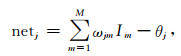
不同层的神经元由权值连接,每个神经元带有一个阈值θ.第一隐含层节点输入为
|
(1) |
其中Im为输入层第m个神经元的输入值,θj为第一隐含层第j个神经元阈值,ωjm表示第一隐含层第j个神经元与输入层第m个神经元之间的连接权值,netj表示第一隐含层第j个神经元的输入值.第一隐含层第j个神经元输出为hj=f(netj),其中f为激活函数,一般选择S型函数,函数形式为f(x)=1/(1+e-x).
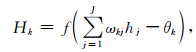
第一隐含层输出即为第二隐含层输入,进而可以得到第二隐含层输出为
|
(2) |
其中hj为第一隐含层第j个神经元的输出值,θk为第二隐含层第k个神经元阈值,ωkj表示第二隐含层第k个神经元与第一隐含层第j个神经元之间的连接权值,Hk表示第二隐含层第k个神经元的输出值.
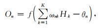
Hk作为输出层的输入,得到最终预测输出
|
(3) |
其中Hk为第二隐含层第k个神经元的输出值,θn为输出层第n个神经元阈值,ωnk表示输出层第n个神经元与第二隐含层第k个神经元之间的连接权值,On表示输出层第n个神经元的最终输出值.
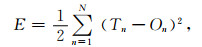
网络预测误差记为
|
(4) |
其中Tn为期望输出值,在大地电磁数据的网络学习训练中,Tn为已知模型的地电参数理论值.
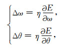
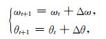
经典BP算法是采用梯度下降法修正权值和阈值,即
|
(5) |
|
(6) |
其中η为学习速率,一般取值为0.1~0.2.Δω和Δθ分别为修正的权值和阈值,ωt和θt分别为第t次迭代的权值和阈值,ωt+1和θt+1分别为第t+1次迭代的权值和阈值.通过公式(1)—(6)循环迭代,直到误差满足精度或达到设定迭代次数,网络训练结束.针对经典BP算法存在的收敛速度慢、易陷入局部最优等问题,出现了一些改进方法,如附加动量法、弹性BP算法、共轭梯度法等,本文就不再赘述.
这里需要说明的是:在大地电磁数据反演中,网络学习训练的过程为公式(1)—(6)的多次循环迭代,以获得最优的网络参数;而反演测试时只需将已训练好的网络参数即最优权值和阈值与未知模型或实测视电阻率以公式(1)—(3)进行一次计算,得到的On就是未知模型或实测数据地电参数的计算值.这种网络学习训练和反演测试分两部分进行的反演方法是神经网络反演与其他反演方法的主要不同之处,其主要计算过程和耗时在网络学习训练阶段,而将训练好的网络进行直接反演测试(只要一次计算,无需迭代),可使反演具有实时性,这也是神经网络反演的最大优势.
1.2 遗传算法优化神经网络遗传算法是基于自然选择和遗传学机理的迭代自适应概率搜索算法,具有很强的全局搜索能力,稳定性强.首先将待求解问题的各参数采用二进制(或其他编码形式)进行编码,每条染色体均包括所有参数信息,随机产生在模型空间均匀分布的初始模型群体.然后通过选择、交叉、变异一系列操作产生新一代种群.重复这一过程,使得种群不断进化,直到最优个体满足目标精度要求或达到最大遗传代数为止.
面对较复杂的非线性系统问题时,由于BP网络设置的初始权值依赖设计者的经验和样本空间的反复试验,容易产生收敛速度慢、网络不稳定以及陷入局部最优等一系列问题.将BP神经网络算法与遗传算法结合,理论上可以对任意非线性系统进行映射,并且得到全局最优的效果,从而形成一种更加有效的非线性反演方法.本文中遗传算法对BP神经网络进行如下优化:
(1) 依据待解决的问题,对网络结构进行初始化设置,确定输入层、输出层节点个数及双隐含层节点个数,分别记为M、N、H1、H2.
(2) 产生初始化种群P(t),设定遗传的种群规模,并对种群中的每个个体进行基因编码,每条染色体编码长度为N=(M×H1+H1×H2+H2×N+H1+H2+N)×L,L为变量的编码位数,包含了一个网络的所有权值和阈值信息,本文采用二进制编码.
(3) 计算种群中每一个个体的适应度,并按一定法则选取适应度好的个体组成新种群P(t).适应度函数为
(4) 将新种群中的个体随机搭配成对,对每对个体按照一定的交叉概率pc进行交叉操作,从而产生两个新的个体;并对新种群中每个个体按照设定的变异概率pm进行变异进化,产生新个体.
(5) 将产生的新个体加入到种群中,形成新种群P(t+1),群体规模不变,计算新种群中个体适应度,若满足迭代终止条件,则进行下一步,否则重复(3)—(5)步.
(6) 当达到最大遗传代数或满足误差要求时,选取最佳个体作为遗传结果,进行解码,对神经网络的连接权值和阈值进行初始赋值,然后进行网络训练,调节权值和阈值,直到满足精度要求或达到最大迭代次数,算法结束.
遗传算法优化神经网络初始权值、阈值的基本流程如图 2所示.

|
图 2 遗传算法优化神经网络流程图 Fig. 2 Flow chart of neural network optimized by genetic algorithm |
本文针对二维大地电磁TE、TM两种极化模式,分别建立了高阻异常、低阻异常、地堑以及地垒模型,考虑到计算量的问题,异常体和围岩的电阻率值不变,只通过改变异常体位置获得用于网络训练和反演测试的二维数据,以异常体中心点为基准点(地垒、地堑模型以上凸、下凹中心点为准),水平方向移动范围为-4 km到4 km,垂直方向移动范围为-2 km到-6 km,移动间距均为1 km,TE、TM两种模式下各生成180组视电阻率数据,共360组数据.将其中170组分别进行TE模式、TM模式以及TE&TM联合模式的学习训练,余下的10组作为未知模型(也叫测试模型)进行相应的反演测试.正演方法采用有限单元法,网格大小为30×31,水平方向两端各7个网格单元延伸,底部9个单元延伸,TE模式下含8个空气层.计算中选取17个测点,测点间距为1000 m,采用16个记录频点,范围为0.016~512 Hz,按对数等间隔分布.基准点样本地电模型如图 3所示.

|
图 3 基准点样本地电模型 (a)低阻异常; (b)高阻异常; (c)地堑; (d)地垒. Fig. 3 Sketch of datum sample geoelectric models (a) Low-resistivity anomaly; (b) High-resistivity anomaly; (c) Graben; (d) Horst. |
本文的建模方式是将采集频率范围内测量的所有视电阻率作为输入参数,因此TE、TM模式时网络输入参数为17×16,即272个,TE&TM联合模式时,将TE和TM两种模式下的视电阻率全部作为输入,此时输入参数为544个.所有网格的电性参数即电阻率值作为输出,由于空气层电阻率恒定,网格外延区域电阻率值取真实值,均不参与反演,因此最后的反演网格为16×22,输出参数为352个.
2.2 网络学习训练本文采用三层BP神经网络模型,输入节点为272(TE&TM联合模式时输入节点为544),输出节点为352,隐含层数为2,各隐含层节点数目按经验和试错法进行选取,确定双隐含层节点分别为12和8,训练算法选择弹性BP算法,设置训练目标拟合差(即均方误差,见公式(7))为0.1,网络的最大迭代次数为1000次.如果某次网络训练迭代次数达到了1000次,而迭代拟合差仍大于0.1,则该次训练不成功.
遗传算法优化神经网络参数设置如下:种群规模30,遗传代沟为0.95,交叉概率为0.7,变异概率为0.01,最大遗传代数为20代.对建立的三层神经网络的不同层神经元之间连接权值及隐含层阈值、输出层阈值进行二进制编码,得到一个个体的编码染色体,基因长度为65480(TE&TM联合模式时基因长度为98120).选择算子采用随机遍历抽样,交叉算子采用高级重组算子.
将神经网络算法和遗传神经网络算法分别对已知模型(170组)进行学习训练,由于一次训练过程不具有代表性,通过多组实验(每组实验进行100次网络训练),取其中10组TE&TM联合模式的数据进行对比(其中BP代表BP神经网络算法,GA-BP代表遗传神经网络算法,以下同),对比结果见表 1.可见在10组实验中,BP算法平均成功率为76%,平均运行时间为9.92 s(计算机配置:内存4 GB、CPU速度2.2 GHz、双核,以下同),而GA-BP算法平均成功率为93%,平均运行时间为8.87 s,说明通过遗传算法优化BP神经网络的初始权值和阈值,在一定程度上提高了网络收敛成功率和收敛效率.
|
|
表 1 10组实验的训练结果对比 Table 1 Comparison of training results from 10 sets of experiments |
本文就大地电磁TE模式、TM模式以及TE&TM联合模式对测试模型进行反演测试.反演测试样本为高阻、地堑及高低阻组合模型,设定反演结果与模型参数的均方误差为

|
(7) |
其中λT为归一化后的测试模型地电参数理论值,λC为归一化后的该模型反演参数计算值,N为参数个数,在本次网络反演中为352.本文对反演结果进行了BP反演与GA-BP反演对比,以及GA-BP反演与最小二乘法正则化反演对比.
2.3.1 BP反演与GA-BP反演对比用于反演测试的高阻异常体模型和地堑模型如图 4所示.高阻模型背景区域电阻率值为100 Ωm,高阻异常体电阻率为500 Ωm,水平方向范围为-3 km到3 km,垂直延伸为-1 km到-3 km.地堑模型凹陷部分电阻率为100 Ωm,深度由-1 km到-3 km,水平范围为-3 km到3 km,深部电阻率为500 Ωm.

|
图 4 反演测试模型 (a)高阻异常; (b)地堑. Fig. 4 Sketch of geoelectric model for inversion (a) High-resistivity anomaly; (b) Graben. |
图 5和图 6分别为高阻异常模型的反演结果和视电阻率对比;图 7和图 8分别为地堑模型的反演结果和视电阻率对比.图 5和图 7显示在不同反演模式下,GA-BP反演比BP反演结果的异常区域边界更为清晰;TE、TM及TE&TM联合模式均得到了良好的反演效果,相比于单一模式反演,TE&TM联合反演所得均方误差值有所减小,反演所得电阻率值更接近真实模型.由图 6和图 8可见模型理论视电阻率与GA-BP反演拟合视电阻率也基本一致.具体的反演均方误差对比见表 2.

|
图 5 高阻异常模型反演结果对比 (a) TE模式BP反演结果; (b) TE模式GA-BP反演结果; (c) TM模式BP反演结果; (d) TM模式GA-BP反演结果; (e) TE&TM联合模式BP反演结果; (f) TE&TM联合模式GA-BP反演结果. Fig. 5 Comparison of inversion results on high-resistivity anomaly model (a) BP inversion for TE mode; (b) GA-BP inversion for TE mode; (c) BP inversion for TM mode; (d) GA-BP inversion for TM mode; (e) BP inversion for TE and TM modes; (f) GA-BP inversion for TE and TM modes. |

|
图 6 高阻模型理论视电阻率与GA-BP反演拟合视电阻率对比 (a) TE模式理论视电阻率; (b) TE模式拟合视电阻率; (c) TM模式理论视电阻率; (d) TM模式拟合视电阻率. Fig. 6 Comparison between theoretical apparent resistivity and apparent resistivity from GA-BP inversion on high-resistivity model (a) Theoretical apparent resistivity of TE mode; (b) Calculated apparent resistivity of TE mode; (c)Theoretical apparent resistivity of TM mode; (d) Calculated apparent resistivity of TM mode. |

|
图 7 地堑模型反演结果对比 (a) TE模式BP反演结果; (b) TE模式GA-BP反演结果; (c) TM模式BP反演结果; (d) TM模式GA-BP反演结果; (e) TE&TM联合模式BP反演结果; (f) TE&TM联合模式GA-BP反演结果. Fig. 7 Comparison of inversion results on graben model (a) TE mode inversion using BP algorithm; (b) TE mode inversion using GA-BP algorithm; (c) TM mode inversion using BP algorithm; (d) TM mode inversion using GA-BP algorithm; (e) TE&TM mode inversion using BP algorithm; (f) TE&TM mode inversion using GA-BP algorithm. |

|
图 8 地堑模型理论视电阻率与GA-BP反演拟合视电阻率对比 (a) TE模式理论视电阻率; (b) TE模式拟合视电阻率; (c) TM模式理论视电阻率; (d) TM模式拟合视电阻率. Fig. 8 Comparison between theoretical apparent resistivity and apparent resistivity from GA-BP inversion on graben model (a) Theoretical apparent resistivity of TE mode; (b) Calculated apparent resistivity of TE mode; (c) Theoretical apparent resistivity of TM mode; (d) Calculated apparent resistivity of TM mode. |
|
|
表 2 不同反演方法和模式下均方误差对比 Table 2 Comparison of mean square errors of various inversion methods and modes |
建立二维高、低阻异常体组合模型如图 9a所示,背景区域电阻率值为300 Ωm,左侧为低阻体,大小为2000 m×2000 m,电阻率为100 Ωm,右侧为高阻体,大小与左侧一致,电阻率为500 Ωm.图 9b、图 9c分别为GA-BP的TE&TM联合反演结果和最小二乘正则化联合反演结果,异常体实际位置用虚线标出,对比两图可以看出,两异常体的位置、大小均较为明显.GA-BP反演测试运行时间为0.08 s,反演结果与模型参数的均方误差为0.0693;最小二乘正则化联合反演时,反演迭代次数为12次,程序运行时间为61.74 s,反演结果与模型参数的均方误差为0.0799.由此可见GA-BP反演具有实时性,与最小二乘正则化反演相比,反演效率得到了很大提高.由于网络训练的模型中只有单个的高阻异常或低阻异常,而反演测试中对高低阻异常也能有较好的反映,说明该反演方法对未训练的模型类型具有一定自学习能力.

|
图 9 组合模型及反演结果对比 (a)理论模型; (b) GA-BP反演结果; (c)最小二乘正则化反演结果. Fig. 9 Combined model and comparison of inversion results (a) Theoretical model; (b) GA-BP inversion result; (c) Least squares regularization inversion result. |
实测数据来自云南省白牛厂矿区某测线,野外采用EH4电导率成像仪进行数据采集.该矿区中,铅锌矿、浸染状矿石的电阻率为100~600 Ωm,围岩的电阻率均在1000 Ωm以上,本测线有测点51个,点距40 m.根据矿区已知地质资料和岩矿石标本物性测定结果,以及实测视电阻率数据,构建适合本地区的多种地质模型进行遗传神经网络训练,网络参数与模型实验一致,将学习训练好的网络进行实测数据的TE&TM联合模式反演测试,并将该反演结果与经典的最小二乘正则化反演进行对比.
图 10为实测视电阻率与GA-BP反演拟合视电阻率对比图,可以看出拟合的视电阻率与实测视电阻率一致性较好.图 11a、11b分别为实测资料的GA-BP反演结果与最小二乘正则化反演结果.钻孔资料(ZK1、ZK2)显示,该矿区主要有白云岩、大理岩、矽化岩层、花岗岩等岩性,其中含矿层为大理岩,矽化岩层与花岗岩交界面电阻率为200~500 Ωm,相比最小二乘反演,GA-BP反演电性变化趋势大体一致,推断的含矿层分界线用红色曲线标识,该反演结果与钻孔资料基本一致,可为该地区具有一定规模的隐伏矿体的赋存空间的宏观预测提供比较可靠的依据.最小二乘正则化反演时,程序运行时间为138.61 s;而GA-BP反演时,十次平均学习训练时间为29.28 s,反演测试时间为0.14 s,可见GA-BP反演极大提高了反演效率.

|
图 10 实测视电阻率(a)与GA-BP反演拟合视电阻率(b)对比 Fig. 10 Measured apparent resistivity (a) and calculated apparent resistivity from GA-BP inversion (b) |

|
图 11 GA-BP反演(a)与最小二乘正则化反演(b)电阻率剖面对比 Fig. 11 Comparison of resistivity sections of GA-BP inversion (a) and least squares regularization inversion (b) |
(1) 通过合理的设计网络输入层、隐含层及输出层参数,构建大地电磁神经网络结构,对网络进行学习训练,训练好的网络能基本准确地反映大地电磁非线性反演特性,取得较好的反演效果;
(2) 本反演方法分为学习训练与反演测试两个过程,由于网络的学习训练对时效性要求不高,训练好的网络可直接用于大地电磁非线性反演,可使反演具有实时性,相比经典的最小二乘反演,极大提高了反演效率;
(3) 遗传算法对神经网络进行权值和阈值的优化,充分利用了遗传算法的全局寻优性和神经网络的局部寻优性,使网络训练的收敛成功率和计算速度得到提高,反演测试结果也更精确;
(4) 由于三维模型涉及的数据量过大、模型更加复杂,怎样进行网络结构的优化和数据的选取还需要进一步深入研究.
致谢特别感谢两位评审专家为本文提出的宝贵修改意见,感谢编辑对本文修改给予的帮助.
Ahmadi M A, Zendehboudi S, Lohi A, et al.
2013. Reservoir permeability prediction by neural networks combined with hybrid genetic algorithm and particle swarm optimization. Geophysical Prospecting, 61(3): 582-598.
DOI:10.1111/gpr.2013.61.issue-3 |
|
Aleardi M.
2015. Seismic velocity estimation from well log data with genetic algorithms in comparison to neural networks and multilinear approaches. Journal of Applied Geophysics, 117: 13-22.
DOI:10.1016/j.jappgeo.2015.03.021 |
|
Avdeev D, Avdeeva A.
2009. 3D magnetotelluric inversion using a limited-memory quasi-Newton optimization. Geophysics, 74(3): F45-F57.
DOI:10.1190/1.3114023 |
|
Beka T I, Smirnov M, Birkelund Y, et al.
2016. Analysis and 3D inversion of magnetotelluric crooked profile data from central Svalbard for geothermal application. Tectonophysics, 686: 98-115.
DOI:10.1016/j.tecto.2016.07.024 |
|
Chen X B, Zhao G Z, Tang J, et al.
2005. An adaptive regularized inversion algorithm for magnetotelluric data. Chinese Journal of Geophysics, 8(4): 937-946.
|
|
Constable S C, Parker R L, Constable C G.
1987. Occam's inversion:a practical algorithm for generating smooth models from electromagnetic sounding data. Geophysics, 52(3): 289-300.
DOI:10.1190/1.1442303 |
|
Dai Q W, Jiang F B.
2013. Nonlinear inversion for electrical resistivity tomography based on chaotic oscillation PSO-BP algorithm. The Chinese Journal of Nonferrous Metals, 23(10): 2897-2904.
|
|
Dai Q W, Jiang F B, Dong L.
2014. RBFNN inversion for electrical resistivity tomography based on Hannan-Quinn criterion. Chinese Journal of Geophysics, 57(4): 1335-1344.
DOI:10.6038/cjg20140430 |
|
De Groot-Hedlin C, Constable S.
1993. Occam's inversion and the North American Central Plains electrical anomaly. Journal of Geomagnetism and Geoelectricity, 45(9): 985-999.
DOI:10.5636/jgg.45.985 |
|
De Groot-Hedlin C, Constable S.
2004. Inversion of magnetotelluric data for 2D structure with sharp resistivity contrasts. Geophysics, 69(1): 78-86.
DOI:10.1190/1.1649377 |
|
Dittmer J K, Szymanski J E.
1995. The stochastic inversion of magnetics and resistivity data using the simulated annealing algorithm. Geophysical Prospecting, 43(3): 397-416.
DOI:10.1111/gpr.1995.43.issue-3 |
|
Dong H, Wei W B, Ye G F, et al.
2014. Study of three-dimensional magnetotelluric inversion including surface topography based on finite-difference method. Chinese Journal of Geophysics, 57(3): 939-952.
DOI:10.6038/cjg20140323 |
|
El-Qady G, Ushijima K.
2001. Inversion of DC resistivity data using neural networks. Geophysical Prospecting, 49(4): 417-430.
DOI:10.1046/j.1365-2478.2001.00267.x |
|
Feng D S, Wang X.
2013. Magnetotelluric finite element method forward based on biquadratic interpolation and least squares regularization joint inversion. The Chinese Journal of Nonferrous Metals, 23(9): 2524-2531.
DOI:10.1016/S1003-6326(13)62764-8 |
|
Han Q, Hu X Y, Cheng Z P, et al.
2015. A study of two-dimensional MT inversion with steep topography using the adaptive unstructured finite element method. Chinese Journal of Geophysics, 58(12): 4675-4684.
DOI:10.6038/cjg20151228 |
|
Hu X Y, Li Y, Yang W C, et al.
2012. Three-dimensional magnetotelluric parallel inversion algorithm using data space method. Chinese Journal of Geophysics, 55(12): 3969-3978.
DOI:10.6038/j.issn.0001-5733.2012.12.009 |
|
Hu Z Z, Hu X Y, He Z X.
2006. Pseudo-three-dimensional magnetotelluric inversion using nonlinear conjugate gradients. Chinese Journal of Geophysics, 49(4): 1226-1234.
|
|
Hu Z Z, Chen Y, He Z X, et al.
2010. MT parallel simulated annealing constrained inversion and its application. Oil Geophysical Prospecting, 45(4): 597-601, 624.
|
|
Hu Z Z, He Z X, Yang W C, et al.
2015. Constrained inversion of magnetotelluric data with the artificial fish swarm optimization method. Chinese Journal of Geophysics, 58(7): 2578-2587.
DOI:10.6038/cjg20150732 |
|
Lee S K, Kim H J, Song Y, et al.
2009. MT2DInvMatlab-A program in MATLAB and FORTRAN for two-dimensional magnetotelluric inversion. Computers & Geosciences, 35(8): 1722-1734.
|
|
Lin C H, Tan H D, Tong T.
2009. Parallel rapid relaxation inversion of 3D magnetotelluric data. Applied Geophysics, 6(1): 77-83.
DOI:10.1007/s11770-009-0010-5 |
|
Lin C H, Tan H D, Tong T.
2011. Three-dimensional conjugate gradient inversion of magnetotelluric full information data. Applied Geophysics, 8(1): 1-10.
DOI:10.1007/s11770-010-0266-9 |
|
Liu B, Li S C, Nie L C, et al.
2012. 3D resistivity inversion using an improved Genetic Algorithm based on control method of mutation direction. Journal of Applied Geophysics, 87: 1-8.
DOI:10.1016/j.jappgeo.2012.08.002 |
|
Liu B, Liu Z Y, Song J, et al.
2017. Joint inversion method of 3D electrical resistivity detection based on inequality constraints. Chinese Journal of Geophysics, 60(2): 820-832.
DOI:10.6038/cjg20170232 |
|
Liu J F, Hu W B, Hu X Y.
2015. Two-dimensional magnetotelluric inversion using differential ant-stigmergy algorithm. Oil Geophysical Prospecting, 50(3): 548-555.
|
|
Liu J X, Tong X Z, Yang X H, et al.
2008. Application of real coded genetic algorithm in two-dimensional magnetotelluric inversion. Progress in Geophysics, 23(6): 1936-1942.
|
|
Luo H M, Wang J Y, Zhu P M, et al.
2009. Quantum genetic algorithm and its application in magnetotelluric data inversion. Chinese Journal of Geophysics, 52(1): 260-267.
DOI:10.1002/cjg2.v52.1 |
|
Mackie R L, Madden T R.
1993. Three-dimensional magnetotelluric inversion using conjugate gradients. Geophysical Journal International, 115(1): 215-229.
DOI:10.1111/gji.1993.115.issue-1 |
|
Majdi A, Beiki M.
2010. Evolving neural network using a genetic algorithm for predicting the deformation modulus of rock masses. International Journal of Rock Mechanics and Mining Sciences, 47(2): 246-253.
DOI:10.1016/j.ijrmms.2009.09.011 |
|
Montahaei M, Oskooi B.
2014. Magnetotelluric inversion for azimuthally anisotropic resistivities employing artificial neural networks. Acta Geophysica, 62(1): 12-43.
DOI:10.2478/s11600-013-0164-7 |
|
Newman G A, Alumbaugh D L.
2000. Three-dimensional magnetotelluric inversion using non-linear conjugate gradients. Geophysical Journal International, 140(2): 410-424.
DOI:10.1046/j.1365-246x.2000.00007.x |
|
Oskooi B, Darijani M.
2014. 2D inversion of the magnetotelluric data from Mahallat geothermal field in Iran using finite element approach. Arabian Journal of Geosciences, 7(7): 2749-2759.
DOI:10.1007/s12517-013-0893-6 |
|
Pérez-Flores M A, Schultz A.
2002. Application of 2-D inversion with genetic algorithms to magnetotelluric data from geothermal areas. Earth, Planets and Space, 54(5): 607-616.
DOI:10.1186/BF03353049 |
|
Rodi W, Mackie R L.
2001. Nonlinear conjugate gradients algorithm for 2-D magnetotelluric inversion. Geophysics, 66(1): 174-187.
DOI:10.1190/1.1444893 |
|
Sarvandani M M, Kalateh A N, Unsworth M, et al.
2017. Interpretation of magnetotelluric data from the Gachsaran oil field using sharp boundary inversion. Journal of Petroleum Science and Engineering, 149: 25-39.
DOI:10.1016/j.petrol.2016.10.019 |
|
Sasaki Y.
2004. Three-dimensional inversion of static-shifted magnetotelluric data. Earth, Planets and Space, 56(2): 239-248.
DOI:10.1186/BF03353406 |
|
Shaw R, Srivastava S.
2007. Particle swarm optimization:A new tool to invert geophysical data. Geophysics, 72(2): F75-F83.
DOI:10.1190/1.2432481 |
|
Shi X M, Wang J Y.
1998. One dimensional magnetotelluric sounding inversion using simulated annealing. Earth Science-Journal of China University of Geosciences, 23(5): 542-546.
|
|
Shi X M, Wang J Y, Zhang S Y, et al.
2000. Multiscale genetic algorithm and its application in magnetotelluric sounding data inversion. Chinese Journal of Geophysics, 43(1): 122-130.
|
|
Shimelevich M I, Obornev M A, Gavryushov S.
2007. Rapid neuronet inversion of 2D magnetotelluric data for monitoring of geoelectrical section parameters. Annals of Geophysics, 50(1): 105-109.
|
|
Siripunvaraporn W, Egbert G.
2000. An efficient data-subspace inversion method for 2-D magnetotelluric data. Geophysics, 65(3): 791-803.
DOI:10.1190/1.1444778 |
|
Siripunvaraporn W, Egbert G.
2007. Data space conjugate gradient inversion for 2-D magnetotelluric data. Geophysical Journal International, 170(3): 986-994.
DOI:10.1111/gji.2007.170.issue-3 |
|
Siripunvaraporn W.
2012. Three-dimensional magnetotelluric inversion:an introductory guide for developers and users. Surveys in Geophysics, 33(1): 5-27.
DOI:10.1007/s10712-011-9122-6 |
|
Smith J T, Booker J R.
1991. Rapid inversion of two-and three-dimensional magnetotelluric data. Journal of Geophysical Research:Solid Earth, 96(B3): 3905-3922.
DOI:10.1029/90JB02416 |
|
Smith T, Hoversten M, Gasperikova E, et al.
1999. Sharp boundary inversion of 2D magnetotelluric data. Geophysical Prospecting, 47(4): 469-486.
DOI:10.1046/j.1365-2478.1999.00145.x |
|
Spichak V, Popova I.
2000. Artificial neural network inversion of magnetotelluric data in terms of three-dimensional earth macroparameters. Geophysical Journal International, 142(1): 15-26.
DOI:10.1046/j.1365-246x.2000.00065.x |
|
Tan H D, Yu Q F, Booker J, et al.
2003. Three-dimensional rapid relaxation inversion for the magnetotelluric method. Chinese Journal of Geophysics, 46(6): 850-854, 889.
|
|
Tong X Z. 2008. Research of forward using finite element method and regularized inversion using hybrid genetic algorithm in magnetotelluric sounding (in Chinese). Changsha: Central South University.
|
|
Wang H, Jiang H, Wang L, et al.
2015. Magnetotelluric inversion using artificial neural network. Journal of Central South University (Science and Technology), 46(5): 1707-1714.
|
|
Xiao M. 2010. Two-dimensional magnetotelluric inversion using particle swarm optimization algorithm (in Chinese). Wuhan: China University of Geosciences.
|
|
Xu Y X, Wang J Y.
1998. A multiresolution inversion of one-dimensional magnetotelluric data. Chinese Journal of Geophysics, 41(5): 704-711.
|
|
Yan L J, Hu W B.
2004. Non-linear inversion with the quadratic function approaching method for magnetotelluric data. Chinese Journal of Geophysics, 47(5): 935-940.
|
|
Yi Y Y, Wang J Y.
2009. Lecture on non-linear inverse methods in geophysical data (10) particle swarm optimization inversion method. Chinese Journal of Engineering Geophysics, 6(4): 385-389.
|
|
陈小斌, 赵国泽, 汤吉, 等.
2005. 大地电磁自适应正则化反演算法. 地球物理学报, 48(4): 937–946.
|
|
戴前伟, 江沸菠.
2013. 基于混沌振荡PSO-BP算法的电阻率层析成像非线性反演. 中国有色金属学报, 23(10): 2897–2904.
|
|
戴前伟, 江沸菠, 董莉.
2014. 基于汉南-奎因信息准则的电阻率层析成像径向基神经网络反演. 地球物理学报, 57(4): 1335–1344.
DOI:10.6038/cjg20140430 |
|
董浩, 魏文博, 叶高峰, 等.
2014. 基于有限差分正演的带地形三维大地电磁反演方法. 地球物理学报, 57(3): 939–952.
DOI:10.6038/cjg20140323 |
|
冯德山, 王珣.
2013. 大地电磁双二次插值FEM正演及最小二乘正则化联合反演. 中国有色金属学报, 23(9): 2524–2531.
|
|
韩骑, 胡祥云, 程正璞, 等.
2015. 自适应非结构有限元MT二维起伏地形正反演研究. 地球物理学报, 58(12): 4675–4684.
DOI:10.6038/cjg20151228 |
|
胡祥云, 李焱, 杨文采, 等.
2012. 大地电磁三维数据空间反演并行算法研究. 地球物理学报, 55(12): 3969–3978.
DOI:10.6038/j.issn.0001-5733.2012.12.009 |
|
胡祖志, 胡祥云, 何展翔.
2006. 大地电磁非线性共轭梯度拟三维反演. 地球物理学报, 49(4): 1226–1234.
|
|
胡祖志, 陈英, 何展翔, 等.
2010. 大地电磁并行模拟退火约束反演及应用. 石油地球物理勘探, 45(4): 597–601, 624.
|
|
胡祖志, 何展翔, 杨文采, 等.
2015. 大地电磁的人工鱼群最优化约束反演. 地球物理学报, 58(7): 2578–2587.
DOI:10.6038/cjg20150732 |
|
刘斌, 刘征宇, 宋杰, 等.
2017. 基于不等式约束的三维电阻率探测混合反演方法. 地球物理学报, 60(2): 820–832.
DOI:10.6038/cjg20170232 |
|
刘剑锋, 胡文宝, 胡祥云.
2015. 二维大地电磁资料的差分蚁群法反演. 石油地球物理勘探, 50(3): 548–555.
|
|
柳建新, 童孝忠, 杨晓弘, 等.
2008. 实数编码遗传算法在大地电磁测深二维反演中的应用. 地球物理学进展, 23(6): 1936–1942.
|
|
罗红明, 王家映, 朱培民, 等.
2009. 量子遗传算法在大地电磁反演中的应用. 地球物理学报, 52(1): 260–267.
|
|
师学明, 王家映.
1998. 一维层状介质大地电磁模拟退火反演法. 地球科学——中国地质大学学报, 23(5): 542–546.
|
|
师学明, 王家映, 张胜业, 等.
2000. 多尺度逐次逼近遗传算法反演大地电磁资料. 地球物理学报, 43(1): 122–130.
|
|
谭捍东, 余钦范, BookerJ, 等.
2003. 大地电磁法三维快速松弛反演. 地球物理学报, 46(6): 850–854, 889.
|
|
童孝忠. 2008. 大地电磁测深有限单元法正演与混合遗传算法正则化反演研究. 长沙: 中南大学.
|
|
王鹤, 蒋欢, 王亮, 等.
2015. 大地电磁人工神经网络反演. 中南大学学报(自然科学版), 46(5): 1707–1714.
DOI:10.11817/j.issn.1672-7207.2015.05.019 |
|
肖敏. 2010. 二维大地电磁粒子群优化算法反演方法研究. 武汉: 中国地质大学.
|
|
徐义贤, 王家映.
1998. 大地电磁的多尺度反演. 地球物理学报, 41(5): 704–711.
|
|
严良俊, 胡文宝.
2004. 大地电磁测深资料的二次函数逼近非线性反演. 地球物理学报, 47(5): 935–940.
|
|
易远元, 王家映.
2009. 地球物理资料非线性反演方法讲座(十)——粒子群反演方法. 工程地球物理学报, 6(4): 385–389.
|
|