 2018, Vol. 61


2. 非常规油气湖北协同创新中心, 武汉 430100;
3. 长江大学地球物理与石油资源学院, 武汉 430100;
4. 中石化地球物理公司华东分公司, 南京 211112;
5. 中国科学院地质与地球物理研究所, 中国科学院地球与行星物理重点实验室, 北京 100029;
6. 美国加州大学圣克鲁兹分校地球物理与行星物理研究所, 圣克鲁兹 95064
2. Hubei Cooperative Innovation Center of Unconventional Oil and Gas, Wuhan 430100, China;
3. School of Geophysics and Oil Resources, Yangtze University, Wuhan 430100, China;
4. Sinopec Geophysical Corporation Huadong Branch, Nanjing 211112, China;
5. Key Laboratory of Earth and Planetary Physics, Institute of Geology and Geophysics, Chinese Academy of Sciences, Beijing 100029, China;
6. Institute of Geophysics and Planetary Physics, University of California at Santa Cruz 95064, California, USA
频率域有限差分正演模拟可用于全波形反演和逆时偏移,在地震波场模拟中占有重要地位(e.g. Pratt, 1999; Brossier et al., 2009; Virieux and Operto, 2009; Loewenthal and Mufti, 1983; Plessix and Mulder, 2004; Kim et al., 2011).相比于时间域模拟,具有无时间频散和累积误差,适合多炮并行运算,频带选取灵活,易于模拟非弹性效应等优点.Pratt和Worthington(1990)基于2D声波方程提出了经典的5点频率域有限差分格式,但是数值频散严重.为提高计算精度,基于旋转坐标的FD格式被广泛应用(e.g. Jo et al., 1996; Shin and Sohn, 1998; Štekl and Pratt, 1998; Hustedt et al., 2004; Operto et al., 2007, 2009, 2014; 曹书红和陈景波, 2012).Jo等(1996)利用0°和45°方向的组合差分近似拉普拉斯算子,对2D声波方程提出了优化9点差分格式,频散曲线得到较大的改进.之后,Operto等(2007)将其扩展至基于3D黏弹性声波方程的27点格式.但是旋转坐标的FD格式只适用于空间横纵向等间隔采样的情况,使得此种方法在实际波场模拟中受限.为了适应长方形网格的模拟,平均导数法(ADM, average-derivative method)应运而生(Chen, 2012;张衡等, 2014; Zhang et al., 2015;Tang et al. 2015;Chen and Cao, 2016).Chen(2012)对2D声波方程提出了基于平均导数法的优化9点格式,这种格式包含了旋转9点格式.之后Chen (2014)将其扩展至3D声波情况.以上基于旋转坐标的优化格式均是对应基于平均导数法优化格式的一种特殊形式,理论上平均导数优化格式的精度要优于相应的旋转坐标优化格式.
在时间域有限差分正演算法中,往往存在一般性通用的FD算子系数确定方法(e.g. Holberg, 1987; Liu and Sen, 2009; Chu and Stoffa, 2012; Zhang and Yao, 2012, 2013).只要给定FD算子的模板,就能利用最优化的频散关系确定每个FD模板节点上对应的系数.而目前基于2D声波方程频率域FD算子格式有多种,比如9点,15点,17点,25点等各种格式的算法,其对应的算子系数确定方法也各不相同(e.g. Jo et al., 1996; Min et al., 2000; Chen, 2012; 张衡等, 2014; 刘璐等, 2013; Tang et al., 2015; Gu et al., 2013).Fan等(2017)基于2D声波方程提出了一个适用性较广的优化方法,此方法几乎可以优化2D情况下的各种差分格式.本文将Fan等(2017)提出的2D频率域优化方法扩展至3D声波情况.只要给定3D的FD模板格式,便可利用此方法求解出对应的优化系数.
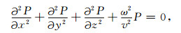
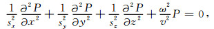
1 理论 1.1 差分格式频率域三维声波方程可写为
|
(1) |
其中,P是位移分量,ω是角频率,v是声波速度.
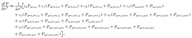
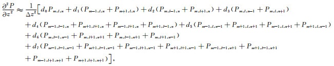
假设周围几个点的波场值对中心点二阶空间导数的近似都有一定程度的贡献,且到中心点距离相等的点权值大小相等.我们首先采用以下常用的3D 27点格式近似空间导数(图 1):

|
图 1 频率域三维有限差分算子 Fig. 1 Grid configurations for 3D frequency-domain FD operator |
|
(2a) |

|
(2b) |
|
(2c) |
式中,Pm, l, n=P(mΔx, lΔy, nΔz),Δx、Δy和Δz分别是x、y和z方向的空间采样间隔,ci、ei、di分别表示不同距离的点对

|
(3a) |

|
(3b) |

|
(3c) |
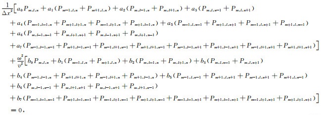
对于质量加速度项

|
(4) |
式中,bi表示不同距离的点对平均质量加速项

|
(5) |
27点差分格式(4)实际上是一种通用的格式,其他常见的3D差分格式包括经典的7点格式和ADM 27点格式均是差分格式(4)的一种特殊形式,其对比关系详见附录.
我们首先考虑Δx=max(Δx, Δy, Δz)的情况,对于其他两种的情况后续进行讨论.将采样间隔比r1=Δx/Δy、r2=Δx/Δz代入式(4),并令

|
(6) |
得到:
|
(7) |
其中,

|
(8) |
式(7)成为简化后最终的27点差分格式,式中仅有14个相互独立的系数.
1.2 频散分析
采用经典的频散分析方法,将平面波P(x, y, z, ω)=

|
(9) |
式中,Vph是相速度,
|
|
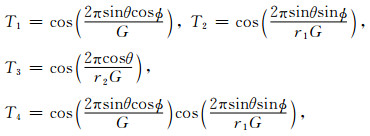
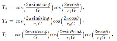
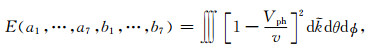
每波长的采样点数G与最大采样间隔max(Δx, Δy, Δz)有关.对于Δx=max(Δx, Δy, Δz)的情况G=2π/(kΔx).θ是声波传播方向与z方向的夹角,ϕ是方位角,即传播方向的水平投影量与x方向的夹角,满足关系式kx=ksinθcosϕ, ky=ksinθsinϕ, kz=kcosθ.最小化以下相速度误差函数即可求取14个独立系数ai, bi(i=1, 2, …, 7)的值,
|
(10) |
其中,

采用目前使用广泛的PML吸收边界条件.PML层内部的频率域声波方可写为(Tang et al., 2015; Fan et al., 2017):
|
(11) |
其中,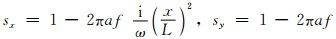

|
(12a) |

|
(12b) |

|
(12c) |
则最小化以下目标函数即可求取ci、ei、di的值
|
(13) |
式中,
对于27点格式,首先通过优化式(10)求取ai和bi(i=1, 2, …, 7)的值,然后通过优化式(13)求取ci、di、ei(i=1, 2, …, 7)的值,整个过程中总共需要确定28个独立的系数.我们采用MATLAB软件中的约束非线性最优化函数fmincon求取式(10)和(13)中的优化系数.传播角度θ和ϕ取值范围均为[0, π/2],间隔为π/200.

|
图 2 ADM 27点格式和本文优化27点格式频散曲线对比 左列是ADM 27点格式,右列是本文优化27点格式,每行子图对应不同的空间采样比,(a, b) r1=1.0,r2=1.0; (c, d) r1=1.0,r2=2.0; (e, f) r1=1.0,r2=3.0; (g, h) r1=2.0,r2=1.0; (i, j) r1=2.0,r2=2.0; (k, l) r1=2.0,r2=3.0.子图中不同颜色的曲线代表各种不同的传播方向,传播角度θ和ϕ取值范围[0, π/2],采样间隔为π/20. Fig. 2 Normalized phase velocity curves for the ADM 27-point scheme (left column) and our optimal 27-point scheme (right column) Rows from top to bottom are for r1=1.0 and r2=1.0 (a, b), r1=1.0 and r2=2.0 (c, d), r1=1.0 and r2=3.0 (e, f), r1=2.0 and r2=1.0 (g, h), r1=2.0 and r2=2.0 (i, j), r1=2.0 and r2=3.0 (k, l). The colorful curves denote the different propagation directions. The ranges of propagation angles θ and ϕ are both within [0, π/2] at an interval of π/20. |
|
|
表 1 当Δx=max(Δx, Δy, Δz)时,不同r1和r2情况下27点格式的优化系数 Table 1 Optimized coefficients for 27-point scheme with different r1, r2 values and Δx= max(Δx, Δy, Δz) |
前面只考虑了Δx=max(Δx, Δy, Δz)的情况,对于Δy=max(Δx, Δy, Δz)和Δz=max(Δx, Δy, Δz)的情况,由于27点格式具有几何对称性,Δx=max(Δx, Δy, Δz)情况下ai(i=1, 2, …, 7)的值若按顺序赋给a2、a3、a1、a6、a4、a5、a7即可得到Δy=max(Δx, Δy, Δz)情况下的优化系数,若按顺序赋给a3、a1、a2、a5、a6、a4、a7即可得到Δz=max(Δx, Δy, Δz)情况下的优化系数.
优化方法除了能优化27点格式,也能优化其他3D频率域有限差分格式,比如7点格式.设定

|
图 3 经典的7点格式和本文优化7点格式频散曲线对比 左列是经典的7点格式,右列是本文优化7点格式,每行子图对应不同的空间采样比;(a, b) r1=1.0,r2=1.0; (c, d) r1=1.0,r2=2.0; (e, f) r1=1.0,r2=3.0; (g, h) r1=2.0,r2=1.0; (i, j) r1=2.0,r2=2.0; (k, l) r1=2.0,r2=3.0.子图中不同颜色的曲线代表各种不同的传播方向,传播角度θ和ϕ取值范围[0, π/2],采样间隔为π/20 Fig. 3 Normalized phase velocity curves for the classical 7-point scheme (left column) and our optimal 27-point scheme (right column) Rows from top to bottom are for r1=1.0 and r2=1.0 (a, b), r1=1.0 and r2=2.0 (c, d), r1=1.0 and r2=3.0 (e, f), r1=2.0 and r2=1.0 (g, h), r1=2.0 and r2=2.0 (i, j), r1=2.0 and r2=3.0 (k, l). The colorful curves denote the different propagation directions. The ranges of propagation angles θ and ϕ are both within [0, π/2] at an interval of π/20. |
|
|
表 2 当Δx=max(Δx, Δy, Δz)时,不同r1和r2情况下7点格式的优化系数 Table 2 Optimized coefficients for 7-point scheme with different r1, r2 values and Δx=max(Δx, Δy, Δz) |
为了测试本文的27点优化格式的精度,分别采用ADM 27点格式、本文的27点格式以及解析法对一个均匀各向同性的介质模型进行正演计算,其中解析解与Chen (2014)的方法一致.模型大小为960 m×960 m×960 m,波速为3500 m·s-1,震源位于模型中心处,时间函数采用主频为30 Hz的雷克子波.模型采用正方体网格剖分,即r1=1.0,r2=1.0,网格间距Δx=Δy=Δz=16 m.图 4给出了三种方法的结果对比图,其中图 4a和4b是两种数值方法ADM 27点格式和本文的27点格式在0.16 s时刻y=480 m处xoz平面内的波场快照图,图 4c和4d分别是波场快照图在深度z=480 m处沿水平方向的横截波形图和在x=480 m处沿垂直方向的横截波形图,图中三条曲线分别对应ADM 27点格式(蓝色曲线),本文的27点格式(红色曲线)以及解析解(黑色曲线)的计算结果.其中,ADM 27点格式与本文的27点格式的波形曲线完全重合在一起,说明两者的精度基本一致,与前面的频散曲线(图 2)分析结果一致.两种数值方法与解析解的波形存在很小的差异,是由于数值误差的存在,如果采用更小的空间网格间距,数值解与解析解的波形差异将会减小.

|
图 4 均匀各向同性介质中ADM 27点格式、本文的27点格式和解析解的模拟结果对比 (a)和(b) ADM 27点格式和本文的27点格式在0.16 s时刻y=480 m处xoz平面内的波场快照图; (c)两种数值方法的波场快照图在深度z=480 m处沿水平方向的横截波形图与解析解的对比图; (d)波场快照图在x=480 m处沿垂直方向的横截波形图与解析解的对比图,图中三条不同颜色的曲线分别对应ADM 27点格式(蓝色曲线)、本文的27点格式(红色曲线)以及解析解(黑色曲线)的计算结果. Fig. 4 Simulation results for ADM 27-point scheme, our optimal 27-point scheme and analytical solution in homogenous media Panel (a) and (b) are the wavefield snapshots of ADM 27-point scheme and our optimal 27-point scheme at t=0.16 s in the xoz plane at the y=480 m. Panel (c) is the horizontal cross sections of snapshots at the depth of z=480 m comparing with analytical solution. Panel (d) is the vertical cross sections at the distance of x=480 m. The curves in three different color represent the simulation waveforms for ADM 27-point scheme (blue), our optimal 27-point scheme (red) and analytical solution (black). |
为了测试7点优化格式的精度,选取一个大小为840 m×840 m×840 m的均匀各向同性介质模型,分别采用两种方式进行网格剖分.一种是正方体网格,即r1=r2=1.0,空间采样间隔Δx=Δy=Δz=14 m.我们分别使用了经典的7点格式、本文的7点格式以及解析法进行正演计算.图 5a和5b是经典7点格式和本文的7点格式在同一时刻y=420 m处xoz平面内的波场快照图,图 5c和5d分别是波场快照图在深度z=420 m处沿水平方向的横截波形图和在x=420 m处沿垂直方向的横截波形图,图中三条曲线分别对应经典7点格式(蓝色曲线)、本文的7点格式(红色曲线)以及解析解(黑色曲线)的计算结果.可以看出两种数值方法与解析解的波形差别较大,说明均存在数值频散,但是,经典7点格式比本文的7点格式数值误差更大,其精度更低.为了减少数值误差的影响,减小空间采样间隔,分别采用Δx=Δy=Δz=10 m和Δx=Δy=Δz=8 m的网格间距,得到与图 5(c和d)类似的横截波形图(图 6,7),可以看出经典7点格式和本文的7点格式均随着采样间距的变小,数值误差变小.但是,经典7点格式比本文的7点格式的数值误差更大(图 6),说明其精度更低,当间距进一步减小,两种方法与解析解基本一致(图 7).

|
图 5 均匀各向同性介质中经典的7点格式、本文的7点格式和解析解的模拟结果对比 (a, b)经典的7点格式和本文的7点格式(r1=1.0,r2=1.0)在同一时刻y=420 m处xoz平面内的波场快照图; (c)两种数值方法的波场快照图在深度z=420 m处沿水平方向的横截波形图与解析解的对比图; (d)波场快照图在x=420 m处沿垂直方向的横截波形图与解析解的对比图,图中三条曲线分别对应经典的7点格式(蓝色曲线)、本文的7点格式(红色曲线)以及解析解(黑色曲线)的计算结果. Fig. 5 Simulation results for classical 7-point scheme, our optimal 7-point scheme and analytical solution in homogenous media Panel (a) and (b) are the wavefield snapshots of classical 7-point scheme and our optimal 7-point scheme (r1=1.0, r2=1.0) at the same time in the xoz plane at the y=420 m. Panel (c) is the horizontal cross sections of snapshots at the depth of z=420 m comparing with analytical solution. Panel (d) is the vertical cross sections at the distance of x=420 m. The curves in three different color represent the simulation waveforms for classical 7-point scheme (blue), our optimal 7-point scheme (red) and analytical solution (black). |

|
图 6 均匀各向同性介质中经典的7点格式(蓝色曲线)、本文的7点格式(红色曲线)和解析解(黑色曲线)的模拟结果对比 两种数值方法的空间采样间隔均为Δx=Δy=Δz=10 m. (a)在y=300 m、z=300 m处沿水平方向的横截波形图与解析解的对比图;(b)在x=300 m、y=300 m处沿垂直方向的横截波形图与解析解的对比图. Fig. 6 Simulation results for classical 7-point scheme (blue line), our optimal 7-point scheme (red line) and analytical solution (black line) in homogenous media The spatial intervals for two numerical methods are Δx=Δy=Δz=10 m. Panel (a) are the horizontal waveforms along the line of y=300 m, z=300 m for three methods. Panel (b) are the vertical waveforms along the line of x=300 m, y=300 m for three methods. |

|
图 7 均匀各向同性介质中经典的7点格式(蓝色曲线)、本文的7点格式(红色曲线)和解析解(黑色曲线)的模拟结果对比 两种数值方法的空间采样间隔均为Δx=Δy=Δz=8 m. (a)在y=240 m、z=240 m处沿水平方向的横截波形图与解析解的对比图; (b)在x=240 m、y=240 m处沿垂直方向的横截波形图与解析解的对比图. Fig. 7 Simulation results for classical 7-point scheme (blue line), our optimal 7-point scheme (red line) and analytical solution (black line) in homogenous media The spatial intervals for two numerical method are Δx=Δy=Δz=8 m. Panel (a) are the horizontal waveforms along the line of y=240 m, z=240 m for three methods. Panel (b) are the vertical waveforms along the line of x=240 m、y=240 m for three methods. |
另一种是长方体网格剖分地下模型,即r1=1.0,r2=2.0(Δx=max(Δx, Δy, Δz)),空间采样间隔Δx=Δy=14 m,Δz=7 m,模型网格大小为61×61×121.图 8(a, b)是经典7点格式和本文的7点格式在同一时刻y=420 m处xoz平面内的波场快照图,图 8c和8d分别是波场快照图在深度z=420 m处沿水平方向的横截波形图和在x=420 m处沿垂直方向的横截波形图,图中三条曲线分别对应经典7点格式(蓝色曲线),本文的7点格式(红色曲线)以及解析解(黑色曲线)的计算结果.由于z方向上采样间隔较小,故两种数值方法在有x方向上存在较严重的数值频散(图 8c),z方向上与解析解吻合度较高(图 8d).但是无论在x还是z方向上,本文的7点格式比经典7点格式的数值误差小,说明本文的7点格式精度更高,验证了图 3中的理论频散分析.

|
图 8 均匀各向同性介质中经典的7点格式、本文的7点格式和解析解的模拟结果对比 (a, b)经典的7点格式和本文的7点格式(r1=1.0,r2=2.0)在同一时刻y=420 m处xoz平面内的波场快照图; (c)两种数值方法的波场快照图在深度z=420 m处沿水平方向的横截波形图与解析解的对比图; (d)波场快照图在x=420 m处沿垂直方向的横截波形图与解析解的对比图,图中三条曲线分别对应经典的7点格式(蓝色曲线)、本文的7点格式(红色曲线)以及解析解(黑色曲线)的计算结果. Fig. 8 Simulation results for classical 7-point scheme, our optimal 7-point scheme and analytical solution in homogenous media Panel (a) and (b) are the wavefield snapshots of classical 7-point scheme and our optimal 7-point scheme (r1=1.0, r2=2.0) at the same time in the xoz plane at the y=420 m. Panel (c) is the horizontal cross sections of panel a and b at the depth of z=420 m comparing with analytical solution. Panel (d) is the vertical cross sections at the distance of x=420 m. The curves in three different color represent the simulation waveforms for classical 7-point scheme (blue), our optimal 7-point scheme (red) and analytical solution (black). |
此外,为了说明本文的7点格式和27点格式在非均匀介质中的适用性,采用一个具有起伏界面的双层介质,模型大小为480 m×480 m×480 m,界面形状如图 9a所示,上层速度为3000 m·s-1,下层速度为4000 m·s-1.分别采用本文的7点格式、27点格式以及时间域有限差分(TDFD)模拟方法进行正演计算,震源时间函数与前面的均匀模型一致,震源位于(240 m, 240 m, 224 m)处,空间采样间距为Δx=Δy=Δz=8 m,图 9b、9c和9d分别是本文的7点格式、27点格式和TDFD方法在同一时刻y=240 m处xoz平面内的波场快照图,图 9(e, f)分别是波场快照图在深度z=240 m处沿水平方向的横截波形图和在x=240 m处沿垂直方向的横截波形图,可以看出两种频率域模拟方法与时间域有限差分数值解均具有较好的一致性.

|
图 9 具有起伏界面的双层介质模型的数值模拟结果 模型大小为480 m×480 m×480 m,(a)界面起伏形状; (b, c, d)分别是采用本文的7点格式、27点格式和时间域有限差分(TDFD)模拟方法计算得到的在同一时刻y=240 m处xoz平面内的波场快照图; (e, f)分别是波场快照图在深度z=240 m处沿水平方向的横截波形图和在x=240 m处沿垂直方向的横截波形图.图中三条不同颜色的曲线分别对应本文的7点格式(蓝色曲线)、本文的27点格式(红色曲线)以及TDFD方法(黑色曲线)的计算结果. Fig. 9 Simulation results for a two-layer model with a undulating interface using different numerical methods The size of the model is 480 m×480 m×480 m. Panel (a) is the shape of the velocity interface. Panel (b, c, d) are the wavefield snapshots for our optimal 7-point scheme, our optimal 27-point scheme and TDFD method at the same time in the xoz plane at the y=240 m. Panel (e) is the horizontal cross sections of snapshots at the depth of z=240 m. Panel f is the vertical cross sections at the distance of x=240 m. The three different color curves represent the simulation waveform for our optimal 7-point scheme (blue), our optimal 27-point scheme (red) and analytical solution (black). |
基于3D声波方程,我们发展了一种新的频率域正演优化方法.此方法的优势在于:只要给定FD模板,即可直接构造频散方程,求解对应的优化系数,其优化系数对应于频率域FD算子的各个节点,可扩展优化其他格式,适应性较广.运用此优化方法,我们计算得到了不同空间采样间距比情况下27点和7点格式的优化系数.理论频散分析和数值实验表明我们的27点格式与ADM 27点格式有相同的精度,7点格式比经典的7点格式具有更小的数值频散,经典的7点格式最小波长网格点数需要达到12.7个,而我们的优化7点格式需要8.8个.
附录差分格式(4)实际上是一种通用的3D频率域有限差分格式,包含了ADM 27点格式和经典的7点格式.
令
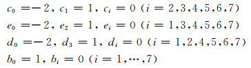
|
差分格式(4)即转化为经典的7点格式.
令
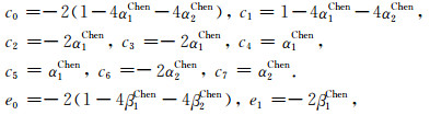
|

|
其中,满足cChen+6dChen+12eChen+8fChen=1.差分格式(4)即转化为ADM 27点格式(Chen 2014).
致谢谨此祝贺姚振兴先生从事地球物理教学科研工作60周年.
Brossier R, Operto S, Virieux J.
2009. Seismic imaging of complex onshore structures by 2D elastic frequency-domain full-waveform inversion. Geophysics, 74(6): WCC105-WCC118.
DOI:10.1190/1.3215771 |
|
Cao S H, Chen J B.
2012. A 17-point scheme and its numerical implementation for high-accuracy modeling of frequency-domain acoustic equation. Chinese Journal of Geophysics (in Chinese), 55(10): 3440-3449.
DOI:10.6038/j.issn.0001-5733.2012.10.027 |
|
Chen J B.
2012. An average-derivative optimal scheme for frequency-domain scalar wave equation. Geophysics, 77(6): T201-T210.
DOI:10.1190/geo2011-0389.1 |
|
Chen J B.
2014. A 27-point scheme for a 3D frequency-domain scalar wave equation based on an average-derivative method. Geophysical Prospecting, 62(2): 258-277.
DOI:10.1111/1365-2478.12090 |
|
Chen J B, Cao J.
2016. Modeling of frequency-domain elastic-wave equation with an average-derivative optimal method. Geophysics, 81(6): T339-T356.
DOI:10.1190/geo2016-0041.1 |
|
Chu C L, Stoffa P L.
2012. Determination of finite-difference weights using scaled binomial windows. Geophysics, 77(3): W17-W26.
DOI:10.1190/geo2011-0336.1 |
|
Fan N, Zhao L F, Xie X B, et al.
2017. A general optimal method for a 2D frequency-domain finite-difference solution of scalar wave equation. Geophysics, 82(3): T121-T132.
DOI:10.1190/geo2016-0457.1 |
|
Gu B L, Liang G H, Li Z Y.
2013. A 21-point finite difference scheme for 2D frequency-domain elastic wave modelling. Exploration Geophysics, 44(3): 156-166.
DOI:10.1071/EG12064 |
|
Holberg O.
1987. Computational aspects of the choice of operator and sampling interval for numerical differentiation in large-scale simulation of wave phenomena. Geophysical Prospecting, 35(6): 629-655.
DOI:10.1111/j.1365-2478.1987.tb00841.x |
|
Hustedt B, Operto S, Virieux J.
2004. Mixed-grid and staggered-grid finite-difference methods for frequency-domain acoustic wave modelling. Geophysical Journal International, 157(3): 1269-1296.
DOI:10.1111/j.1365-246X.2004.02289.x |
|
Jo C H, Shin C, Suh J H.
1996. An optimal 9-point, finite-difference, frequency-space, 2-D scalar wave extrapolator. Geophysics, 61(2): 529-537.
DOI:10.1190/1.1443979 |
|
Kim Y, Min D J, Shin C.
2011. Frequency-domain reverse-time migration with source estimation. Geophysics, 76(2): S41-S49.
DOI:10.1190/1.3534831 |
|
Liu L, Liu H, Liu H W.
2013. Optimal 15-point finite difference forward modeling in frequency-space domain. Chinese Journal of Geophysics (in Chinese), 56(2): 644-652.
DOI:10.6038/cjg20130228 |
|
Liu Y, Sen M K.
2009. A new time-space domain high-order finite-difference method for the acoustic wave equation. Journal of Computational Physics, 228(23): 8779-8806.
DOI:10.1016/j.jcp.2009.08.027 |
|
Loewenthal D, Mufti I R.
1983. Reversed time migration in spatial frequency domain. Geophysics, 48(5): 627-635.
DOI:10.1190/1.1441493 |
|
Min D J, Shin C, Kwon B D, et al.
2000. Improved frequency-domain elastic wave modeling using weighted-averaging difference operators. Geophysics, 65(3): 884-895.
DOI:10.1190/1.1444785 |
|
Operto S, Virieux J, Amestoy P, et al.
2007. 3D finite-difference frequency-domain modeling of visco-acoustic wave propagation using a massively parallel direct solver:A feasibility study. Geophysics, 72(5): SM195-SM211.
DOI:10.1190/1.2759835 |
|
Operto S, Virieux J, Ribodetti A, et al.
2009. Finite-difference frequency-domain modeling of viscoacoustic wave propagation in 2D tilted transversely isotropic (TTI) media. Geophysics, 74(5): T75-T95.
DOI:10.1190/1.3157243 |
|
Operto S, Brossier R, Combe L, et al.
2014. Computationally efficient three-dimensional acoustic finite-difference frequency-domain seismic modeling in vertical transversely isotropic media with sparse direct solver. Geophysics, 79(5): T257-T275.
DOI:10.1190/geo2013-0478.1 |
|
Plessix R E, Mulder W A.
2004. Frequency-domain finite-difference amplitude-preserving migration. Geophysical Journal International, 157(3): 975-987.
DOI:10.1111/j.1365-246X.2004.02282.x |
|
Pratt R G, Worthington M H.
1990. Inverse theory applied to multi-source cross-hole tomography. Part 1:Acoustic wave-equation method. Geophysical Prospecting, 38(3): 287-310.
DOI:10.1111/j.1365-2478.1990.tb01846.x |
|
Pratt R G.
1999. Seismic waveform inversion in the frequency domain, Part 1:Theory and verification in a physical scale model. Geophysics, 64(3): 888-901.
DOI:10.1190/1.1444597 |
|
Shin C, Sohn H.
1998. A frequency-space 2-D scalar wave extrapolator using extended 25-point finite-difference operator. Geophysics, 63(2): 289-296.
DOI:10.1190/1.1444323 |
|
Štekl I, Pratt R G.
1998. Accurate viscoelastic modeling by frequency-domain finite differences using rotated operators. Geophysics, 63(5): 1779-1794.
DOI:10.1190/1.1444472 |
|
Tang X D, Liu H, Zhang H, et al.
2015. An adaptable 17-point scheme for high-accuracy frequency-domain acoustic wave modeling in 2D constant density media. Geophysics, 80(6): T211-T221.
DOI:10.1190/geo2014-0124.1 |
|
Zhang H, Liu H, Liu L, et al.
2014. Frequency domain acoustic equation high-order modeling based on an average-derivative method. Chinese Journal of Geophysics (in Chinese), 57(5): 1599-1611.
DOI:10.6038/cjg20140523 |
|
Zhang J H, Yao Z X.
2012. Optimized finite-difference operator for broadband seismic wave modeling. Geophysics, 78(1): A13-A18.
DOI:10.1190/geo2012-0277.1 |
|
Zhang J H, Yao Z X.
2013. Optimized explicit finite-difference schemes for spatial derivatives using maximum norm. Journal of Computational Physics, 250: 511-526.
DOI:10.1016/j.jcp.2013.04.029 |
|
曹书红, 陈景波.
2012. 声波方程频率域高精度正演的17点格式及数值实现. 地球物理学报, 55(10): 3440–3449.
DOI:10.6038/j.issn.0001-5733.2012.10.027 |
|
刘璐, 刘洪, 刘红伟.
2013. 优化15点频率-空间域有限差分正演模拟. 地球物理学报, 56(2): 644–652.
DOI:10.6038/cjg20130228 |
|
张衡, 刘洪, 刘璐, 等.
2014. 基于平均导数方法的声波方程频率域高阶正演. 地球物理学报, 57(5): 1599–1611.
DOI:10.6038/cjg20140523 |
|