 2017, Vol. 60


2. 中国矿业大学 煤炭资源与安全开采国家重点实验室, 江苏徐州 221116
2. State Key Laboratory of Coal Resources and Safe Mining, China University of Mining and Technology, Jiangsu Xuzhou 221116, China
浅层地震勘探与直流电阻率法是解决浅地表工程地质问题最常用的地球物理勘探方法.地震走时成像在气田(Korenaga et al., 1997)、油藏(瞿辰等, 2010)、二氧化碳存储(Morency et al., 2011; Zhang et al., 2012; Carcione et al., 2012)、岩溶勘察(段成龙等, 2013; Pepe et al., 2015)、含水层结构探测(Ehosioke and Fechner, 2014)、孤石探测(郭云峰等, 2015)、矿产资源勘探(Menu et al., 2015)等领域得到较多的应用.电阻率成像技术在隧道超前预报(李术才等, 2014)、孤石探测(王俊超等, 2012; 李术才等, 2015)、岩溶勘察(张文俊等, 2014)、岩体完整性评价(Bellmunt et al., 2012; 曹权等, 2013)、大坝渗漏探测(Greve et al., 2012)、障碍物探测(Leontarakis and Apostolopoulos, 2013)、二氧化碳地下储存监测(Schmidt-Hattenberger et al., 2014)等领域也有广泛的应用.
采用地震走时法或电阻率法进行单独成像,因观测覆盖角度、数据采样率、人文干扰、成像算法中存在问题导致单一地球物理方法存在多解性,无法对地下结构进行精确成像(胡祥云等, 2006).例如,地震走时数据对高速异常体敏感,因而对其成像效果较好,一般用于解决存在速度异常的构造问题;直流电阻率数据对低阻异常体敏感,因而对低阻体具有较好的分辨能力,一般用于解决地层的富水性问题.然而这两种方法均存在较为明显的缺点,即地震走时成像对低速异常体、电阻率成像对高阻异常体存在成像阴影问题.
为了解决单一反演方法存在的多解性问题,很多学者对多数据联合反演地下介质多属性的方法进行了较为深入的研究.Lines (1988)采用岩石物理属性之间的关系建立两种勘探方法数据之间的联合反演,Haber和Oldenburg (1997)采用两种物理模型之间的结构相似性联合反演,Bosch (1999)运用两种属性之间的统计学关系进行联合反演,这三种联合反演方式可归纳为两类:(1) 建立两种或多种模型之间属性关系的联合反演;(2) 采用两种模型的结构相似作为约束条件的联合反演.当属性之间的对应关系较为复杂或没有对应关系、关系较弱时,采用结构相似进行约束的联合反演更为合理(Haber and Oldenburg, 1997; Gallardo and Meju, 2004).Gallardo和Meju (2004)首次提出以模型之间交叉梯度为结构一致约束方式的二维直流电阻率与地震折射数据的联合反演,极大促进了基于交叉梯度结构相似约束联合反演方法的发展(Gallardo and Meju, 2004; Gallardo, 2007; Fregoso and Gallardo, 2009; Moorkamp et al., 2011; 彭淼, 2012; 周丽芬, 2012; Rovetta et al., 2013; Ogunbo and Zhang, 2014; Sánchez and Delgado, 2015; Bennington et al., 2015; 李兆祥等, 2015; Wang et al., 2015; 高级和张海江, 2016).
因不同物性模型参数及灵敏度矩阵元素的数值变化范围大,可能存在量级上的巨大差异,给联合反演中求解大型灵敏度矩阵造成极大困难.Bennington等(2015)采用对基于交叉梯度约束建立的大型联合反演系统正则化的方法,实现了三维天然地震和二维大地电磁的联合反演,一定程度解决了联合反演中大型矩阵求解不稳定性问题,但在实现过程中需要显式计算地震走时与大地电磁的灵敏度矩阵,需要较大的存储空间并对单独反演程序进行修改,造成该方法实现较为困难.Um等(2014)提出了分别进行数据拟合和交叉梯度结构约束的联合反演流程,通过交替迭代进行数据约束和交叉梯度结构约束实现联合反演.虽然该流程降低了实现联合反演的难度,但是由于数据拟合与结构约束完全分开,因此迭代交替反演时较难平衡数据拟合和结构约束的权重.
针对联合反演矩阵存储空间巨大、求解不稳定及难以实现的问题,本文提出一种新的基于模型更新量及交叉梯度结构约束结合的联合反演流程,通过把单独反演得到的模型更新量加入到交叉梯度控制的结构约束之中,解决了Um等(2014)把数据拟合和交叉梯度结构约束分开反演权重难以选择的问题,同时实现数据拟合与结构约束的平衡.在具体实现过程中,把交叉梯度约束从联合反演大矩阵中分离,解决了Bennington等(2015)需要较大存储空间的问题,而且无需大幅度修改单一方法数据反演程序,为多方法数据联合反演地下介质的多属性提供了一个新的思路.
在实现基于模型更新量与交叉梯度约束的联合反演算法的基础上,本文采用了三维跨孔地震走时与直流电阻率数据,测试了反演流程的稳定性,验证了新的反演策略的有效性.相比于单独反演结果,联合反演结果减少了地震走时成像的假异常,提高了直流电阻率成像的分辨率.另外,在单独反演中可以根据L曲线等选择最优反演参数,而联合反演只需要考虑结构约束与数据拟合程度的权重大小,有效降低了联合反演权重选择的困难.
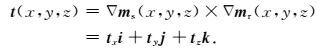
2 交叉梯度结构约束方法对于三维速度模型ms和电阻率模型mr,二者之间的交叉梯度定义为速度梯度和电阻率梯度的叉积:
|
(1) |
在三维模型情况下,垂直于Y-Z、X-Z、X-Y平面即平行于X、Y、Z方向上的交叉梯度分量分别为tx、ty、tz.其展开形式分别为:

|
在二维模型情况下,因模型沿Y方向变化为0,模型之间沿X与Z方向变化的交叉梯度只存在Y方向分量:

|
(2) |
图 1显示了三维速度与电阻率模型交叉梯度性质,速度与电阻率模型大小均为64 m×48 m×32 m.图 1a为速度模型,该模型为均匀背景中包含一个高速与一个低速异常,背景速度为2 km·s-1,高低速异常体的速度分别为3 km·s-1和1 km·s-1,大小为10 m×10 m×10 m.因异常体与背景速度具有差异性,所以其周围均具有梯度值,梯度如图中箭头方向所示.图 1b为电阻率模型,电阻率数值分布范围为100 Ωm至260 Ωm,电阻率数值只沿Z方向变化,电阻率变化规律为从Z=0 m的100 Ωm至Z=32 m的260 Ωm,变化梯度为5 Ωm·m-1.由于电阻率只在垂向上(Z)变化,所以电阻率模型的梯度只在Z方向上有非零值.速度模型与电阻率模型之间的交叉梯度如图 1c所示,从该图可以看出交叉梯度仅在X与Y方向上有值,即两个模型梯度方向相同或相反时交叉梯度值为零,反之不为零.该性质为利用交叉梯度约束反演奠定了基础,即在反演时要求速度与电阻率模型交叉梯度值趋于零,模型之间具有一致的结构.

|
图 1 两个模型交叉梯度的测试 (a)速度模型及其梯度; (b)电阻率模型及其梯度; (c)速度模型与电阻率模型的交叉梯度. Fig. 1 Tests of cross gradient on two models (a) Velocity model and its gradient; (b) Resistivity model and its gradient; (c) Cross gradient between velocity model and resistivity model. |
联合反演方法主要包括建立反演目标函数、选择反演迭代方法、联合反演具体流程、迭代终止条件等,下面对这几部分分别予以阐述.
3.1 单独反演目标函数的建立地震走时成像目标函数定义为(Aster et al., 2011):

|
(3) |
式中:f (ms)为根据地震速度模型ms计算的理论地震走时数据,ds为观测走时数据,L为速度模型平滑因子,α为速度模型平滑权重,I为单位矩阵,β为模型阻尼权重.目标函数中采用L曲线调整权重因子α、β的大小从而达到数据拟合与模型平滑之间的平衡.在实现地震走时成像时,我们采用基于射线理论的层析成像方法.首先对模型区域网格进行剖分(Sambridge, 1990),采用有限差分法求解程函方程(Vidale, 1988; Vidale, 1990)和MSFM (Multi-Stencils Fast Marching Methods)方法计算走时场(Osher and Fedkiw, 2006).为了提高反演结果的稳定性,采用二阶范数的吉洪诺夫正则化(Tikhonov and Arsenin, 1977)约束(Calvetti, 2000),并采用阻尼最小二乘LSQR法迭代求解(Paige and Saunders, 1982).
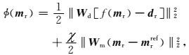
电阻率成像目标函数φ(m)可分为两个部分,即数据拟合和模型正则化,
|
(4) |
式中:f (mr)为根据电阻率模型mr计算的理论电位数据,dr为观测电位数据,为参考模型权重,mrref为电阻率参考模型,Wd为观测数据权系数矩阵、Wm为参考模型权系数矩阵,为数据拟合和参考模型之间的平衡权重因子.(4) 式中第二项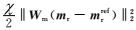
对于交叉梯度函数t (ms, mr),利用一阶泰勒展开的方法进行线性化,可写成矩阵形式为:

|
(5) |
式中

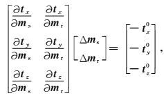
对于速度和电阻率模型,可以对二者进行改变使两个模型之间的交叉梯度为零,即最小化交叉梯度值,这样两个模型的结构就变得一致.在公式(5) 中,如果模型之间的交叉梯度t (ms, mr)为零,针对不同的交叉梯度分量可以写成下面的矩阵形式:
|
(6) |
式中Δms、Δmr分别为速度与电阻率模型更新量, 

基于交叉梯度结构约束的联合反演系统,是通过把对应于数据拟合的单个反演系统和对应于结构约束的单个反演系统(公式(6))结合而建立起来的(Gallardo and Meju, 2004).但是因为不同数据所对应的灵敏度矩阵可能存在量级上的差异,而且不同数据的反演程序相差很大,因此很难把不同数据的反演系统以及交叉梯度反演系统融合起来实现联合反演.为了解决这个问题,Um等(2014)提出了一种新的联合反演策略,即首先基于不同数据的单独反演系统对模型进行更新对数据进行拟合,然后利用交叉梯度结构约束反演系统进一步更新模型使得两个模型的结构一致.这两个步骤交替进行直至数据拟合和交叉梯度最小化.这种联合反演方式把结构约束与数据拟合分开交替地进行,虽然可以直接利用现有的反演系统进行联合反演,但是在该流程实际实现的过程当中,很难平衡数据的拟合和结构一致的约束.为了解决这个问题,高级和张海江(2016)提出了一种新的基于交叉梯度交替结构约束的联合反演流程,即在进行地震走时反演时,用电阻率模型同时约束速度模型的结构,在直流电阻率反演时,同时用速度结构约束电阻率结构,这两个步骤交替进行直至收敛.这种交替结构约束的联合反演策略很容易实现结构约束和数据拟合之间的平衡.该反演策略要求把单独反演系统的灵敏度矩阵提取出来,和交叉梯度约束对应的灵敏度矩阵组合在一起,但是在某些情况下如三维直流电阻率反演很难显式提取出灵敏度矩阵.
所以为了解决上面的问题,基于Um等(2014)的联合反演策略,我们提出一种新的联合反演策略来实现数据拟合和结构一致性的平衡.把单独地震走时反演与直流电阻率反演得到的速度更新量Δms0与电阻率更新量Δmr0与只基于交叉梯度结构约束的反演系统(6) 结合起来,即把Δms0、Δmr0加入到基于交叉梯度的反演系统中,用于约束基于交叉梯度最小化的线性反演系统,得到新的速度更新量Δms和新的电阻率更新量Δmr,实现数据拟合和结构一致性的平衡.在三维模型情况下,新的联合反演系统可以写成式(7):
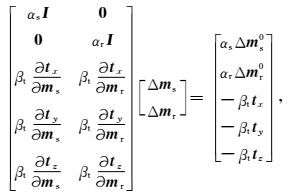
|
(7) |
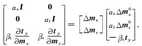
式中:αs为速度更新量权重,αr为电阻率更新量权重,βt为结构一致性约束权重.在二维模型情况下,式(7) 可以简化为式(8) 的形式:

|
(8) |
在公式(7) 和(8) 中,通过调整αs,αr和βt三个参数的相对大小,就可以达到数据拟合和结构一致约束之间的平衡.
3.3 联合反演流程图 2为本文提出的基于模型更新量及交叉梯度

|
图 2 三维地震走时和直流电阻率联合反演流程图 Fig. 2 Flow chart of proposed scheme for 3D seismic travel time and DC resistivity joint inversion |
结构约束的地震走时和电阻率联合反演流程图,包括以下几个主要步骤:
(1) 输入初始速度模型与电阻率模型,并计算二者之间的交叉梯度;
(2) 根据公式(3) 和(4) 定义的目标函数分别进行地震走时和电阻率单独成像,求解出速度模型更新量与电阻率模型更新量;
(3) 根据交叉梯度结构约束、速度和电阻率模型更新量,基于公式(7) 或者(8) 所表示的联合反演矩阵,求解得到新的速度模型与电阻率模型更新量;
(4) 更新速度与电阻率模型,并计算更新后的速度模型与电阻率模型之间的交叉梯度以及地震走时数据和电位数据的残差;
(5) 判断数据拟合和交叉梯度值是否满足迭代终止条件,若满足直接输出结果,若不满足返回步骤(2).
通常采用的迭代终止条件包括:迭代次数、每次迭代残差下降的梯度、残差剩余量占初始残差百分比、模型更新量大小等.本文采用的迭代终止即假设迭代过程已经收敛的条件为电阻率或地震走时残差下降量低于某一百分比时迭代终止(例如迭代残差下降量小于1%).
由于不同反演方法得到的模型更新量数量级具有较大差异,因此在联合反演中,不同方法之间模型更新量的权重选择极为重要.地震走时成像中参与计算的模型参数为慢度,其数量级为10-3,模型更新量数据数量级为10-4;电阻率成像中参与计算的参数为电导率的自然对数,其数量级为101,更新量数据量级为100.基于两种模型更新量数量级的差异,在设置地震慢速与电阻率模型更新量之间平衡的权重参数时,需要使αs比αr高4个数量级.本文设置的权重参数αs为100,αr为10-4,这样就改善了地震走时与电阻率数据联合反演时两种参数的数量级及变化范围不同的问题,为联合反演权重选择提供了参考依据.βt从10-10至1010以间隔10倍关系分别计算地震走时、电阻率观测数据拟合残差与交叉梯度值,根据L曲线选择合适的结构约束权重βt(Aster et al., 2011).本文对于前5次迭代将βt设置为102,第6次至第20次迭代将βt设置为103.
综合起来,两种不同成像方法的联合反演参数选择分为两步:
(1) 首先根据两种模型参数的更新量数量级,确定两种模型之间合适的权重参数使两种模型均起到结构约束的作用.
(2) 根据L曲线等权重选择方法确定结构约束与数据拟合之间的平衡.
4 合成数据测试为了验证本文提出的基于模型更新量的联合反演流程,我们利用三维跨孔地震走时与三维跨孔直流电阻率联合反演进行数值试验.由于本文提出的联合反演方法不需要修改单个反演程序,因此,可以非常便捷地实现两者的联合反演.
图 3为地震走时与直流电阻率跨孔观测装置布置示意图.在该算例中,我们设计了符合实际工程施工条件的4个钻孔式的跨孔观测装置.假设模型地表一个角为(0, 0) 点,则4个钻孔的坐标分别为:Bore1(3, 3)、Bore2(14, 3)、Bore3(14, 16)、Bore4(3, 16),坐标的单位为m,孔深均为12 m.

|
图 3 三维跨孔地震走时与直流电阻率观测装置 (a)地震观测装置,小四方块表示地震传感器的分布,井(黑线)中布设的震源以圆圈表示;(b)直流电阻率观测装置,小四方块表示电极的分布. Fig. 3 Observation geometry for cross-hole seismic travel time and DC resistivity surveys (a) Seismic survey apparatus. Squares represent geophones. Circles represent seismic sources. Black lines indicate locations of wells. (b) DC resistivity survey apparatus. Squares represent electrodes. |
在地震走时跨孔装置中,每个孔中设置11个激发点、11个接收点,激发点和接收点间距均为1 m;地表布设56个接收点,间距为1 m×1 m.数据采集时,每个孔中的激发对应的接收点为除去激发点所在钻孔之外的所有接收点.
在电阻率跨孔装置中,每个孔中放置10个电极,电极距为1 m;地表布设56个电极,间距为1 m×1 m.数据采集时,地表和孔中所有的电极任取两个作为供电电极,其余电极全部采集观测电位.
我们首先通过均匀速度模型2000 m·s-1和均匀电阻率模型100 Ωm来验证三维地震走时场与三维电位场的数值计算精度.比较数值计算结果与解析结果发现,两者误差均达到0.01%的误差水平.由于实际反演迭代终止条件一般选择数据拟合为1%的拟合水平,因此,本文采用的地震走时与直流电阻率正演算法能够满足反演精度要求.图 4为均匀背景中存在一个高速异常体的理论速度模型与对应的三维地震走时场,其中背景速度为2000 m·s-1,高速异常体速度为3000 m·s-1,异常体大小为3 m×3 m×2 m;图 5为均匀背景电阻率中存在一个高阻异常体的理论电阻率模型与对应的三维电位场,其中背景电阻率为100 Ωm,高阻体电阻率为1000 Ωm,异常体大小为3 m×3 m×2 m.
基于图 4、图 5中所示的理论速度模型和理论电阻率模型,通过正演计算得到了理论地震走时和电位数据,然后均加入了3%的高斯噪声构建了用于模型测试的数据.地震走时和电阻率成像所用的初始速度模型和初始电阻率模型均为均匀模型,初始速度为2000 m·s-1,初始电阻率为100 Ωm.单独地震走时、单独电阻率成像以及联合反演得到的速度模型和电阻率模型的三维立体图、等深度切片及沿Y方向的侧向切片分别显示在图 6、图 7和图 8.从图中可以看出,地震走时成像与电阻率成像均能较好地分辨出异常的水平中心位置及形态;但在垂向上,地震走时成像具有较高的分辨率,而电阻率成像得到的异常体向地表延伸,无法较好地刻画异常体的纵向形态.相比较来说,通过联合反演提高了电阻率成像对异常体的纵向分辨率,同时由于电阻率成像产生干扰异常较少,可以通过交叉梯度的约束减少地震走时成像的拖尾异常.

|
图 4 速度模型与三维走时场 (a)速度模型, 高速异常大小为3 m×3 m×2 m, 距离地面3m; (b)对应的三维走时场等位面. Fig. 4 Velocity model and corresponding 3D travel time field (a) Velocity model with a high velocity anomaly of 3 m×3 m×2 m and 3 m below the ground surface; (b) 3D travel time isosurface shown as the curved face. |

|
图 5 电阻率模型与对应的三维电位场 (a)电阻率模型, 高阻异常大小为3 m×3 m×2m, 距离地面3m; (b)在两个电极供电情况下的电位场等位面. Fig. 5 Resistivity model and the corresponding 3D electrical field (a) Resistivity model with a high resistivity anomaly of 3 m×3 m×2 m and 3 m below the ground surface; (b) 3D electrical field with potential isosurface shown as the curved face. |

|
图 6 单独反演和联合反演得出的速度和电阻率的三维立体图 (a)真实速度模型;(b)单独反演速度结果;(c)联合反演速度结果;(d)电阻率模型;(e)单独反演电阻率结果;(f)联合反演电阻率结果. Fig. 6 3D view of seismic velocity and electrical resistivity models from separate and joint inversions (a) True velocity model; (b) Velocity model from separate inversion; (c) Velocity model from joint inversion; (d) Real resistivity model; (e) Resistivity model from separate inversion; (f) Resistivity model from joint inversion. |

|
图 7 单独反演和联合反演得出的速度和电阻率等深度切片图(Z=5 m) (a)真实速度模型;(b)单独反演速度模型;(c)联合反演速度模型;(d)真实电阻率模型;(e)单独反演电阻率模型;(f)联合反演电阻率模型. Fig. 7 Slices of seismic velocity and electrical resistivity models at Z=5 m from separate and joint inversions (a) True velocity model; (b) Velocity model from separate inversion; (c) Velocity model from joint inversion; (d) Resistivity model; (e) Resistivity model from separate inversion; (f) Resistivity model from joint inversion. |

|
图 8 单独反演和联合反演得出的速度和电阻率剖面图(Y=10 m) (a)真实速度模型;(b)单独反演速度模型;(c)联合反演速度模型;(d)真实电阻率模型;(e)单独反演电阻率模型;(f)联合反演电阻率模型. Fig. 8 Cross sections of seismic velocity and electrical resistivity models at Y=10 m from separate and joint inversions (a) True velocity model; (b) Velocity model from separate inversion; (c) Velocity model from joint inversion; (d) True resistivity model; (e) Resistivity model from separate inversion; (f) Resistivity model from joint inversion. |
图 7和图 8显示的联合反演结果表明联合反演比单独反演具有较大的优势.在该测试中,两个模型中对应的异常为正比例关系,即高速对应高阻.为了进一步研究基于交叉梯度结构约束联合反演的适用范围,本文设计了异常结构属性呈反比例对应关系的速度和电阻率模型,其中速度模型与图 4中速度模型一致,而电阻率模型为在均匀背景电阻率(100 Ωm)中存在一个低阻异常体,低阻异常体的电阻率值为10 Ωm,大小为3 m×3 m×2 m.图 9和图 10为反比例模型对应的单独反演和联合反演得到的速度模型和电阻率模型在深度上的切片和沿Y方向的侧向切片.从图中可以看出,与正比例异常模型一样,联合反演对于反比例异常模型也能得到较好的反演结果.

|
图 9 单独反演和联合反演得出的速度和电阻率等深度切片图(Z=5 m) (a)真实速度模型;(b)单独反演速度模型;(c)联合反演速度模型;(d)真实电阻率模型;(e)单独反演电阻率模型;(f)联合反演电阻率模型. Fig. 9 Slices of seismic velocity and electrical resistivity models at Z=5 m from separate and joint inversions (a) True velocity model; (b) Velocity model from separate inversion; (c) Velocity model from joint inversion; (d) True resistivity model; (e) Resistivity model from separate inversion; (f) Resistivity model from joint inversion. |

|
图 10 单独反演和联合反演得出的速度和电阻率剖面图(Y=10 m) (a)真实速度模型;(b)单独反演速度模型;(c)联合反演速度模型;(d)真实电阻率模型;(e)单独反演电阻率模型;(f)联合反演电阻率模型. Fig. 10 Cross sections of seismic velocity and electrical resistivity models at Y=10 m from separate and joint inversions (a) True velocity model; (b) Velocity model from separate inversion; (c) Velocity model from joint inversion; (d) True resistivity model; (e) Resistivity model from separate inversion; (f) Resistivity model from joint inversion. |
在实际地质工程勘探时,若勘探区内有钻孔时,在钻孔中测井或取样可以测得垂向岩层的速度和电阻率值.通过孔中已知的速度和电阻率值,可以构建一维层状参考速度和电阻率模型.在进行联合反演时,可以利用钻孔中已知的垂向上的界面信息来约束三维速度和电阻率模型的反演.式(7) 中阻尼权重系数αs和αr分别替换为diag(∂mspriori/∂z)和diag(∂mrpriori/∂z)得到式(9),其中ms、mr分别为上一次迭代得到的速度模型和电阻率模型.mspriori和mrpriori分别根据已知速度和电阻率建立的层状参考速度和电阻率模型,∂mspriori/∂z和∂mrpriori/∂z分别为先验速度模型和电阻率模型在垂向上的梯度,因为先验模型为层状模型,速度和电阻率只在模型垂向上变化,所以∂mspriori/∂z和∂mrpriori/∂z计算得到的垂向梯度就保留了已知参考模型的上下边界信息,然后把∂mspriori/∂z和∂mrpriori/∂z分别对角化并与单位矩阵I相乘,在通过式(9) 求解新的速度更新量Δms和电阻率更新量Δmr时,就保留了上一次反演得到的速度更新量Δms0和电阻率更新量Δmr0中的边界信息,如式(9) 所示:
|
(9) |
式中:diag(∂mspriori/∂z)为先验速度模型mspriori纵向梯度对角化,diag(∂mrpriori/∂z)为先验电阻率模型mrpriori纵向梯度对角化.
图 11和图 12分别为加入垂向层状速度与电阻率先验模型约束的三维跨孔地震走时与直流三维电阻率联合反演模型的等深度切片与侧向剖面图.该算例采用的观测装置与图 3所示的一致,在均匀速度(2000 m·s-1)、电阻率(100 Ωm)模型中设置了两个异常体,分别为高速高阻体(2500 m·s-1, 1000 Ωm)和低速低阻体(1500 m·s-1, 10 Ωm).异常体大小为3 m×3 m×3 m,距离地表 3 m.速度和电阻率反演初始模型分别为2000 m·s-1和100 Ωm.从加入先验信息的联合反演结果可以看出,相比较于地震走时数据与电位数据单独反演的结果,联合反演得到的速度与电阻率模型均具有更好的形态及更准确的异常体中心成像,与真实模型相比速度异常与电阻率异常均得到了较好的数值恢复.

|
图 11 加入先验界面信息约束的联合反演等深度切片图(Z=5 m) (a)真实速度模型;(b)单独反演速度模型;(c)联合反演速度模型;(d)真实电阻率模型;(e)单独反演电阻率模型;(f)联合反演电阻率模型. Fig. 11 Slices of seismic velocity and electrical resistivity models at Z=5 m from joint inversion with additional constraint from a priori interface information (a) True velocity model; (b) Velocity model from separate inversion; (c) Velocity model from joint inversion; (d) True resistivity model; (e) Resistivity model from separate inversion; (f) Resistivity model from joint inversion. |

|
图 12 加入先验界面信息约束的联合反演剖面图(X=8 m) (a)真实速度模型;(b)单独反演速度模型;(c)联合反演速度模型;(d)真实电阻率模型;(e)单独反演电阻率模型;(f)联合反演电阻率模型. Fig. 12 Cross sections of seismic velocity and electrical resistivity models at X=8 m from joint inversion with added constraint from a priori interface information (a) True velocity model; (b) Velocity model from separate inversion; (c) Velocity model from joint inversion; (d) True resistivity model; (e) Resistivity model from separate inversion; (f) Resistivity model from joint inversion. |
地球物理联合反演一般基于多方法之间的互相约束实现,包括基于岩石物理属性联系与结构一致两种约束方式的联合反演.本文在实现三维地震走时与直流电阻率联合反演时采用了基于交叉梯度结构约束的方法.但是传统的基于交叉梯度结构约束的联合反演可能存在如下问题:
(1) 构建联合反演矩阵时,反演系数矩阵较为庞大,需要较大的计算及存储成本.
(2) 不同地球物理方法对岩石属性灵敏度不同,造成不同方法的反演系数矩阵数量级差距较大,致使联合反演系数矩阵的求解存在不稳定性.
(3) 为了构建联合反演矩阵,需要对单一反演程序进行修改,给联合反演程序实现带来巨大困难.
针对上述联合反演存在的问题,本文提出了基于单个数据单独反演得到的模型更新量与交叉梯度结构约束相结合的联合反演策略,实现数据拟合和结构一致之间的拟合.该反演策略具有以下优势:
(1) 不需要对单个数据的反演程序进行改动,只需要给出其迭代一次的模型更新量即可,极大地简化了联合反演的实现难度.采用本文提出的新的联合反演流程,可以方便地实现多属性联合反演.例如实现直流电测深与多道面波的联合反演,可提高直流电测深的纵向分辨率及多道面波的横向分辨率.
(2) 在单个数据反演中可以有效地选择数据拟合权重与模型平滑权重,而在联合反演中只需要平衡结构约束与数据拟合即可,解决了传统的联合反演系统中权重难以选择的问题(Bennington et al., 2015; Zhou et al., 2015).
(3) 与Um等(2014)的反演策略相比较,本文提出的联合反演策略可以很容易地实现结构一致和数据拟合之间的平衡.
通过三维跨孔地震走时与直流电阻率联合反演对本文提出的联合反演流程进行了测试,结果证明了该联合反演策略的正确性与有效性.通过电阻率结构约束有效减少了速度反演结果中的拖尾等干扰异常,通过速度结构的约束有效提高了电阻率反演结果的分辨率,进而总体提高了地震走时与电阻率的成像效果.
致谢感谢评审专家对论文提出的宝贵修改意见.
| Aster R C, Borchers B, Thurber C H. 2011. Parameter Estimation and Inverse Problems. Boston: Academic Press. | |
| Bellmunt F, Marcuello A, Ledo J, et al. 2012. Time-lapse cross-hole electrical resistivity tomography monitoring effects of an urban tunnel. Journal of Applied Geophysics, 87: 60-70. DOI:10.1016/j.jappgeo.2012.09.003 | |
| Bennington N L, Zhang H J, Thurber C H, et al. 2015. Joint inversion of seismic and magnetotelluric data in the Parkfield region of California using the normalized cross-gradient constraint. Pure and Applied Geophysics, 172(5): 1033-1052. DOI:10.1007/s00024-014-1002-9 | |
| Bosch M. 1999. Lithologic tomography:From plural geophysical data to lithology estimation. Journal of Geophysical Research:Solid Earth, 104(B1): 749-766. DOI:10.1029/1998JB900014 | |
| Calvetti D, Morigi S, Reichel L, et al. 2000. Tikhonov regularization and the L-curve for large discrete ill-posed problems. Journal of Computational and Applied Mathematics, 123(1-2): 423-446. DOI:10.1016/S0377-0427(00)00414-3 | |
| Cao Q, Xiang W, Jia H L, et al. 2013. Application of cross-hole ultra-density resistivity method to detection of spherically weathered granite. Journal of Engineering Geology, 21(5): 730-735. | |
| Carcione J M, Gei D, Picotti S, et al. 2012. Cross-hole electromagnetic and seismic modeling for CO2 detection and monitoring in a saline aquifer. Journal of Petroleum Science and Engineering, 100: 162-172. DOI:10.1016/j.petrol.2012.03.018 | |
| Duan C L, Yan C H, Xu B T, et al. 2013. The application of cross-hole seismic CT method in the karst cave exploration of metro engineering construction. Geological Review, 59(6): 1242-1248. | |
| Ehosioke S I, Fechner T. 2014. Application of cross-hole seismic tomography in characterization of heterogeneous aquifers.//Near Surface Geoscience 2014-20th European Meeting of Environmental and Engineering Geophysics. EAGE. Extended Abstract, doi:10.3997/2214-4609.20142018. | |
| Fregoso E, Gallardo L A. 2009. Cross-gradients joint 3D inversion with applications to gravity and magnetic data. Geophysics, 74(4): L31-L42. DOI:10.1190/1.3119263 | |
| Gallardo L A, Meju M A. 2004. Joint two-dimensional DC resistivity and seismic travel time inversion with cross-gradients constraints. Journal of Geophysical Research:Solid Earth, 109(B3): B03311. DOI:10.1029/2003JB002716 | |
| Gallardo L A. 2007. Multiple cross-gradient joint inversion for geospectral imaging. Geophysical Research Letters, 34(19): L19301. DOI:10.1029/2007GL030409 | |
| Gao J, Zhang H J. 2016. Two-dimensional joint inversion of seismic velocity and electrical resistivity using seismic travel times and full channel electrical measurements based on alternating cross-gradient structural constraint. Chinese Journal of Geophysics, 59(11): 4310-4322. DOI:10.6038/cjg20161131 | |
| Greve A K, Acworth R I, Kelly B F J. 2012. 3D Cross-hole resistivity tomography to monitor water percolation during irrigation on cracking soil. Soil Research, 49(8): 661-669. | |
| Guo Y F, Hu X J, You J M. 2015. The exploitation of straight and curve tracing method in boulders prospected by seismic cross-hole tomography. Chinese Journal of Engineering Geophysics, 12(3): 361-366. | |
| Haber E, Oldenburg D. 1997. Joint inversion:a structural approach. Inverse Problems, 13(1): 63-77. DOI:10.1088/0266-5611/13/1/006 | |
| Hu X Y, Yang D K, Liu S H, et al. 2006. The developing trends of environmental and engineering geophysics. Progress in Geophysics, 21(2): 598-604. DOI:10.3969/j.issn.1004-2903.2006.02.041 | |
| Korenaga J, Holbrook W S, Singh S C, et al. 1997. Natural gas hydrates on the southeast US margin:Constraints from full waveform and travel time inversions of wide-angle seismic data. Journal of Geophysical Research-All Series, 102(B7): 15345-15365. DOI:10.1029/97JB00725 | |
| Leontarakis K, Apostolopoulos G V. 2013. Model Stacking (MOST) technique applied in cross-hole ERT field data for the detection of Thessaloniki ancient walls' depth. Journal of Applied Geophysics, 93: 101-113. DOI:10.1016/j.jappgeo.2013.04.004 | |
| Li S C, Su M X, Xue Y G, et al. 2014. Study on computed tomography of cross-hole resistivity in urban subway geological prediction. Chinese Journal of Rock Mechanics and Engineering, 33(5): 913-920. | |
| Li X C, Liu Z Y, Liu B, et al. 2015. Boulder detection method for metro shield zones based on ross-hole resistivity tomography and its physical model tests. Chinese Journal of Geotechnical Engineering, 37(3): 446-457. | |
| Li Z X, Tan H D, Fu S S, et al. 2015. Two-dimensional synchronous inversion of TDIP with cross-gradient constraint. Chinese Journal of Geophysics, 58(12): 4718-4726. DOI:10.6038/cjg20151232 | |
| Lines L R, Schultz A K, Treitel S. 1988. Cooperative inversion of geophysical data. Geophysics, 53(1): 8-20. DOI:10.1190/1.1442403 | |
| McGillivray P R, Oldenburg D W. 1990. Methods for calculating Fréchet derivatives and sensitivities for the non-linear inverse problem:a comparative study. Geophysical Prospecting, 38(5): 499-524. DOI:10.1111/gpr.1990.38.issue-5 | |
| Menu F, Kepic A, Greenwood A. 2015. Crosshole seismic reflection to delineate Rosebery type volcanogenic massive sulphide ore lens.//85th Annual Meeting. Society of Exploration Geophysicists. Expanded Abstracts. | |
| Moorkamp M, Heincke B, Jegen M, et al. 2011. A framework for 3-D joint inversion of MT, gravity and seismic refraction data. Geophysical Journal International, 184(1): 477-493. DOI:10.1111/gji.2010.184.issue-1 | |
| Morency C, Luo Y, Tromp J. 2011. Acoustic, elastic and poroelastic simulations of CO2 sequestration crosswell monitoring based on spectral-element and adjoint methods. Geophysical Journal International, 185(2): 955-966. DOI:10.1111/gji.2011.185.issue-2 | |
| Ogunbo J N, Zhang J. 2014. Joint seismic traveltime and TEM inversion for near surface imaging.//84th Annual Meeting. Society of Exploration Geophysicists. Expanded Abstracts. | |
| Osher S, Fedkiw R. 2006. Level Set Methods and Dynamic Implicit Surfaces. New York:Springer Science & Business Media. | |
| Paige C C, Saunders M A. 1982. LSQR:An algorithm for sparse linear equations and sparse least squares. ACM Transactions on Mathematical Software (TOMS), 8(1): 43-71. DOI:10.1145/355984.355989 | |
| Peng M. 2012. Joint inversion of magnetotelluric and teleseismic data[Ph. D. thesis] (in Chinese). Beijing:China University of Geosciences (Beijing). | |
| Pepe P, Martimucci V, Parise M. 2015. Geological and geophysical techniques for the identification of subterranean cavities.//Lollino G, Manconi A, Guzzetti F eds. Engineering Geology for Society and Territory. Cham:Springer International Publishing, 483-487. | |
| Pidlisecky A, Haber E, Knight R. 2007. RESINVM3D:A 3D resistivity inversion package. Geophysics, 72(2): H1-H10. DOI:10.1190/1.2402499 | |
| Qu C, Yang W C, Yu C Q. 2010. An application of high resolution P and S wave crosshole tomography in understanding the reservoir features. Chinese Journal of Geophysics, 53(12): 2944-2954. DOI:10.3969/j.issn.0001-5733.2010.12.018 | |
| Rovetta D, Colombo D, Curiel E S, et al. 2013. 3D seismic-gravity simultaneous joint inversion for near surface velocity estimation.//75th EAGE Conference & Exhibition Incorporating. SPE. | |
| Sánchez A M L, Delgado L A G. 2015. 2D cross-gradient joint inversion of magnetic and gravity data across the Capricorn Orogen in Western Australia.//85th Annual Meeting. Society of Exploration Geophysicists. Expanded Abstracts. | |
| Sambridge M S. 1990. Non-linear arrival time inversion:constraining velocity anomalies by seeking smooth models in 3-D. Geophysical Journal International, 102(3): 653-677. DOI:10.1111/gji.1990.102.issue-3 | |
| Schmidt-Hattenberger C, Bergmann P, Labitzke T, et al. 2014. CO2 Migration monitoring by means of electrical resistivity tomography (ERT)-review on five years of operation of a permanent ERT system at the Ketzin pilot site. Energy Procedia, 63: 4366-4373. DOI:10.1016/j.egypro.2014.11.471 | |
| Tikhonov A N, Arsenin V I A. 1977. Solutions of Ill-Posed Problems. New York:Winston. | |
| Um E S, Commer M, Newman G A. 2014. A strategy for coupled 3D imaging of large-scale seismic and electromagnetic data sets:Application to subsalt imaging. Geophysics, 79(3): ID1-ID13. DOI:10.1190/geo2013-0053.1 | |
| Vidale J. 1988. Finite-difference calculation of travel times. Bulletin of the Seismological Society of America, 78(6): 2062-2076. | |
| Vidale J E. 1990. Finite-difference calculation of traveltimes in three dimensions. Geophysics, 55(5): 521-526. DOI:10.1190/1.1442863 | |
| Wang H, Li Y G, Chen C. 2015. 3D joint inversion of gravity gradiometry and magnetic data in spherical coordinates with the cross-gradient constraint.//85th Annual Meeting. Society of Exploration Geophysicists. Expanded Abstracts. | |
| Wang J C, Shi X M, Wang F F, et al. 2012. The physical experiment research in laboratory of cross-hole electric resistivity tomography for detecting boulders. Computerized Tomography Theory and Application, 21(4): 647-657. | |
| Wu X P, Xu G M. 2000. Study on 3D resistivity inversion using conjugate gradient method. Chinese Journal of Geophysics, 43(3): 420-427. DOI:10.3321/j.issn:0001-5733.2000.03.016 | |
| Zhang F J, Juhlin C, Cosma C, et al. 2012. Cross-well seismic waveform tomography for monitoring CO2 injection:a case study from the Ketzin Site, Germany. Geophysical Journal International, 189(1): 629-646. DOI:10.1111/gji.2012.189.issue-1 | |
| Zhang W J, Li X C, Su M X, et al. 2014. Detection method of karst caves in city subway based on the cross-hole resistivity tomography. Journal of Shandong University (Engineering Science), 44(3): 75-82. | |
| Zhou J J, Meng X H, Guo L H, et al. 2015. Three-dimensional cross-gradient joint inversion of gravity and normalized magnetic source strength data in the presence of remanent magnetization. Journal of Applied Geophysics, 119: 51-60. DOI:10.1016/j.jappgeo.2015.05.001 | |
| Zhou L F. 2012. Two dimensional joint inversion of MT and seismic data[Master's thesis] (in Chinese). Beijing:China University of Geosciences (Beijing). | |
| 曹权, 项伟, 贾海梁, 等. 2013. 跨孔超高密度电阻率法在球状风化花岗岩体探测中的应用. 工程地质学报, 21(5): 730–735. | |
| 段成龙, 阎长虹, 许宝田, 等. 2013. 跨孔地震CT技术在地铁工程施工溶洞探测方面的应用. 地质论评, 59(6): 1242–1248. | |
| 高级, 张海江. 2016. 基于交叉梯度交替结构约束的二维地震走时与全通道直流电阻率联合反演. 地球物理学报, 59(11): 4310–4322. DOI:10.6038/cjg20161131 | |
| 郭云峰, 胡晓娟, 游敬密. 2015. 地震波跨孔CT探测孤石中直线与曲线追踪法的应用. 工程地球物理学报, 12(3): 361–366. | |
| 胡祥云, 杨迪坤, 刘少华, 等. 2006. 环境与工程地球物理的发展趋势. 地球物理学进展, 21(2): 598–604. DOI:10.3969/j.issn.1004-2903.2006.02.041 | |
| 李术才, 苏茂鑫, 薛翊国, 等. 2014. 城市地铁跨孔电阻率CT超前地质预报方法研究. 岩石力学与工程学报, 33(5): 913–920. | |
| 李术才, 刘征宇, 刘斌, 等. 2015. 基于跨孔电阻率CT的地铁盾构区间孤石探测方法及物理模型试验研究. 岩土工程学报, 37(3): 446–457. DOI:10.11779/CJGE201503008 | |
| 李兆祥, 谭捍东, 付少帅, 等. 2015. 基于交叉梯度约束的时间域激发极化法二维同步反演. 地球物理学报, 58(12): 4718–4726. DOI:10.6038/cjg20151232 | |
| 彭淼. 2012. 大地电磁与天然地震数据联合反演研究[博士论文]. 北京: 中国地质大学(北京). | |
| 瞿辰, 杨文采, 于常青. 2010. 井间高分辨率纵横波层析成像研究井间油藏. 地球物理学报, 53(12): 2944–2954. DOI:10.3969/j.issn.0001-5733.2010.12.018 | |
| 王俊超, 师学明, 万方方, 等. 2012. 探测孤石高阻体的跨孔电阻率CT水槽物理模拟实验研究. CT理论与应用研究, 21(4): 647–657. | |
| 吴小平, 徐果明. 2000. 利用共轭梯度法的电阻率三维反演研究. 地球物理学报, 43(3): 420–426. DOI:10.3321/j.issn:0001-5733.2000.03.016 | |
| 张文俊, 李术才, 苏茂鑫, 等. 2014. 基于井间电阻率成像的城市地铁溶洞探测方法. 山东大学学报(工学版), 44(3): 75–82. DOI:10.6040/j.issn.1672-3961.0.2013.343 | |
| 周丽芬. 2012. 大地电磁与地震数据二维联合反演研究[硕士论文]. 北京: 中国地质大学(北京). http://cdmd.cnki.com.cn/article/cdmd-11415-1012364756.htm | |